| Issue |
A&A
Volume 702, October 2025
|
|
|---|---|---|
| Article Number | A5 | |
| Number of page(s) | 14 | |
| Section | Planets, planetary systems, and small bodies | |
| DOI | https://doi.org/10.1051/0004-6361/202556273 | |
| Published online | 26 September 2025 | |
Monte Carlo simulations of magnetospheric ion precipitation into Triton's upper atmosphere: Sputtering, energy deposition, charge exchange, and ionization
1
Planetary Environmental and Astrobiological Research Laboratory (PEARL), School of Atmospheric Sciences, Sun Yat-sen University,
Zhuhai,
Guangdong,
PR China
2
Center for Excellence in Comparative Planetology, Chinese Academy of Sciences,
Hefei,
Anhui,
PR China
★ Corresponding author: This email address is being protected from spambots. You need JavaScript enabled to view it.
Received:
5
July
2025
Accepted:
18
August
2025
Abstract
Context. Magnetospheric ion precipitation is an important driver of energy and mass transfer in a planet’s upper atmosphere. When energetic ions penetrate an atmosphere, they undergo a cascade of interactions with background species, including elastic scattering, charge exchange, excitation, dissociation, and ionization. These processes can alter the atmospheric composition and potentially contribute to atmospheric escape, a process known as sputtering.
Aims. We investigated the effects of magnetospheric N+ and H+ precipitation on Triton’s upper atmosphere.
Methods. We established a one-dimensional test particle Monte Carlo model to simulate the process.
Results. Our simulations indicate a total nitrogen escape rate of approximately (0.2-2)× 1026 s−1, primarily resulting from incident N+ ions. This rate is comparable to the previously reported values for Jeans escape and chemical escape, indicating that ion precipitation is a substantial contributor to Triton’s atmospheric loss. We also quantified the energy deposition, charge exchange, and ionization rates along with the energy degradation of incident ions, and assessed their sensitivities to ion energy, incidence angle, and scattering angle distribution.
Conclusions. While magnetospheric electron precipitation likely dominates atmospheric ionization on Triton, our estimations suggest that the contribution of ion precipitation is non-negligible.
Key words: planets and satellites: atmospheres / planets and satellites: individual: Triton
© The Authors 2025
 Open Access article, published by EDP Sciences, under the terms of the Creative Commons Attribution License (https://creativecommons.org/licenses/by/4.0), which permits unrestricted use, distribution, and reproduction in any medium, provided the original work is properly cited.
This article is published in open access under the Subscribe to Open model. This email address is being protected from spambots. You need JavaScript enabled to view it. to support open access publication.
1 Introduction
Magnetospheric ion precipitation constitutes a critical mechanism influencing the evolution of planetary atmospheres and ionospheres. When energetic ions penetrate a planet’s upper atmosphere, they engage in a cascade of collisions with background species. These interactions facilitate the transfer of energy through multiple processes, including elastic scattering, charge exchange, excitation, dissociation, and ionization. The effect of these collisions results in significant alterations to the atmospheric energy balance and composition. This mechanism is particularly significant for celestial bodies that lack a global intrinsic magnetic field – such as Mars and Venus (e.g., Luhmann & Kozyra 1991; Fang et al. 2013; Leblanc et al. 2015), as well as for moons like Titan (e.g., Cravens et al. 2008; Snowden & Higgins 2021) – which are directly exposed to the intense plasma environment of their host planet or the solar wind. In some instances, the energy imparted to atmospheric constituents during such collisions can exceed their gravitational binding energy, enabling atmospheric particles to escape into space. This nonthermal escape process, commonly referred to as atmospheric sputtering, has been identified as a major contributor to longterm atmospheric loss and evolutionary change on unmagnetized planetary bodies (Johnson 1994; Johnson et al. 2008).
Triton, Neptune’s largest moon, possesses a tenuous and cold atmosphere primarily composed of molecular nitrogen, with minor constituents such as methane and carbon monoxide (e.g., Broadfoot et al. 1989; Krasnopolsky et al. 1992, 1993). The Voyager 2 radio occultation experiment revealed a surprisingly dense ionosphere on Triton, with peak electron densities reaching ~104 cm−3, an order of magnitude higher than those observed on Titan (Lindal et al. 1983; Tyler et al. 1989). Given that Triton is farther from the Sun than Titan, solar radiation alone is insufficient to account for such ionospheric densities. An additional ionization source, likely in the form of energetic electrons originating from Neptune’s magnetosphere, has been proposed to resolve this discrepancy (Majeed et al. 1990; Strobel et al. 1990b; Lellouch et al. 1992). Due to the significant tilt and offset of Neptune’s magnetic dipole, combined with Triton’s high-inclination retrograde orbit, the moon periodically traverses regions of increased plasma flux, especially during its passage through the magneto-tail (Ness et al. 1989; Krimigis et al. 1989). In these regions, precipitating magnetospheric ions and electrons collide with ambient neutrals in Triton’s upper atmosphere, resulting in energy deposition and ionization increases, and potentially atmospheric sputtering.
Previous studies have primarily focused on the effects of magnetospheric electron precipitation on Triton’s ionospheric structure (Ip 1990; Summers & Strobel 1991; Krasnopolsky et al. 1993; Strobel & Zhu 2017; Krasnopolsky 2023). For example, Strobel et al. (1990a) compared the effects of solar extremeultraviolet (EUV) radiation and magnetospheric electron precipitation on Triton’s atmospheric ionization. They found that the peak production rate of N2+ induced by electron precipitation reaches approximately 15 cm−3 s−1, nearly an order of magnitude higher than that driven by solar EUV. In the photochemical model of Krasnopolsky & Cruikshank (1995), the column production rate of (N2+ and N+) due to magnetospheric electron ionization was estimated to be 6.9×107 cm−2 s−1, with N2+ accounting for 80% of this total. Of that total column rate, 60% is due to electron impact dissociation. This value is more than twice that induced by photo- and photoelectron ionization. However, Sittler & Hartle (1996) suggested that photoionization could produce Triton’s ionosphere and that the importance of electron precipitation required further investigation. More recently, simulations by Benne et al. (2024) suggest that electron-impact ionization rates are slightly lower than those from photoionization, with a total column rate of 2.8×107 cm−2 s−1. However, the role of magnetospheric ion precipitation remains largely under-explored, despite observational evidence suggesting that Triton is subjected to intense ion bombardment from Neptune’s magnetosphere (e.g., Belcher et al. 1989; Krimigis et al. 1989). A comprehensive assessment of ion precipitation is therefore essential to fully understand Triton’s ionospheric structure, constrain associated chemical pathways, and evaluate the potential for atmospheric sputtering loss.
In this study, we investigated the impact of magnetospheric ion precipitation, specifically N+ and H+ , on Triton’s upper atmosphere using a one-dimensional test particle Monte Carlo model. The model incorporates the dominant physical processes associated with ion energy degradation, including elastic scattering, charge exchange, excitation, dissociation, ionization, and atmospheric sputtering. The structure of this paper is as follows. Section 2 outlines the modeling methodology, including the construction of Triton’s neutral atmosphere, the specification of incident ion fluxes, and the implementation of the Monte Carlo framework with detailed collision parameterization. Section 3 presents simulation results for sputtering yields and escape rates of N2 and N, along with energy deposition, charge exchange, and ionization rates, with a focus on their sensitivities to incident ion energy, incidence angle, and scattering angle distributions. Section 4 discusses various atmospheric escape mechanisms on Triton, identifies the dominant ionization process induced by ion precipitation, and compares the ionization effects with those driven by solar EUV radiation and magnetospheric electron precipitation. Model limitations are also addressed in this section. Finally, Sect. 5 concludes the paper.
2 Model setup
2.1 Background atmosphere
The atmosphere of Triton was revealed by the Voyager 2 flyby to be extremely cold, with a surface temperature of approximately 38 K (Conrath et al. 1989; Tyler et al. 1989). At such low temperatures, nitrogen frost sublimates to form a tenuous N2-dominated atmosphere at a surface pressure of ~14 μbar, approximately 105 times thinner than Titan’s atmosphere, making it the second most substantial moon atmosphere in the solar system (e.g., Broadfoot et al. 1989; Strobel et al. 1990b; Summers & Strobel 1991; Krasnopolsky & Cruikshank 1995; Strobel & Zhu 2017; Krasnopolsky 2023). It should be noted that the 14 µbar value is representative of the Voyager 2 epoch (1989). Subsequent observations suggest that the surface pressure has approximately doubled (Lellouch et al. 2010; Sicardy et al. 2024). Due to the limited coverage provided by Voyager 2’s single flyby, much of the current understanding of Triton’s atmospheric and ionospheric structure relies on modelbased investigations (Krasnopolsky et al. 1993; Krasnopolsky & Cruikshank 1995; Strobel & Zhu 2017). Early ionospheric models (Ip 1990; Majeed et al. 1990; Lellouch et al. 1992) predicted that atomic nitrogen ions (N+) should dominate the upper ionosphere, primarily due to the dissociation ionization of N2. In this study, the background atmosphere is constructed based on the updated photochemical model results of Krasnopolsky (2023), which provide density profiles for the major neutral species, N2 and N, as well as N+ and electron, over the altitude range of 0–1000 km. Other minor constituents, such as carbon- and hydrogen-bearing species, are excluded from the present analysis due to their relatively low abundances.
Figure 1 presents the vertical density distributions: N2 and N in the top panel, and N+ and electron in the bottom panel. For neutral species, the solid lines represent model outputs directly taken from Krasnopolsky (2023), with the exobase assumed to be located at 870 km. Dashed lines show the extrapolated profiles extended to 1500 km under the assumption of diffusive equilibrium (see Huang et al. 2023 for details of the calculation). As illustrated in Fig. 1, N2 dominates the composition below 1000 km, while atomic N becomes increasingly abundant at higher altitudes. The peak electron density occurs at 330 km with a maximum of 2.5 × 104 cm−3, while N+ reaches its maximum density of 2.7 × 103 cm−3 at 460 km.
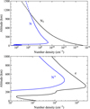 |
Fig. 1 Vertical density profiles of N2 and N (top) and N+ and electrons (bottom) in Triton’s atmosphere and ionosphere from the surface to 1000 km, adapted from the model results of Krasnopolsky (2023). The densities of N2 and N are extrapolated to 1500 km (dashed lines) assuming diffusive equilibrium. |
2.2 Plasma environment
Voyager 2’s flyby provided key observations that significantly advanced our understanding of Neptune’s magnetospheric environment. Triton, orbiting at a distance of 14.3 Neptune radii, serves as a significant source of plasma for Neptune’s magnetosphere. Measurements from the low-energy charged particle (LECP) instrument on board Voyager 2 revealed a sharp decline in energetic ion intensity beyond Triton’s orbit (Krimigis et al. 1989; Mauk et al. 1991, 1994), indicating that plasma is predominantly generated near Triton’s orbit and subsequently transported inward (Eviatar et al. 1995). Measurements from the Voyager plasma science experiment identified two distinct ion populations: a light species, likely protons, and a heavier species, presumed to be atomic nitrogen ions (Belcher et al. 1989; Richardson et al. 1990). This composition supports the hypothesis that hydrogen and nitrogen atoms escaping from Triton populate gravitationally bound orbits around Neptune (Summers & Strobel 1991), forming an extended neutral cloud known as the Triton torus.
Observations from the Voyager 2 encounter revealed that Neptune’s magnetic dipole is significantly tilted by 47° and offset from the planet’s center (Ness et al. 1989; Connerney et al. 1991). Combined with Triton’s highly inclined retrograde orbit (158°), this geometry leads to a highly variable magnetospheric plasma environment along Triton’s orbital path. Previous studies suggested that as Triton traverses Neptune’s magnetosphere across L shells ranging from ~14 to beyond 40, the ambient plasma number density varies from 10−4 to 10−1 cm−3 due to periodic changes in its distance to the central plasma sheet (Richardson & McNutt 1990; Strobel et al. 1990a; Richardson 1993; Zhang et al. 1991). Voyager 2 measurements indicated that heavy ions were detected only when Triton crossed the plasma sheet, with the local plasma composed of N+ at energies around 65 eV and H+ at energies at 7 eV (Belcher et al. 1989). Based on the offset tilted dipole model of Ness et al. (1989), Richardson et al. (1990) further showed that Triton spends approximately 22% of its orbit inside L = 15 and another 22% between L = 15 and 17. These regions are characterized by relatively high plasma fluxes, beyond which the plasma fluxes drop off sharply (Krimigis et al. 1989, 1990). Within these inner L-shell regions, magnetospheric protons are accelerated to energies of several tens of keV, representing a significant source of ionization and potential atmospheric sputtering for Triton.
Accordingly, we adopted an incident plasma population composed of N+ and H+ with characteristic energies of 65 eV and 7 eV, respectively. To assess the sensitivity of atmospheric responses to varying plasma conditions, an additional N+ population with energies ranging from 60 eV to 140 eV was included. An average N+ flux of 1.2×105 cm−2 s−1 is adopted based on Lammer (1995). In addition, we considered a second population of energetic protons to represent conditions when Triton resides within Neptune’s inner L shell region. Their differential energy spectrum, ranging of 1–100 keV, was derived from Voyager LECP measurements and follows a hot Maxwellian distribution with a characteristic temperature of 62 keV (Krimigis et al. 1990), as shown in Fig. 2. It is important to note that, due to the limited observational coverage of the Voyager 2 flyby, the actual ion precipitation flux onto Triton remains poorly constrained. Therefore, the ion fluxes employed in this study should be regarded as reference estimates based on locally observed plasma properties near Triton. Among the various ion populations considered, our subsequent simulations indicate that the precipitation of low-energy (7 eV) protons exerts a negligible influence on Triton’s atmosphere. Therefore, this component is omitted from detailed discussion in the following sections.
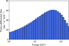 |
Fig. 2 Differential energy spectrum of protons adapted from the LECP measurements, representing energetic proton precipitation when Triton is located within Neptune’s inner L shell region. The proton energy distribution is characterized by a Maxwellian profile with a temperature of 62 keV (Krimigis et al. 1990). |
2.3 Monte Carlo calculations
The precipitation of magnetospheric ions into Triton’s atmosphere initiates a range of collisional interactions, including both elastic and inelastic processes. The latter include charge exchange, dissociation, ionization, and excitation. Furthermore, such interactions can result in the production of energetic secondary particles capable of overcoming the gravitational binding energy of Triton’s atmosphere, thereby inducing atmospheric sputtering escape. To quantitatively assess this escape mechanism, the sputtering yield is defined as the average number of escaping atmospheric particles produced per incident ion (Johnson 1994). Given the stochastic nature of ion-neutral collisions and the potentially involved atmospheric recoils (secondary atoms and/or molecules ejected by energetic particles), Monte Carlo methods are particularly well suited for calculating sputtering yields. This approach has been extensively employed in prior investigations of sputter-induced atmospheric loss on planetary bodies, including Mars and Venus (Chaufray et al. 2007; Wang et al. 2014; Curry et al. 2025), and on satellites such as Io (McGrath & Johnson 1987; Pospieszalska & Johnson 1996) and Titan (Shematovich et al. 2003; Gu et al. 2019; Snowden & Higgins 2021). In addition, the Monte Carlo framework facilitates the simultaneous simulation of the energy degradation of incident ions as they undergo successive collisions with ambient neutrals, thereby enabling a comprehensive treatment of the associated collisional processes and their cumulative effects on the ionization of Triton’s atmosphere.
Modified from our existing atmospheric sputtering model (Gu et al. 2019, 2023; Huang et al. 2024), a one-dimensional test particle Monte Carlo model is employed to simulate the precipitation of energetic ions and the resulting atmospheric recoils on Triton. A plane-parallel background atmosphere is adopted, based on the neutral density profiles presented in Fig. 1, which is assumed to present a global average of Triton’s atmosphere. The lower boundary is defined at Triton’s surface and is treated as an absorbing boundary, that is, particles reaching this surface are assumed to condense without reflection and are therefore excluded from further tracking. The upper boundary is set at an altitude of 1500 km, above which the collision probabilities drop to less than 0.1%. This ensures that the atmospheric region above this limit does not significantly affect the calculation of sputtering yields. The entire background atmosphere of Triton is divided into 50 vertical grids, each with a depth of 30 km. The incident plasma population comprises N+ and H+, with their respective initial energy distributions described in Sect. 2.2. For N+, only elastic scattering and charge exchange are considered, as its characteristic energy lies well below the thresholds for other inelastic processes. In contrast, energetic H+ ions with keV-level energies are subject to additional dissociation, ionization, and excitation reactions. The relevant dissociation and ionization reactions incorporated in the simulations, along with their corresponding energy losses, are summarized in Table 1. Ionization of atomic N is excluded from consideration owing to the lack of reliable cross section measurements. For energy losses due to electronic excitation, ΔEe (in units of eV), we adopted the empirical formula derived by Firsov (1959):
![Mathematical equation: \bigtriangleup E_e = \frac{4.3\times 10^{-8} v (Z_A+Z_B)^{5/3}}{[1+0.3b(Z_A+Z_B)^{1/3}]^5 },](/articles/aa/full_html/2025/10/aa56273-25/aa56273-25-eq1.png) (1)
(1)
where b is the impact parameter in units of Bohr radius, v is the relative velocity in units of cm s−1, and ZA and ZB are nuclear charge numbers of the impacting and target species, respectively.
In each independent model run, ions are initiated at the top of Triton’s atmosphere with a specified incident energy and incidence angle. Their trajectories are tracked under the influence of Triton’s gravity until the occurrence of a collision, which is determined by the following expression:
 (2)
(2)
where Δz is the vertical length scale used to perform the integration, σi and ni are the total collision cross section and number density of species i (N2 and N), respectively, β is the angle between the impacting particle’s velocity and vertical downward, and R1 is a random number between 0 and 1. The influence of electromagnetic fields is not included in the calculations, as the ion energies considered in this study (e.g., 1–100 keV protons) correspond to large gyroradii (typically >1000 km), which are much larger than the relevant atmospheric scale heights (e.g., ~100 km for N2 at exobase). The ambient neutrals are assumed to be stationary prior to collision, as their thermal velocities are negligible compared to the energies of incident ions. The implementation of the collision scheme, including scattering parameter (αE) determination, is described in Appendix A.
The above procedure is iteratively applied until one of the following termination criteria is met: (1) the kinetic energy of the incident ion drops below the local escape energy during its energy degradation process, rendering it incapable of further contributing to atmospheric escape; (2) the ion either becomes fully thermalized upon reaching the surface or escapes through the upper boundary of the simulation domain. All secondary recoils of background species generated throughout the cascade of collisions are tracked using the same procedure as that applied to the primary incident ions.
To calculate the local energy deposition rate, we tracked the total kinetic energy lost (∆Et) by both the impacting particle (a) and the target particle (b) during each collision. For the impacting particle, the local energy loss is given by the difference between its pre- (Ea0) and post-collision (Ea1) kinetic energies. However, part of this energy is transferred to the target particle, which can subsequently migrate away from the collision site. Therefore, the net energy deposited locally at the point of collision is calculated as
 (3)
(3)
where Eb1 is the kinetic energy acquired by the target particle after the collision. Both the impacting and target particles are subsequently tracked throughout their trajectories until they satisfy the termination criteria described earlier.
Dissociation and ionization reactions considered in the simulations for energetic proton precipitation.
3 Results
3.1 Sputtering yield and escape rate
We present in Fig. 3 the sputtering yields of N2 and N induced by N+ precipitation, as functions of incidence angle (0°-80°) and incident energy (60–140 eV), assuming three representative scattering angle distributions: strong forward scattering (αE = –1.5), isotropic scattering (αE = 0.01), and backscattered (αE = 1.5). An incidence angle of 0° corresponds to precipitating ions enter the atmosphere perpendicularly. Several key features are evident from the figure.
First, our calculations indicate that the sputtering yields range from 0.15 to 31.78 for N2, and from 0.13 to 9.26 for N, both resulting from incident N+ ions. In all cases, sputtering yields increase with both incidence angle and energy. For instance, under strong forward scattering conditions, the sputtering yields of N2 increase from 0.15 to 5.07 as the incident angle varies from 0° to 80° at a given energy of 60 eV, and from 0.19 to 10.75 at 140 eV. This behavior is consistent with the fact that ions with higher kinetic energies tend to produce more atmospheric recoils along their energy degradation processes (Lammer 1995; Johnson et al. 2000). Meanwhile, oblique incidence angles confine the ion and recoil trajectories to the upper atmosphere, where the escape probability is higher due to the reduced atmospheric density (Gu et al. 2019, 2023).
Second, sputtering yields increase with increasingly αE (i.e., transitioning from forward to backward scattering). At an incident energy of 65 eV and an angle of 80°, the N2 sputtering yields are 5.14, 16.78, and 17.94 for scattering parameters of –1.5, 0.01, and 1.5, respectively. This trend can be attributed to the increased efficiency of energy transfer from the incident ions to background neutrals under backward scattering conditions, resulting in more energetic atmospheric recoils capable of escaping Triton (Huang et al. 2024).
Third, N2 sputtering yields are consistently higher than those of atomic N, reflecting the dominant abundance of N2 in Triton’s atmosphere. For example, at an incident energy of 120 eV and an angle of 80°, the sputtering yield of N under forward scattering is 5.32, roughly half of the corresponding N2 yield under the same conditions. In addition, low-energy population of protons with 7 eV results in negligible the sputtering yields compared to those bombarded by incident N+. Hence, our study did not account for its role in modulating atmospheric escape processes or Triton’s ionospheric structure.
When orbiting inside Neptune’s inner L shell regions, Triton experiences energetic proton precipitation with energies of tens of keV (Krimigis et al. 1990). Figure 4 illustrates the N2 and N sputtering yields bombarded by H+ with a wide range of incident energy, varying from 1 keV to 100 keV, and incidence angles from 0°-80°, for three scattering angle distributions (the same as for N+ precipitation). Similar overall trends are observed for H+−induced sputtering, which depends positively on both incident energy and incidence angle, and is further increased under backward scattering conditions. Specifically, under forward scattering condition, N2 sputtering yields increase from 2.95 to 259.88 as the incident energy rises from 1 to 100 keV at normal incidence, and reach up to 668.50 at 80°. Backward scattering leads to substantially higher yields, especially at higher energies and angles. At 100 keV with normal incidence, isotropic and backward scattering produce yields that are approximately 3.9 and 13.6 times greater than those under forward scattering, respectively. Compared to N+ precipitation, incident H+ ions, despite their lower masses, generate more atmospheric recoils due to their higher velocities relative to the heavier but slower-moving nitrogen ions. As a result, the corresponding sputtering yields can exceed several thousand.
Based on our model results, two populations of incident ions are found to be effective in driving atmospheric sputtering at Triton: N+ with energies of 60-140 eV and H+ with energies ranging of 1–100 keV. The hemispheric sputtering rate (in units of s−1),  , at the exobase for species, i (N2 or N), induced by energetic ions, j (N+ or H+), can be calculated via
 (4)
(4)
where RTriton = 1353 km is the solid body radius of Triton, zexo = 870 km is the assumed exobase altitude, θ is the plasma incidence angle, and Φ is the incident flux of N+ or H+ (as described in Sect. 2.2).
Figure 5 presents the N2 and N escape rates induced by N+ and H+ precipitation as functions of incident energy, under forward, isotropic, and backward scattering conditions (αE = −1.5, 0.01, and 1.5, respectively). According to our calculations, the total escape rates are 2.2×10²¹−8.0×1025 s−1 for N2 and 1.2×10²¹−2.2×1025 s−1 for N, respectively. For both species, the escape rate increases positively with incident energy and scattering parameter, and the tendency becomes more pronounced at higher energies. To be more specific, the escape rates of N2 induced by N+ increase from 6.90×1024 s−1 to 1.25×1025 s−1 (for αE = −1.5), from 2.88×1025 s−1 to 5.32×1025 s−1 (for αE = 0.01), and from 4.38×1025 s−1 to 8.03×1025 s−1 (for αE = 1.5), as the incident energy increasing from 60 eV to 140 eV. In all cases, the escape rate of N2 consistently exceeds that of N, primarily due to its higher atmospheric abundance. Although H+ precipitation leads to higher sputtering yields, the substantially higher flux of N+ results in overall higher escape rates. For instance, the H+−induced escape rate of N2 spans from 2.16×10²¹ s−1 to 5.94×1024 s−1, which is 1-3 orders of magnitude lower than that induced by N+. This highlights the dominant contribution of N+ precipitation to atmospheric loss from Triton.
Atmospheric sputtering induced by ion precipitation on Triton has been investigated in several previous studies, reporting a wide range of escape rates depending on the adopted methods and assumptions. For example, Richardson et al. (1990) estimated an N2 escape rate of 2×10²¹ s−1 induced by pure proton precipitation, assuming a sputtering yield of three based on laboratory experiments by Brown et al. (1982) on water ice. Using an analytical model, Lammer (1995) predicted an average N2 escape rate of approximately 3×1024 to 1×1025 s−1 for N+ precipitation with an incidence angle of 80°-85° and energies between 65 eV and 120 eV. This is comparable to our model results, which range from 6.9 × 1024 to 8.03 × 1025 s−1 under similar conditions. For H+ precipitation with incidence angles exceeding 60° and energies around 50 keV, their estimated escape rates are on the order of ~1023 s−1, consistent with our results of ~1023 to 1024 s−1. Our model tends to produce slightly higher escape rates than those reported by Lammer (1995), which may be due to differences in sputtering yield determination methods and variations in the assumed background atmospheric profiles (Huang et al. 2024). Nevertheless, the results remain in good overall agreement with previous studies.
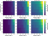 |
Fig. 3 Distributions of N2 and N sputtering yields induced by incident N+, shown as functions of incidence angle and incident energy. The left, middle, and right columns corresponds to three representative scattering angle distributions, characterized by the scattering parameter αE = −1.5 (strong forward scattering), αE = 0.01 (isotropic scattering), and αE = 1.5 (backscattered). |
3.2 Energy deposition, charge exchange, and ionization rates
Figure 6 presents energy deposition rates (top row) and charge exchange rates (bottom row) for incident N+ under varying scattering parameters (αE = –1.5, –0.5, 0.01, 0.5, 1.5), incident energies (60-140 eV), and incidence angles (0°-80°). At an incident energy of 120 eV and an incidence angle of 55° (Fig. 6a), increasing αE results in a reduction of the peak energy deposition rate from 1.49 to 0.52 eV cm−3 s−1, while the peak altitude shifts upward from 360 km to 600 km. Besides, a similar trend is observed with increasing incidence angle (Fig. 6b), when incident energy remains 120 eV and αE is fixed at –0.5. The peak rate declines from 1.03 to 0.38 eV cm−3 s−1, accompanied by an increase in peak altitude from 420 km to 570 km. These behaviors can be attributed to the fact that, under more oblique incidence or backward scattering conditions, ions are more likely to deposit their energy at higher altitudes, where the ambient atmospheric density is lower and fewer collisions occur. Moreover, under the same incidence angle of 55° and αE = −0.5 (Fig. 6c), increasing the incident energy from 60 to 140 eV enhances the peak deposition rate by a factor of approximately 2.2, while the peak altitude remains nearly unchanged. This is expected, as ions with higher initial energies can penetrate deeper into the atmosphere and interact more efficiently with background species, resulting in a modest enhancement of the overall energy deposition.
The charge exchange rate shows overall trends consistent with those of the energy deposition rate. Specifically, as αE increases from −1.5 to 1.5, the peak value decreases from 5.32×10⁻³ to 4.47×10⁻³ cm−3 s−1, while the peak altitude rises from 570 km to 660 km (Fig. 6d). A similar pattern is observed with incidence angle (Fig. 6e). Increasing the incidence angle from 0° to 80° lowers the peak rate from 5.58×10⁻³ to 3.86×10⁻³ cm−3 s−1 and elevates the peak altitude by 240 km. Variations with ion energy are minimal (Fig. 6f). The peak rate changes slightly from 4.99×10⁻³ to 5.27×10⁻³ cm−3 s−1, with a corresponding altitude decrease by 30 km. Notably, in all cases, the peak altitude of the charge exchange rate is higher than that of the energy deposition rate, reflecting the greater likelihood of charge exchange occurring at higher energies and altitudes.
Similarly, energy deposition, charge exchange, and ionization rates of incident H+ are presented in Fig. 7. We conducted identical sensitivity tests as those performed for N+ precipitation, systematically varying the scattering parameter, incidence angle, and incident energy (1–100 keV). We note here that dissociation rate is not presented because of its relative small contribution compared to the ionization processes. In general, the variations in energy deposition, charge exchange, and ionization rates induced by incident H+ ions follow similar trends to those observed for N+ precipitation, with several distinguishing features summarized as follows.
First, at a 55° incidence angle and a scattering parameter of αE = −0.5 (Fig. 7c), increasing proton energy from 1 to 100 keV leads to a substantial enhancement in energy deposition. The peak value increases by almost four orders of magnitude, from 5.38×10⁻⁴ to 4.84 eV cm−3 s−1, while the altitude of maximum deposition drops from 390 km to 240 km. Interestingly, once the incident energy exceeds approximately 20 keV, protons possess sufficient kinetic energy to undergo multiple collisional interactions while retaining enough residual energy to penetrate into Triton’s lower atmosphere and potentially reach the planetary surface.
Second, the charge exchange rate is highly sensitive to proton energy (Fig. 7f), predominantly due to variations in incident flux across the energy range. As energy increases, the peak rate amplifies by over two orders of magnitude (from 9.77×10⁻⁸ to 2.97×10⁻⁵ cm−3 s−1), while the corresponding altitude shows a slight downward shift.
Third, ionization only becomes significant above 10 keV, aligning with the energy threshold adopted for ionization collisions in this study (10–100 keV; see Fig. B.1). For example, under forward scattering (αE = −0.5), a 50 keV proton at 55° incidence angle yields a peak ionization rate of 0.031 cm−3 s−1 at around 360 km. It should be noted that this finding is constrained by the current lack of laboratory cross section data within the relevant energy regime. Improved experimental measurements are essential for more robust characterization of ionization processes in Triton’s upper atmosphere.
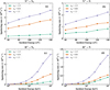 |
Fig. 5 N2 and N escape rates induced by magnetospheric N+ (upper panels) and H+ (lower panels) precipitation as functions of incident energy, ranging from 60-140 eV for N+ and 1-100 keV for H+. Results are shown for three scattering angle distributions corresponding to strong forward (αE = −1.5), isotropic (αE = 0.01), and backward (αE = 1.5) scattering conditions. |
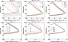 |
Fig. 6 Energy deposition and charge exchange rates for incident N+ under varying scattering parameter assumptions (αE = −1.5, −0.5, 0.01, 0.5, and 1.5, left column), incident energy (60-140 eV, middle column), and incidence angle (0°-80°, right column). The corresponding model parameters are indicated in each panel title. |
4 Discussion
4.1 Comparison with other atmospheric escape mechanisms
It is instructive to compare our modeled sputtering-induced atmospheric escape rates with those associated with other escape mechanisms. Previous studies have estimated the Jeans escape rates for atomic N and N2 to be on the order of 1024−1025 s−1 (Broadfoot et al. 1989; Krasnopolsky et al. 1993), while the combined escape rate of hydrogen species (H + H2) has been estimated to lie in the range (7-11)×1025 s−1 (Summers & Strobel 1991; Krasnopolsky & Cruikshank 1995). In contrast, the Jeans escape rates for heavier species such as atomic C and O are 2–3 orders of magnitude lower (Strobel et al. 1990b; Krasnopolsky & Cruikshank 1995). In addition, Gu et al. (2021a) evaluated nonthermal escape rates driven by atmospheric and ionospheric chemistry, showing that chemically induced escape of atomic N and O can also be significant, with rates of 8.0 × 1024 s−1 and 1.4 × 10²³ s−1, respectively. The contributions from atomic H and C were found to be smaller but non-negligible. Our results show that N2 and atomic N escape induced by N+ sputtering ranges from ~1024 to 1025 s−1, while that induced by H+ precipitation spans a broader range from ~1021 to 1024 s−1. These values place the sputtering-driven escape rate of nitrogen on par with both the Jeans escape rate and the chemical escape rate reported in previous studies, highlighting the important role of energetic ion precipitation in driving atmospheric loss from Triton.
4.2 Proton precipitation as an ionization source
In this study, we examined the impact of magnetospheric proton precipitation on Triton’s ionosphere by incorporating seven key dissociation (coupled with charge exchange) and ionization reactions (listed in Table 1). Figure 8 illustrates the dissociation and ionization rates associated with these reactions, assuming incident H+ ions with an energy of 50 keV, an incidence angle of 55°, and a scattering parameter of −0.5. Among all reactions, Reaction 4 (H+ + N+ + e) dominates, contributing an integrated column rate of 2.5× 104 cm−2 s−1, approximately 40% of the total ionization. Reactions 5 (H+ + N+ + N + e) and 6 (H+ + N+ + N+ + 2e) also make substantial contributions, jointly accounting for 30% of the total. We observe a clear positive correlation between the contribution of each reaction and its corresponding collision cross section; this highlights the increased likelihood of reactions with larger cross sections due to the higher probability of interactions between incident protons and background species.
To further assess the relative importance of ion precipitation, we compared our modeled results with two other major ionization sources in Triton’s atmosphere: solar EUV radiation and magnetospheric electron precipitation. Figure 9 presents the ionization rate profiles driven by these three sources. In our model, the total ionization rate (N + N+) induced by ion precipitation is obtained by simulating protons with energies ranging from 10 to 100 keV, assuming an incidence angle of 55° and αE = −1.5. An incidence angle of 55° is adopted to approximate the average incidence angle of ion precipitation over a hemisphere, while αE = −1.5 characterizes a common strongly forward-scattering angle distribution (Kharchenko et al. 2000; Gacesa et al. 2020). The fluxes are normalized according to the observed proton energy spectrum. For comparison, Fig. 9 includes ionization rates driven by solar EUV and magnetospheric electron precipitation from Strobel et al. (1990a), and rates from magnetospheric electron impact modeled by Benne et al. (2024).
Previous studies have consistently identified magnetospheric electron precipitation as the primary driver of ionization in Triton atmosphere (Majeed et al. 1990; Summers & Strobel 1991; Strobel & Zhu 2017). According to Strobel et al. (1990a), magnetospheric electron precipitation yields a peak ionization rate of 15 cm−3 s−1 at approximately 250 km, while solar EUV radiation produces a peak rate about one order of magnitude lower, centered around 420 km. In a recent study, Benne et al. (2024) accounted for the additional contribution of photoelectrons and adopted a lower incident flux of magnetospheric electrons, and derived electron density profiles that are consistent with Voyager 2 observations. Notably, they identified a double-peak structure in the ionization profiles: one peak near 400 km driven by photoelectrons, and another near 71 km caused by magnetospheric electron impact. The maximum secondary electron production rate is 1.82 cm−3 s−1, roughly an order of magnitude lower than that reported by Strobel et al. (1990a). For comparison, our model predicts a peak ionization rate of 0.4 cm−3 s−1 at 300 km, driven by ion precipitation, which is 1–2 orders of magnitude lower than that reported in previous studies.
Our calculations suggest a column-integrated ionization rate of 3.9×106 cm−2 s−1. For comparison, Benne et al. (2024) reported a total column rate of 2.8×107 cm−2 s−1. The estimates from Strobel et al. (1990a) yield column rates on the order of ~107 cm−2 s−1 for solar EUV and ~108 cm−2 s−1 for magnetospheric electron precipitation. Moreover, as suggested by Krasnopolsky & Cruikshank (1995), the column ionization rate of (N2+ + N+) was estimated to be 6.9×107 cm−2 s−1 due to magnetospheric electron ionization, compared to 2.9×107 cm−2 s−1 from photo- and photoelectron ionization.
In summary, these comparisons suggest that while ion precipitation does contribute to ionization in Triton’s atmosphere, its effect is generally weaker than that of magnetospheric electron. This discrepancy arises partly from the higher fluxes of magnetospheric electrons observed by Voyager 2 (Krimigis et al. 1990). In addition, electrons are intrinsically more efficient at driving ionization due to several factors: they possess larger ionization cross sections, lower reaction thresholds, and higher energy transfer efficiency per collision due to their smaller mass. In contrast, ions tend to dissipate energy through various competing processes such as elastic scattering, charge exchange, dissociation, and excitation, diminishing the energy available for ionization and thereby limiting their overall contribution to ion production. These physical distinctions highlight the dominant role of electron precipitation in shaping Triton’s ionospheric structure.
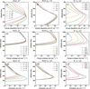 |
Fig. 7 Same as Fig. 6 but for the energy deposition, charge exchange, and ionization rates driven by incident H+. |
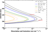 |
Fig. 8 Profiles of dissociation and ionization rates in Triton’s atmosphere resulting from the seven reactions studied in this work. Solid lines represent individual reaction contributions and the dashed line the total rate. All profiles result from an incident H+ population with an energy of 50 keV, an incidence angle of 55°, and a scattering parameter of –0.5. Red horizontal lines mark the altitudes corresponding to the peak densities of electron (solid, 330 km) and N+ (dashed, 460 km) for reference. |
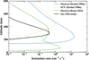 |
Fig. 9 Ionization rate profiles in Triton’s atmosphere induced by three energy sources: solar EUV radiation, magnetospheric electron precipitation, and magnetospheric ion precipitation. The black curve represents our simulation results for ion-driven ionization For comparison, ionization rates from previous studies are shown: solar EUV-driven (orange) and electron-driven (blue) ionization from Strobel et al. (1990a), and electron-driven ionization (green) from Benne et al. (2024). |
4.3 Model limitation
Several assumptions in our model introduce uncertainties into the results. First, we adopted magnetospheric ion fluxes from Voyager 2 LECP measurements, which may overestimate the actual precipitation flux reaching Triton’s atmosphere, as the transition from magnetospheric to precipitating flux remains poorly constrained. Second, the limited availability of laboratory data on collisional cross sections and scattering angle distributions between incident ions and atmospheric neutrals introduces additional uncertainty in the final results. Moreover, although ion precipitation can trigger a wide range of chemical reactions, our model includes only a subset of possible processes, likely leading to an underestimation of the total ionization impact. Improved laboratory measurements of key collision parameters are essential to better constrain these effects. Third, the use of a one-dimensional plane-parallel atmospheric structure introduces uncertainty by neglecting horizontal density variations. In addition, this assumption may result in underestimations, particularly when energetic recoils escape at large inclination angles relative to the vertical (Johnson et al. 2000; Gu et al. 2021b). Moreover, the current observational constraints on Triton’s atmosphere are extremely limited. Voyager 2 provided only brief flyby measurements with restricted spatial coverage, and no in situ ionospheric data are available to characterize latitudinal or longitudinal variability. While some modeling efforts suggest potential asymmetries related to surface frost distribution or solar illumination (Merlin et al. 2018; Marques Oliveira et al. 2022), these features remain poorly constrained. As such, the adoption of a one-dimensional structure offers a first-order approximation to the vertical ionization processes. Our results are restricted to atmospheric conditions representative of the Voyager 2 epoch. Later stellar occultation measurements suggest that Triton’s surface pressure increased by up to a factor of 2 by 2009 (Sicardy et al. 2024), which could enhance neutral densities and thus affect the total ionization rates. Fourth, the assumption of an absorbing boundary may lead to further underestimations of escape rates due to the fact that secondary sputtering contributions from ion-surface interactions are neglected (Johnson & Brown 1982). Finally, the exclusion of low-energy (7 eV) proton precipitation, despite its limited direct impact, may contribute to a cumulative underestimation of the overall model results. Nevertheless, our calculations highlight the significant contribution of magnetospheric ion precipitation to atmospheric escape and ionospheric processes on Triton.
5 Conclusions
We evaluated the magnetospheric ion precipitation into Triton’s upper atmosphere using a one-dimensional test particle Monte Carlo approach. The background atmosphere, primarily composed of N2 and N, was constructed based on a photochemical model of Krasnopolsky (2023) and was assumed to be plane-parallel. Precipitating N+ and H+ fluxes were derived from Lammer (1995) and Voyager 2 LECP measurements (Krimigis et al. 1990), respectively. We simulated the ion energy degradation process, considering various interactions between incident ions and the ambient neutrals via elastic scattering, charge exchange, dissociation, ionization, and excitation reactions. These processes modify Triton’s ionospheric structure and can energize atmospheric particles to escape velocities, contributing to atmospheric sputtering. We calculated the sputtering yields and escape rates of N2 and N, as well as the energy deposition, charge exchange, and ionization rates induced by magnetospheric N+ and H+, under various scattering parameter conditions (αE = −1.5, −0.5, 0.01, 0.5, and 1.5), incidence angles (0°-80°), and incident energies (60-140 eV for N+ and 1-100 keV for H+). The simulation results are summarized as follows.
First, the sputtering yields of N2 range from 0.13 to 31.78 for incident N+ and from ~3 to several thousand for incident H+, increasing with incident energy, incidence angle, and scattering parameter. The corresponding sputtering rates are on the order of 1024−1025 s−1 driven by N+ and 1021−1024 s−1 driven by H+, comparable to other escape mechanisms such as Jeans escape (Krasnopolsky et al. 1993) and chemical escape (Krasnopolsky & Cruikshank 1995; Gu et al. 2021a); this indicates that magnetospheric ion-driven sputtering is a significant contributor to Triton’s atmospheric loss. N yields are smaller due to its lower atmospheric abundance.
Second, energy deposition, charge exchange, and ionization rates exhibit similar dependences on the model inputs: their peak values (peak altitudes) increase (decrease) with incident energy. In contrast, an increasing incidence angle or scattering parameter reduces the peak magnitudes and shifts the peak altitude upward. Notably, H+ ions with energies exceeding 20 keV can retain sufficient energy after multiple collisions to penetrate into the lower atmosphere and, in some cases, reach Triton’s surface.
Third, of the ionization processes, H+ + N2 → H+ + N2+ + e is identified as the dominant channel, contributing approximately 40% of the total ionization; two other reactions (H+ + N2 → H+ + N+ + N + e and H+ + N2 → H+ + N+ + N+ + 2e) jointly account for an additional 30%. We further compared our modeled ionization rates with previous results for solar EUV and magnetospheric electron precipitation (Strobel et al. 1990a; Benne et al. 2024). Although weaker than electron precipitation, proton-induced ionization represents a non-negligible component of Triton’s ionospheric processes.
Finally, despite certain limitations in our calculations, our results highlight the role of ion precipitation as a complementary mechanism in shaping Triton’s upper atmospheric composition and escape. Future laboratory measurements and multidimensional spherical modeling efforts are essential to refine our understanding of magnetospheric ion precipitation in Triton’s atmosphere.
Acknowledgements
The authors acknowledge supports from the National Natural Science Foundation of China through grants 42030201, 42261160643, 42241112, and 42475134.
Data availability
All model results and code are available at https://doi.org/10.6084/m9.figshare.29424629.v2
Appendix A Collisional scheme
The collision type (either elastic or inelastic) and collision partner (N2 or N) are selected stochastically based on the column density ratio between background species along the particle trajectory and the cross sections (see Appendix B for detailed reference of collisional cross sections utilized in this study) for different collisional processes. This selection is governed by a second random number R2. Following each collision, a scattering angle is assigned using another random number R3. Analogous to Kallio & Barabash (2000), the laboratory-frame scattering angle, θlab, is defined as
![Mathematical equation: \theta_{lab} = [R3 \cdot (\theta_{max}^{\alpha_E}-\theta_{min}^{\alpha_E})+\theta_{min}^{\alpha_E}]^{1/\alpha_E},](/articles/aa/full_html/2025/10/aa56273-25/aa56273-25-eq6.png) (A.1)
(A.1)
where αE is the scattering parameter, θmin is the minimum scattering angle assumed to be 1° to prevent an infinitely large cross section as the scattering angle approaches zero (Noël & Prölss 1993), and θmax is the maximum scattering angle, expressed as
 (A.2)
(A.2)
and ρm can be expressed as
 (A.3)
(A.3)
with ma and mb denoting the masses of the impacting and target particles, respectively, ∆Et the energy lost to inelastic processes, and Ea0 the pre-collision kinetic energy of the impacting particle. The center-of-mass scattering angle, θCM, is then computed as
![Mathematical equation: \theta_{CM} = \arccos\left[ -\rho_m+\rho_m\cos(\theta_{lab})^2+\cos(\theta_{lab})\sqrt{1-\rho_m^2 \sin(\theta_{lab})^2} \right].](/articles/aa/full_html/2025/10/aa56273-25/aa56273-25-eq9.png) (A.4)
(A.4)
Given the scarcity of comprehensive differential scattering cross section measurements, we followed the approach of Snowden & Higgins (2021) and employed five representative values of the scattering parameter αE (−1.5, −0.5, 0.01, 0.5, and 1.5) to systematically assess the model’s sensitivity to assumed scattering angle distributions. In this framework, negative values of αE correspond to highly forward scattering angle distributions, favoring small scattering angles. Values of αE near zero imply nearly isotropic scattering, while positive values indicate a preference for large scattering angles. Finally, the kinetic energies of the impacting and target particles after the collision are determined by applying the laws of energy and momentum conservation, with the inelastic energy loss subtracted before each collision.
Appendix B Collisional cross section
In this section we detail the binary collision cross sections employed in this study. Figure B.1 presents the elastic, charge exchange, dissociation, and ionization cross sections as functions of relative collision energy. The elastic cross sections for N+ZN2ZN-N2 were adapted from Snowden & Higgins (2021) and those for H+∕H-N2 from Noël & Prölss (1993). The charge exchange cross sections for H+−N2 are obtained from Lindsay & Stebbings (2005). Dissociation and ionization cross sections for H+−N2 collisions follow the data presented in Luna et al. (2003). Due to the absence of comprehensive laboratory measurements, elastic and charge exchange cross sections involving atomic nitrogen with either incident ions or background neutrals are not available. In such cases, we employed estimated values derived from hard-sphere approximations combined with energy dependences derived from existing datasets. For example, the elastic cross sections for N+−N were approximated as 0.21 times that of N+−N2, where 0.21 corresponds to the ratio of the hard-sphere cross sections between the N+−N and N+−N2. The hard-sphere radii used for estimation, corresponding to the relevant neutral and ionic species, are summarized in Table B.1. Additionally, for H+/H-N2 elastic cross sections, analytical fits derived from the semi-empirical formulation by Lewkow et al. (2012) are applied to extrapolate values into the low-energy regime (1–100 eV), where direct measurements are unavailable. The fitting follows the functional form
 (B.1)
(B.1)
where E0 is set to 1 keV, and σ0 and β are fitting parameters determined from the available data. The best-fit values of σ0 and β are 2.17×10⁻¹⁶ and 0.63 for H+−N2 collisions, and 2.03×10⁻¹⁶ and 0.66 for H-N2 collisions, respectively.
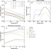 |
Fig. B.1 Energy-dependent elastic, charge exchange, dissociation and ionization cross sections considered in this study. In panel (a), analytical fits for H+/H-N2 elastic cross sections, based on the semi-empirical formula of Lewkow et al. (2012), are shown as dashed lines. |
Hard sphere radii for the neutral and ionic species used in this study.
References
- Belcher, J. W., Bridge, H. S., Bagenal, F., et al. 1989, Science, 246, 1478 [Google Scholar]
- Benne, B., Benmahi, B., Dobrijevic, M., et al. 2024, A&A, 686, A22 [NASA ADS] [CrossRef] [EDP Sciences] [Google Scholar]
- Broadfoot, A. L., Atreya, S. K., Bertaux, J. L., et al. 1989, Science, 246, 1459 [NASA ADS] [CrossRef] [Google Scholar]
- Brown, W. L., Lanzerotti, L. J., & Johnson, R. E. 1982, Science, 218, 525 [NASA ADS] [CrossRef] [Google Scholar]
- Chaufray, J. Y., Modolo, R., Leblanc, F., et al. 2007, J. Geophys. Res. (Planets), 112, E09009 [Google Scholar]
- Clementi, E., & Raimondi, D. L. 1963, J. Chem. Phys., 38, 2686 [Google Scholar]
- Connerney, J. E. P., Acuna, M. H., & Ness, N. F. 1991, J. Geophys. Res., 96, 19023 [Google Scholar]
- Conrath, B., Flasar, F. M., Hanel, R., et al. 1989, Science, 246, 1454 [NASA ADS] [CrossRef] [Google Scholar]
- Cravens, T. E., Robertson, I. P., Ledvina, S. A., et al. 2008, Geophys. Res. Lett., 35, L03103 [Google Scholar]
- Curry, S. M., Hara, T., Luhmann, J. G., et al. 2025, Sci. Adv., 11, eadt1538 [Google Scholar]
- De La Haye, V., Waite, J. H., Cravens, T. E., et al. 2007, Icarus, 191, 236 [Google Scholar]
- Dutuit, O., Carrasco, N., Thissen, R., et al. 2013, ApJS, 204, 2, 20 [Google Scholar]
- Eviatar, A., Vasyliu¯ nas, V. M., & Richardson, J. D. 1995, J. Geophys. Res., 100, 19551 [Google Scholar]
- Fang, X., Bougher, S. W., Johnson, R. E., et al. 2013, Geophys. Res. Lett., 40, 1922 [NASA ADS] [CrossRef] [Google Scholar]
- Firsov, O. B. 1959, Sov. J. Exp. Theor. Phys., 9, 1076 [Google Scholar]
- Fox, J. L., & Hac´, A. B. 2018, Icarus, 300, 411 [NASA ADS] [CrossRef] [Google Scholar]
- Gacesa, M., Lillis, R. J., & Zahnle, K. J. 2020, MNRAS, 491, 4, 5650 [Google Scholar]
- Gu, H., Cui, J., Niu, D.-D., et al. 2019, A&A, 623, A18 [NASA ADS] [CrossRef] [EDP Sciences] [Google Scholar]
- Gu, H., Cui, J., Niu, D.-D., et al. 2021a, A&A, 650, A130 [NASA ADS] [CrossRef] [EDP Sciences] [Google Scholar]
- Gu, H., Cui, J., Niu, D., et al. 2021b, MNRAS, 501, 2394 [NASA ADS] [CrossRef] [Google Scholar]
- Gu, H., Wu, X., Huang, X., et al. 2023, ApJ, 959, 80 [Google Scholar]
- Huang, X., Gu, H., Cui, J., et al. 2023, J. Geophys. Res. (Planets), 128, e2023JE007811 [Google Scholar]
- Huang, X., Gu, H., Ni, Y., et al. 2024, J. Geophys. Res. (Planets), 129, e2023JE008129 [Google Scholar]
- Ip, W.-H. 1990, Geophys. Res. Lett., 17, 1713 [Google Scholar]
- Johnson, R. E., & Brown, W. L. 1982, Nucl. Instrum. Methods Phys. Res., 198, 103 [Google Scholar]
- Johnson, R. E. 1994, Space Sci. Rev., 69, 215 [Google Scholar]
- Johnson, R. E., Schnellenberger, D., & Wong, M. C. 2000, J. Geophys. Res., 105, 1659 [Google Scholar]
- Johnson, R. E., Combi, M. R., Fox, J. L., et al. 2008, Space Sci. Rev., 139, 355 [CrossRef] [Google Scholar]
- Kallio, E., & Barabash, S. 2000, J. Geophys. Res., 105, 24973 [Google Scholar]
- Kharchenko, V., Dalgarno, A., Zygelman, B., et al. 2000, J. Geophys. Res., 105, A11, 24899 [Google Scholar]
- Krasnopolsky, V. A. 2023, Icarus, 406, 115741 [NASA ADS] [CrossRef] [Google Scholar]
- Krasnopolsky, V. A., & Cruikshank, D. P. 1995, J. Geophys. Res., 100, 21271 [NASA ADS] [CrossRef] [Google Scholar]
- Krasnopolsky, V. A., Sandel, B. R., & Herbert, F. 1992, J. Geophys. Res., 97, 11695 [NASA ADS] [CrossRef] [Google Scholar]
- Krasnopolsky, V. A., Sandel, B. R., Herbert, F., et al. 1993, J. Geophys. Res., 98, 3065 [NASA ADS] [CrossRef] [Google Scholar]
- Krimigis, S. M., Armstrong, T. P., Axford, W. I., et al. 1989, Science, 246, 1483 [NASA ADS] [CrossRef] [Google Scholar]
- Krimigis, S. M., Mauk, B. H., Cheng, A. F., et al. 1990, Geophys. Res. Lett., 17, 1685 [Google Scholar]
- Lammer, H. 1995, Planet. Space Sci., 43, 845 [Google Scholar]
- Leblanc, F., Modolo, R., Curry, S., et al. 2015, Geophys. Res. Lett., 42, 9135 [Google Scholar]
- Lellouch, E., Blanc, M., Oukbir, J., et al. 1992, Adv. Space Res., 12, 113 [Google Scholar]
- Lellouch, E., de Bergh, C., Sicardy, B., et al. 2010, A&A, 512, L8 [NASA ADS] [CrossRef] [EDP Sciences] [Google Scholar]
- Lewkow, N. R., Kharchenko, V., & Zhang, P. 2012, ApJ, 756, 57 [Google Scholar]
- Lindsay, B. G., & Stebbings, R. F. 2005, J. Geophys. Res. (Space Phys.), 110, A12213 [NASA ADS] [CrossRef] [Google Scholar]
- Lindal, G. F., Wood, G. E., Hotz, H. B., et al. 1983, Icarus, 53, 348 [Google Scholar]
- Liuzzo, L., Paty, C., Cochrane, C., et al. 2021, J. Geophys. Res. (Space Phys.), 126, e29740 [Google Scholar]
- Luhmann, J. G., & Kozyra, J. U. 1991, J. Geophys. Res., 96, 5457 [CrossRef] [Google Scholar]
- Luna, H., Michael, M., Shah, M. B., et al. 2003, J. Geophys. Res. (Planets), 108, 5033 [Google Scholar]
- Majeed, T., McConnell, J. C., Strobel, D. F., et al. 1990, Geophys. Res. Lett., 17, 1721 [NASA ADS] [CrossRef] [Google Scholar]
- Marques Oliveira, J., Sicardy, B., Gomes-Júnior, A. R., et al. 2022, A&A, 659, A136 [NASA ADS] [CrossRef] [EDP Sciences] [Google Scholar]
- Mauk, B. H., Keath, E. P., Kane, M., et al. 1991, J. Geophys. Res., 96, 19061 [Google Scholar]
- Mauk, B. H., Krimigis, S. M., & Acuna, M. H. 1994, J. Geophys. Res., 99, 14781 [Google Scholar]
- McGrath, M. A., & Johnson, R. E. 1987, Icarus, 69, 519 [Google Scholar]
- Merlin, F., Lellouch, E., Quirico, E., et al. 2018, Icarus, 314, 274 [NASA ADS] [CrossRef] [Google Scholar]
- Ness, N. F., Acuna, M. H., Burlaga, L. F., et al. 1989, Science, 246, 1473 [NASA ADS] [CrossRef] [Google Scholar]
- Noël, S., & Prölss, G. W. 1993, J. Geophys. Res., 98, 17317 [Google Scholar]
- Pospieszalska, M. K., & Johnson, R. E. 1996, J. Geophys. Res., 101, 7565 [Google Scholar]
- Richardson, J. D., Eviatar, A., & Delitsky, M. L. 1990, Geophys. Res. Lett., 17, 1673 [Google Scholar]
- Richardson, J. D. 1993, Geophys. Res. Lett., 20, 1467 [Google Scholar]
- Richardson, J. D., & McNutt, R. L. 1990, Geophys. Res. Lett., 17, 1689 [Google Scholar]
- Shematovich, V. I., Johnson, R. E., Michael, M., et al. 2003, J. Geophys. Res. (Planets), 108, 5087 [Google Scholar]
- Sicardy, B., Tej, A., Gomes-Júnior, A. R., et al. 2024, A&A, 682, L24 [NASA ADS] [CrossRef] [EDP Sciences] [Google Scholar]
- Sittler, E. C., & Hartle, R. E. 1996, J. Geophys. Res., 101, 10863 [Google Scholar]
- Slater, J. C. 1964, J. Chem. Phys., 41, 3199 [CrossRef] [Google Scholar]
- Snowden, D., & Higgins, A. 2021, Icarus, 354, 113929 [Google Scholar]
- Strobel, D. F., & Zhu, X. 2017, Icarus, 291, 55 [NASA ADS] [CrossRef] [Google Scholar]
- Strobel, D. F., Cheng, A. F., Summers, M. E., et al. 1990a, Geophys. Res. Lett., 17, 1661 [NASA ADS] [CrossRef] [Google Scholar]
- Strobel, D. F., Summers, M. E., Herbert, F., et al. 1990b, Geophys. Res. Lett., 17, 1729 [NASA ADS] [CrossRef] [Google Scholar]
- Summers, M. E., & Strobel, D. F. 1991, Geophys. Res. Lett., 18, 2309 [NASA ADS] [CrossRef] [Google Scholar]
- Tyler, G. L., Sweetnam, D. N., Anderson, J. D., et al. 1989, Science, 246, 1466 [NASA ADS] [CrossRef] [Google Scholar]
- Wang, Y.-C., Luhmann, J. G., Leblanc, F., et al. 2014, J. Geophys. Res. (Planets), 119, 93 [Google Scholar]
- Zhang, M., Richardson, J. D., & Sittler, E. C. 1991, J. Geophys. Res., 96, 19085 [Google Scholar]
All Tables
Dissociation and ionization reactions considered in the simulations for energetic proton precipitation.
All Figures
|
Fig. 1 Vertical density profiles of N2 and N (top) and N+ and electrons (bottom) in Triton’s atmosphere and ionosphere from the surface to 1000 km, adapted from the model results of Krasnopolsky (2023). The densities of N2 and N are extrapolated to 1500 km (dashed lines) assuming diffusive equilibrium. |
| In the text | |
|
Fig. 2 Differential energy spectrum of protons adapted from the LECP measurements, representing energetic proton precipitation when Triton is located within Neptune’s inner L shell region. The proton energy distribution is characterized by a Maxwellian profile with a temperature of 62 keV (Krimigis et al. 1990). |
| In the text | |
|
Fig. 3 Distributions of N2 and N sputtering yields induced by incident N+, shown as functions of incidence angle and incident energy. The left, middle, and right columns corresponds to three representative scattering angle distributions, characterized by the scattering parameter αE = −1.5 (strong forward scattering), αE = 0.01 (isotropic scattering), and αE = 1.5 (backscattered). |
| In the text | |
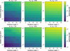 |
Fig. 4 Same as Fig. 3 but for H+ precipitation. |
| In the text | |
|
Fig. 5 N2 and N escape rates induced by magnetospheric N+ (upper panels) and H+ (lower panels) precipitation as functions of incident energy, ranging from 60-140 eV for N+ and 1-100 keV for H+. Results are shown for three scattering angle distributions corresponding to strong forward (αE = −1.5), isotropic (αE = 0.01), and backward (αE = 1.5) scattering conditions. |
| In the text | |
|
Fig. 6 Energy deposition and charge exchange rates for incident N+ under varying scattering parameter assumptions (αE = −1.5, −0.5, 0.01, 0.5, and 1.5, left column), incident energy (60-140 eV, middle column), and incidence angle (0°-80°, right column). The corresponding model parameters are indicated in each panel title. |
| In the text | |
|
Fig. 7 Same as Fig. 6 but for the energy deposition, charge exchange, and ionization rates driven by incident H+. |
| In the text | |
|
Fig. 8 Profiles of dissociation and ionization rates in Triton’s atmosphere resulting from the seven reactions studied in this work. Solid lines represent individual reaction contributions and the dashed line the total rate. All profiles result from an incident H+ population with an energy of 50 keV, an incidence angle of 55°, and a scattering parameter of –0.5. Red horizontal lines mark the altitudes corresponding to the peak densities of electron (solid, 330 km) and N+ (dashed, 460 km) for reference. |
| In the text | |
|
Fig. 9 Ionization rate profiles in Triton’s atmosphere induced by three energy sources: solar EUV radiation, magnetospheric electron precipitation, and magnetospheric ion precipitation. The black curve represents our simulation results for ion-driven ionization For comparison, ionization rates from previous studies are shown: solar EUV-driven (orange) and electron-driven (blue) ionization from Strobel et al. (1990a), and electron-driven ionization (green) from Benne et al. (2024). |
| In the text | |
|
Fig. B.1 Energy-dependent elastic, charge exchange, dissociation and ionization cross sections considered in this study. In panel (a), analytical fits for H+/H-N2 elastic cross sections, based on the semi-empirical formula of Lewkow et al. (2012), are shown as dashed lines. |
| In the text | |
Current usage metrics show cumulative count of Article Views (full-text article views including HTML views, PDF and ePub downloads, according to the available data) and Abstracts Views on Vision4Press platform.
Data correspond to usage on the plateform after 2015. The current usage metrics is available 48-96 hours after online publication and is updated daily on week days.
Initial download of the metrics may take a while.