| Issue |
A&A
Volume 702, October 2025
|
|
|---|---|---|
| Article Number | A237 | |
| Number of page(s) | 7 | |
| Section | Galactic structure, stellar clusters and populations | |
| DOI | https://doi.org/10.1051/0004-6361/202556420 | |
| Published online | 28 October 2025 | |
The X-ray luminosity function of stars observed with SRG/eROSITA
1
INAF – Osservatorio Astronomico di Brera,
Via E. Bianchi 46,
23807
Merate (LC),
Italy
2
Max-Planck-Institut für extraterrestrische Physik,
Gießenbachstraße 1,
85748
Garching bei München,
Germany
3
Como Lake Center for Astrophysics (CLAP), DiSAT, Università degli Studi dell’Insubria,
via Valleggio 11,
22100
Como,
Italy
4
Institut für Astronomie & Astrophysik, Eberhard Karls Universität Tübingen,
Sand 1,
72076
Tübingen,
Germany
★ Corresponding author: This email address is being protected from spambots. You need JavaScript enabled to view it.
Received:
15
July
2025
Accepted:
24
September
2025
Abstract
Background diffuse X-ray emission is contributed in large part by the emission of point sources that are not individually resolved. While this has been established for decades regarding the contribution of quasars to the diffuse emission above 1 keV energies, the possible contribution of undetected stars in the Milky Way to the softer band background emission (0.5−1 keV) is still poorly constrained. The overall unresolved X-ray flux from the stars is the product of the stellar spatial distribution in the Milky Way and the underlying X-ray luminosity function (XLF). In this work we determined the XLF of the stars and studied its structure with respect to a set of main-sequence spectral types (F, G, K, and M) and evolutionary stages (giants and white dwarfs). We built the XLF in volume-limited subsamples of increasing maximum distance and corresponding minimum X-ray luminosity using the HamStar catalog of X-ray-emitting stars detected in the western Galactic hemisphere with the extended ROentgen Survey with an Imaging Telescope Array (eROSITA) on board the Spectrum-Roentgen-Gamma (SRG) space observatory. We built an extinction-corrected Gaia color-magnitude diagram and decomposed the XLF into the relative contribution of different groups of stars. We provide an empirical polynomial description of the XLF for the total sample and for the different stellar subgroups that can be used to estimate the unresolved contribution from the stars to the soft X-ray background of the Milky Way in a flux-limited survey.
Key words: stars: luminosity function, mass function / X-rays: stars
© The Authors 2025
 Open Access article, published by EDP Sciences, under the terms of the Creative Commons Attribution License (https://creativecommons.org/licenses/by/4.0), which permits unrestricted use, distribution, and reproduction in any medium, provided the original work is properly cited.
This article is published in open access under the Subscribe to Open model. This email address is being protected from spambots. You need JavaScript enabled to view it. to support open access publication.
1 Introduction
Knowledge of the number density of a given class of astrophysical sources as a function of their luminosity is an essential tool for building forward models of the population in simulations (e.g., Belczynski et al. 2004; Belczynski & Taam 2004) and estimating the potential contribution of point sources of a given type to the unresolved background flux in shallow observations (e.g., Miyaji et al. 2000; Strong 2007; Revnivtsev et al. 2009). Estimates of the typical luminosity of a population must rely on volume-complete samples, that is, samples that collect information on all the sources within a given distance. In practice, real instrumentation characterized by a minimum detectable flux (Fmin) is unable to detect the faintest sources (put simply, F < Fmin). A best-case scenario is one in which the volume explored with a real instrument does not miss any source because the population within a distance maximum (dmax) is characterized by a physical luminosity  . However, in most cases, either the volume encompassed by the whole population is too large or the minimum detectable flux (Fmin) is too large, preventing us from detecting all the sources of the population. The practical solution that is eventually always implemented in real surveys is to reduce the size of the explored volume or study only the subset of the population more luminous than a minimum luminosity,
  .
.
So far, the only available volume-complete census for M dwarfs and FGK stars in X-rays has been limited to the closest 10–20 pc (Caramazza et al. 2023; Zhu & Preibisch 2025). A limitation of using small volumes is that they may be biased toward a subsample of the overall population. The small volume sample can, in fact, introduce a bias with respect to a given property (e.g., spectral type, age, and metallicity) simply because of the relatively small number of sources. If we were able to observe the whole Galactic volume, the average properties of the Galaxy (e.g., the luminosity of a given spectral type) would be computed correctly by definition, but this is currently not a realistic scenario.
X-ray emission from stars arises from magnetically confined hot plasma in the stellar corona, typically heated by magnetic reconnection (Güdel 2004). A proxy for the X-ray activity of stars is the X-ray-to-bolometric luminosity ratio, LX/Lbol. This quantity is a normalized measure of coronal activity, allowing a comparison of activity levels across stars regardless of size or spectral type. It is especially useful for tracing stellar evolution, activity saturation, and age-related trends. This is due to the dependence of the X-ray luminosity (LX) of a star on its fundamental properties, such as stellar radius, effective temperature, bolometric luminosity (Lbol), and mass. Therefore, LX/Lbol shows the level of intrinsic X-ray activity of the source, which is useful for studying the mechanism that produces the X-rays, for example by studying the dependence of LX/Lbol on age or rotation (e.g., Schmitt & Liefke 2004; Preibisch & Feigelson 2005; Kiraga & Stepien 2007; Donati et al. 2008; Johnstone & Güdel 2015; Wright et al. 2018; Pizzocaro et al. 2019; Magaudda et al. 2020; Johnstone et al. 2021; Magaudda et al. 2022; Stelzer et al. 2022).
In this work, we aim to extend our knowledge on the X-ray luminosities of stars to larger volumes by computing the X-ray luminosity function (XLF) for X-ray subsamples defined by LX > LX,min within a maximum given distance dmax(LX,min). Effectively, we hereby extend the volume limit to distances much beyond 10 pc. We also focus on the XLF of the LX luminosity, as we want to determine how much X-ray emission overall is going to be produced by a given kiloparsec-scale portion of the Milky Way disk. By building large samples that minimize the sensitivity selection bias, we averaged over the details of particular stellar populations and types and provide a weighted average luminosity that can be used to estimate the overall X-ray background from unresolved stars. The exact computation of this background would require building a forward model of the solar neighborhood that assigns the (un)known correct luminosity function to field stars and to every stellar cluster and association at the corresponding 3D location. However, the knowledge required to build such a fundamentally important forward model is neither complete nor available. The approach of this work thus provides a very useful tool for approximating the overall stellar X-ray output from wide regions of the Milky Way by computing it over large samples. In other words, we do not focus on a specific stellar property and instead encompass all possible physical mechanisms that produce X-rays from stars with their observed relative fractions in order to provide a description of the total X-ray output.
2 Data
The HamStar catalog (Freund et al. 2024) provides information on all point sources identified as coronally active stars detected in the first extended ROentgen Survey with an Imaging Telescope Array (eROSITA) all-sky survey (eRASS1; Merloni et al. 2024) of the western Galactic hemisphere. The catalog reports FX fluxes in the soft X-ray band (0.2–2.3 keV). Relevant information provided for each entry in the catalog is the best-matched Gaia Data Release 3 (DR3) counterpart (Gaia Collaboration 2021) and, thus, the Gaia distance, color (Bp – Rp), and G band magnitude (G). We note that the HamStar magnitudes and colors are not corrected for extinction. We used the available extinction information (AGSP,g; EGSP(Bp – Rp)) from the Gaia GSP-Phot Aeneas library1. This library uses a Bayesian framework to estimate stellar parameters from low-resolution spectra (Bailer-Jones 2011) and is currently being implemented into the Gaia data processing pipeline. We used the available information to compute corrected G-band magnitudes, g0 = g − AGSP,g (then converted them to the absolute magnitude, G0) and colors, (Bp− Rp)0 = (Bp − Rp) − EGSP(Bp − Rp). The Gaia information thus allowed us to build a color-magnitude diagram (G0; (Bp − Rp)0) and to divide the sample by spectral type. In addition, by combining the X-ray flux (FX) with the Gaia distance, we can compute the X-ray luminosity (LX) for all the stars from the HamStar catalog.
3 Method
The HamStar catalog is a flux-limited sample of X-ray-emitting stars. An additional selection is thus necessary in order to build a volume-limited sample for computing the XLF. To build such subsamples, we chose a set of maximum distances, {dmax,i} Within a given (increasing) dmax,i, we selected all the stars with an X-ray luminosity higher than  . Each subsample is then volume-limited by construction for stars above the LX,min threshold, defined by the subsample’s maximum distance, dmax,i.
As the flux limit we used Fmin = 5 × 10⁻¹⁴ erg s−1 cm−2. This value is the most frequent flux bin in the HamStar catalog and is the eRASS1 equatorial detection threshold estimated by Predehl et al. 2021. It is also similar to the value found by Magaudda et al. (2022) of Fmin ~ 3 × 10⁻¹⁴ erg s−1 cm−2 for a sample of ~ 700 M dwarfs within 150 pc.
Figure 1 shows these subsamples (the same color code is used in all figures in this work) plotted on top of the whole HamStar sample. The stars matching our selection criteria show a homogeneous distribution within each 3D spherical volume, with minor concentrations in the location of neighboring clusters (see Appendix A).
To identify the spectral type of the stars in our sample, we built the color-magnitude diagram (G0; (Bp − Rp)0) shown in Fig. 2. The subscript 0 indicates that the values have been corrected for extinction, which we did when GSP-Phot extinction values were available in the Gaia DR3 database (74% of our sample). When the GSP-Phot extinction values were not available (26% of our sample), we did not compute the correction and used the values as originally reported in HamStar. We defined the main-sequence spectral types F, G, K, and M using the Gaia-corrected colors, according to the online table of Eric Mamajek2. We assigned all giant and supergiant stars to one group regard-less of their color. The threshold line between main-sequence stars and giants is defined here as G0 ≡ 3.7 ⋅ (1 + log10(Bp−Rp)0) for (Bp − Rp)0 < 1.84, and G0 < 6 for (Bp − Rp)0 > 1.84. While not based on a physical motivation, this definition effectively separates the bulk of FGK main-sequence stars from giant branch stars with similar (Bp − Rp)0 Gaia colors. A similar approach was taken to separate the white dwarfs (WDs), and main-sequence stars of spectral type earlier than F. The latter, in particular spectral types A and B, are usually characterized by radiative envelopes, where magnetic dynamo action is suppressed due to the lack of convection in the stellar envelope. The X-ray emission from these systems is thus most likely associated with an unresolved companion star (e.g., Stelzer et al. 2006). We therefore named this set “late-type companion?”. While giant stars are X-ray emitters, they are characterized in general by a slower rotation in their late evolutionary phase and, thus, likely have a less efficient dynamo than main-sequence stars. Therefore, some of their X-ray flux may also be produced by a companion star. A detailed characterization of each of these sources is beyond the scope of this work, and thus we relied on the HamStar identification of the Gaia giant star counterparts. The WD subsample also includes binary systems with a main-sequence companion star. The sample is defined by G0 > 3.5 ⋅ (Bp − Rp )0 + 3.1 for (Bp − Rp)0 < 1.84 (i.e., earlier colors than M dwarfs). The division of the subsamples is illustrated in Fig. 2 with dashed lines. Based on the large statistics available thanks to the large volumes, we verified that different definitions for the thresholds close to the one provided above do not produce significant changes in the derived XLF.
We also note that the median of the relative correction to the color is only 10–12% across all spectral types. Therefore, the lack of extinction values for 26% of our sample does not introduce a significant bias in the separation of the spectral types.
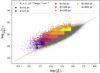 |
Fig. 1 X-ray luminosity-distance phase space of the distance-limited samples (colors) and of the full HamStar catalog (gray points). The same color code is used in the other figures in this paper. |
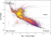 |
Fig. 2 Gaia DR3 color-magnitude diagram of the HamStar catalog (gray points). |
4 Results
In Fig. 3, we show the XLF derived with our method including all the stars, regardless of their group in the color-magnitude diagram. The XLF of each subsample defined by a given Lmin,i is shown with its corresponding color. The XLF data points of adjacent subsamples (i.e., different Lmin,i) overlap within each of the shared luminosity bins. Smaller volumes miss rare high-luminosity stars, while larger volumes miss low-luminosity bins due to higher Lmin,i thresholds. Altogether, they produce a smooth XLF extended over the LX ∈ [2.5 × 1027; 7.5 × 1031] erg s−1 range.
Following the same procedure, we computed the XLF for all the groups defined in Fig. 2. The result is shown in Fig. 4. We also derived the XLF from the 10 pc sample of Caramazza et al. 2023 (cyan star markers). Their volume-limited sample involved dedicated XMM-Newton follow-up. Therefore, it extends to lower X-ray luminosities with respect to the eROSITA-based HamStar catalog. In their work, most of the M dwarf stars within 10 pc of the Sun have been detected in X-rays (144 of 149 stars). The XLF data points derived in this work for the M dwarf sample (blue dots) overlap with the XLF derived from the 10 pc sample in the higher-LX bins, confirming that our XLF is a good approximation to a volume-complete result within eROSITA’s sensitivity range. We also note that the highest-luminosity bins of the 10 pc sample have relatively large statistical uncertainties and scatter compared to the same bins of our M dwarf sample (blue points). This statistical improvement is due to the approach of separating volume-limited samples of increasing luminosity and distance generally providing larger samples.
In this paper, we focus on the XLFs derived for the main-sequence spectral types F, G, K, and M, while also reporting the results for the other stellar groups defined by our color-magnitude diagram for completeness. We note that the spectral type assigned to sources labeled “late-type companion?” may have more contamination from possible companion stars than those classified as F, G, K, or M types. However, as their X-ray emission still meets our flux–distance selection criteria, we included them in the computation of the overall XLF. An additional test on true binary systems resolved by both Gaia (El-Badry et al. 2021) and eROSITA (separation > 10″) yields an XLF consistent within 5% with that derived from the whole sample (see Appendix B for details).
We find that M dwarfs dominate the low-luminosity end of the XLF, LX < 1029 erg s−1.F-, G-, and K-type stars dominate in the 1029 − 5 × 1030 erg s−1 luminosity range, while at higher luminosities giant and supergiant stars are the most frequent X-ray-emitting stellar group (their XLF is poorly constrained below 1029 erg s−1).
We performed polynomial fits for each of the XLFs. The coefficients are reported in Table 1. We fixed the number of coefficients to 4, which we found to be the lowest degree that can provide a reasonable fit for all stellar groups. The fitted polynomials are shown in Fig. 4.
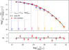 |
Fig. 3 XLF of the stars in our sample (all). The vertical dotted lines show the minimum luminosity corresponding to the maximum distance in parsecs (label) of each subset. |
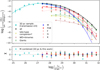 |
Fig. 4 XLF of stars in different parts of the color-magnitude diagram. The different colors show the contribution of the different stellar groups to the total XLF, as labeled. The red star symbols of Fig. 3, corresponding to the XLF values for all groups combined, are shown as the black points. |
Coefficients of the polynomial fit XLFSpT = Σn an(log LX)n.
5 Discussion
Knowledge of the low-luminosity end of the XLF is restricted to the closest regions of the solar neighborhood due to instrumental flux limits. A complete census of all stellar X-ray emitters even in the smallest volume around the Sun requires dedicated XMM-Newton observations. This was achieved by the 10 pc survey described by Caramazza et al. (2023). We find that the XLF derived in our work from eRASS1 matches that derived from the volume-complete 10 pc M dwarf sample in the common range of luminosities analyzed. We note that the Caramazza et al. 2023 survey comprises only M dwarf stars of subtypes M0-M4. However, we find that subtypes M0-M4 account for >96% of the stars in the eRASS1 M dwarf sample, making a further selection for the comparison unnecessary.
Figure 4 shows that the high-luminosity tail of the XLF is missing from the 10 pc sample, as small volumes necessarily lack information on rare objects, such as those at the high-luminosity tail of the XLF. This implies that the average X-ray luminosity value, 〈LX〉, from the 10 pc sample is biased low with respect to the overall galactic M dwarf population. We define the bias as 1 − C10pc/CM − where the latter element is the ratio between the integral  derived from the 10 pc sample and that computed in this work for M dwarfs – and define L0 = 1027 erg s−1 as the sensitivity limit of eRASS1 for M dwarfs according to the HamStar catalog (Freund et al. 2024). We obtain a bias of 2%. Given that our lower integration boundary, L0, is higher than the minimum luminosity reached by the 10 pc sample, the value of 2% is actually an upper limit to the true bias. By joining the M dwarf XLF derived in this work with that derived for the 10 pc sample, and setting L0 = 1024 erg s−1, we obtain a bias of only 0.3%.
To determine which luminosities are represented in which volumes for a given spectral type, we plotted (see the upper panel of Fig. 5) the X-ray luminosity (LX) versus the Gaia color (Bp − Rp; extinction-corrected when possible) for all the stars in our sample (i.e., we included late-type companions and WD+binaries groups) except the group of giants (see Appendix C for the giant stars). In general, the number of stars increases in larger volumes until a certain value for the maximum distance (e.g., dmax,i = 800 pc for main-sequence F, G, and K stars), where the corresponding luminosity threshold (e.g., Lmin,i = 5.4 × 1030 erg s−1 for dmax,i = 800 pc) is high enough to strongly limit the number of available sources. Almost no M dwarfs were selected within the largest volumes. This fact is consistent with the general maximum luminosity of M dwarfs of a few times 1030 erg s−1 (Magaudda et al. 2020, 2022). F, G, and K stars, however, reach higher X-ray luminosities and can thus be detected from greater distances.
In the lower panel of Fig. 5 we show a similar plot that considers the level of X-ray activity defined as LX/Lbol (see Appendix E for details on the bolometric luminosity, Lbol). The range in X-ray activity spans about 3 dex for each group (F, G, K, and M), but for successively higher values. This plot clearly shows that our definition of the subsamples necessarily introduces a selection bias with respect to the X-ray activity. In fact, the continuous decrease in Lbol toward later spectral types limits the LX/Lbol value of M dwarfs to larger values, as shown by the positive trend in the lower panel of Fig. 5. This selection bias prevents an unbiased assessment of the LX/Lbol distribution of our sample. While its correct computation could be obtained via forward-modeling as a function of the other parameters (LX and spectral type), this approach is still limited by the available volume-limited samples (Zhu & Preibisch 2025). A forward modeling of the LX/Lbol distribution thus goes well beyond the data-driven approach of this work.
An additional potential source of bias in the derived stellar density per luminosity bin, nd log L, may be introduced by a 3D disk-like spatial distribution of sources, compared to a homogeneous distribution. In fact, according to the definition  , the source distribution is assumed to be homogeneous over a spherical volume. The bias becomes important for dmax ≫ zh, where zh is the disk scale-height. The thin and thick disks of the Milky Way have values of ≃300 and 900 pc, respectively (Jurić et al. 2008; McMillan 2017). The bias is thus only potentially affecting our largest volume-luminosity bin, where M dwarfs are in practice not represented. This affects only a single data point in our derivation of the XLF (see Appendix D). Deeper surveys (dmax ≥ 1 kpc) should, however, take this bias into consideration.
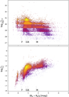 |
Fig. 5 Upper panel: luminosity–color phase space of all the stars in our sample (apart from the giant group; for those, see Appendix C). Lower panel: X-ray fractional luminosity versus Gaia color. Sources without available bolometric correction were not displayed. |
6 Conclusion
Using eRASS1 data and its stellar identification from the Ham-Star catalog (Freund et al. 2024), we have computed the XLF of stars per stellar group, probing distances of up to 800 pc from the Sun. We find that for the eRASS1 sensitivity limit Flim = 5 × 10¹⁴ erg s−1 cm−2, M dwarfs, FGK-type stars, and giants dominate the XLF above LX ~ 1027, 1029, and 5 × 1030 erg s−1, respectively. The previously known XLF of M dwarfs probes the closest 10 pc to the Sun (Caramazza et al. 2023; Zhu & Preibisch 2025). The comparison with our sample shows that the volume-complete (10 pc) approach probes the lowest X-ray luminosities for this spectral type, which are only accessible in the smallest volumes, but it misses the rare high-luminosity stars. The XLF derived in this work is able to both probe the high-luminosity end and explore the XLF over the largest volume to date for sufficiently high X-ray luminosities, both for M dwarfs and other spectral types. We provide polynomial fits for the XLF of all stellar groups, including main-sequence stars (F, G, K, and M), giants, and WD+binaries. The results from our polynomial fits to the XLF can be used to model the X-ray stellar contribution to the unresolved soft X-ray emission of Milky Way-like galaxies. Improved knowledge on both ends of the XLF (and of the X-ray activity) can only come from future all-sky surveys reaching lower X-ray fluxes than eROSITA or from complete surveys, which are feasible only for very small sky volumes.
Acknowledgements
We acknowledge financial support from the European Research Council (ERC) under the European Union’s Horizon 2020 research and innovation program Hot-Milk (grant agreement No. 865637). GP acknowledges support from Bando per il Finanziamento della Ricerca Fondamentale 2022 dell’Istituto Nazionale di Astrofisica (INAF): GO Large program and from the Framework per l’Attrazione e il Rafforzamento delle Eccellenze (FARE) per la ricerca in Italia (R20L5S39T9). E.M. was supported by Deutsche Forschungs-gemeinschaft under grant STE 1068/8-1. We thank the anonymous reviewer for helping to improve the manuscript.
Appendix A 3D spatial distribution
In Figs. A.1 and A.2 we plot the location of the stars in our sample, in 2D projections around the Sun as seen from far above (XY) and within (XZ) the Milky Way mid-plane, respectively. Given the broad range of scales in distances of the different sub-samples, the right half of the plots zooms in the closest 200 pc to the Sun to highlight the position of the closest stars, i.e., as the HamStar sample only explores the western Galactic sky based on the data available to the German eROSITA Consortium, the right-hand part of the figures has a mirrored X-axis. It can be seen that the stars are mostly homogeneously distributed within each 3D spherical volume. It is also possible to identify clusters of stars. Given the relative size and population of these overdensities, we conclude that our selection is not strongly biased toward a particular direction in the sky.
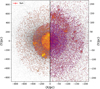 |
Fig. A.1 X-Y projection of the position of the HamStar catalog (gray points). The selection of the volume-limited subsamples is shown. The right half of the plot shows a zoomed-in view of the nearest 200 pc to the Sun with a mirrored X coordinate. |
Appendix B Multiplicity
Given the higher spatial resolution of the Gaia DR3 data compared to eROSITA (~1.5 and 10 arcsec, respectively), several optical counterparts for a given X-ray source are often found in the positional cross-match. This issue is already discussed in detail in the HamStar description (Freund et al. 2024) for the interested reader. While we do not repeat the cross-matches, we verify that our XLF is not influenced by the selection of the wrong optical counterpart in binary systems. To this end, we consider a subsample of the one used in this work that includes all and only the stars recognized as part of a binary system with angular separation ∆θ between the companion stars i.e., larger than the eROSITA resolution of 10 arcsec). This is possible thanks to the catalog of Gaia binary systems El-Badry et al. (2021). This catalog is based on the Gaia DR3 sources and is cleaned from chance positional coincidence of stars 3. By selecting ∆θ > 10 arcsec, we obtain only stars that are known to have a companion, but the companion can be resolved with eROSITA.
From the cross-match with the catalog by El-Badry et al. (2021), we find that ~22% of the whole sample used in this work is part of binary systems with ∆θ > 10 arcsec. The XLFs built on this additional selection (binaries with ∆θ > 10 arcsec, cyan and orange squares in Fig. B.1 for the M and FGK groups, respectively) match the XLFs of the original group samples (blue and red squares for the M and FGK groups, respectively) always within 5% for all luminosity bins. This result shows that our derivation of the XLF is relatively robust against spurious cross-match due to multiplicity.
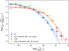 |
Fig. B.1 Comparison between the XLF for the subsample of members of binary systems with ∆θ > 10 arcsec (red squares) and the XLF derived from the whole sample used in this work (black dots, equal to Fig. 4). |
Appendix C Giant stars
In Fig. C.1 we show equivalents of the upper and lower panels of Fig. 5 (left and right panel, respectively), for the giants group. We note that most of the giants show very high X-ray luminosity that are statistically more likely to be found in the largest volumes given the relatively low frequency. We note that most of the population of M-type giant stars may be missing, although they are the majority of all giants according to stellar models.
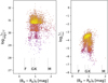 |
Fig. C.1 Left panel: X-ray luminosity–color phase space of the distance subsamples for the giant star group. Right panel: X-ray activity-color for the same samples. |
Appendix D Exponential versus homogeneous height distribution
We verified numerically that for a known XLF, the one derived applying our selection criteria is not affected for the values of dmax reached in this work whether assuming a homogeneous or disk-like distribution of sources. To this end, for simplicity we assume a power-law XLF with low- and high- luminosity cut-offs. We generate X-ray sources at random locations (X, Y, Z) around the Sun where X and Y lay on the Galactic mid-plane and Z is the height above the plane. We draw X, Y and Z from uniform probability distribution functions. The X-ray luminosity of each source is randomly drawn from the assumed power-law XLF. We then apply our selection criteria of LX > LX,min& d < dmax(LX,min) to the mock sample. The number of simulated sources is chosen in order to match (after selection) the number of sources of the observed sample. We check that the XLF derived from this mock sample reproduces the assumed one in all luminosity bins within the statistical uncertainties.
We then repeated the simulation by only varying the probability distribution of the Z coordinate PDF(Z) in order to test a different distribution of the stars with height from the Galactic plane. This time we draw the Z coordinate from the function PDF(Z)  . The X and Y coordinates and the X-ray luminosities are drawn again, in the same way as in the simulation for homogeneous spherical distribution, outlined above. The result is shown in Fig. D.1. The computed XLF (the red squares are the median values in each luminosity bin) are fitted with a power-law model (cyan dashed line) which is in good agreement with the assumed XLF (blue solid line) within the statistical uncertainties for all values of Zh ≤ 400 pc. This is due to the fact that for Z < Zh, PDF(z) → const, so that we fall again in the homo-geneous scenario. The values shown by the yellow squares are high-luminosity sources in the largest volume. They are possibly biased low due to the thin disk geometrical effect, as shown by the slightly lower fit values (cyan dashed line) compared to the assumed XLF (blue solid line) in these bins. However, the real case scenario is composed by the sum of a thin (Zh ≃ 300 pc) and a thick disk (Zh ≃ 900 pc). The additional presence of a thick disk thus smooths this biases further compared to our simulation. The total bias is thus negligible for the distance values considered in this work.
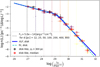 |
Fig. D.1 Simulated XLF from a disk-like distribution of sources. |
Appendix E Bolometric luminosity, Lbol,
The bolometric luminosity Lbol is computed through the standard set of equations:
 (E.1)
(E.1)
 (E.2)
(E.2)
where Mbol,⊙ = 4.66 is the absolute bolometric magnitude of the Sun, as calibrated by Gaia (Creevey et al. 2023) to estimate the bolometric correction BCG to the G band extinction-corrected absolute magnitude G0. The bolometric correction BCG is tabulated in the bc_flame parameter columns of the Gaia DR3 astrophysical_parameter table4. The bc_flame value is a function of effective temperature, surface gravity, and metallicity, and has been derived from MARCS synthetic stellar spectra library (Gustafsson et al. 2008) applied to the GSP-Photometry results on the Gaia DR3 sources. We note that these are the same Gaia DR3 entries for which extinction correction information was computed. The bolometric luminosity of the Sun is Lbol,⊙ = 3.828 × 1033erg s−1.
References
- Bailer-Jones, C. A. L. 2011, MNRAS, 411, 435 [Google Scholar]
- Belczynski, K., & Taam, R. E. 2004, ApJ, 603, 690 [NASA ADS] [CrossRef] [Google Scholar]
- Belczynski, K., Kalogera, V., Zezas, A., & Fabbiano, G. 2004, ApJ, 601, L147 [NASA ADS] [CrossRef] [Google Scholar]
- Caramazza, M., Stelzer, B., Magaudda, E., et al. 2023, A&A, 676, A14 [NASA ADS] [CrossRef] [EDP Sciences] [Google Scholar]
- Creevey, O. L., Sordo, R., Pailler, F., et al. 2023, A&A, 674, A26 [NASA ADS] [CrossRef] [EDP Sciences] [Google Scholar]
- Donati, J. F., Morin, J., Petit, P., et al. 2008, MNRAS, 390, 545 [Google Scholar]
- El-Badry, K., Rix, H.-W., & Heintz, T. M. 2021, MNRAS, 506, 2269 [NASA ADS] [CrossRef] [Google Scholar]
- Freund, S., Czesla, S., Predehl, P., et al. 2024, A&A, 684, A121 [NASA ADS] [CrossRef] [EDP Sciences] [Google Scholar]
- Gaia Collaboration (Brown, A. G. A., et al.) 2021, A&A, 649, A1 [NASA ADS] [CrossRef] [EDP Sciences] [Google Scholar]
- Güdel, M. 2004, A&A Rev., 12, 71 [Google Scholar]
- Gustafsson, B., Edvardsson, B., Eriksson, K., et al. 2008, A&A, 486, 951 [NASA ADS] [CrossRef] [EDP Sciences] [Google Scholar]
- Johnstone, C. P., & Güdel, M. 2015, A&A, 578, A129 [NASA ADS] [CrossRef] [EDP Sciences] [Google Scholar]
- Johnstone, C. P., Bartel, M., & Güdel, M. 2021, A&A, 649, A96 [EDP Sciences] [Google Scholar]
- Juric, M., Ivezic, Ž., Brooks, A., et al. 2008, ApJ, 673, 864 [NASA ADS] [CrossRef] [Google Scholar]
- Kiraga, M., & Stepien, K. 2007, Acta Astron., 57, 149 [NASA ADS] [Google Scholar]
- Magaudda, E., Stelzer, B., Covey, K. R., et al. 2020, A&A, 638, A20 [NASA ADS] [CrossRef] [EDP Sciences] [Google Scholar]
- Magaudda, E., Stelzer, B., Raetz, S., et al. 2022, A&A, 661, A29 [NASA ADS] [CrossRef] [EDP Sciences] [Google Scholar]
- McMillan, P. J. 2017, MNRAS, 465, 76 [NASA ADS] [CrossRef] [Google Scholar]
- Merloni, A., Lamer, G., Liu, T., et al. 2024, A&A, 682, A34 [NASA ADS] [CrossRef] [EDP Sciences] [Google Scholar]
- Miyaji, T., Hasinger, G., & Schmidt, M. 2000, A&A, 353, 25 [NASA ADS] [Google Scholar]
- Pizzocaro, D., Stelzer, B., Poretti, E., et al. 2019, A&A, 628, A41 [NASA ADS] [CrossRef] [EDP Sciences] [Google Scholar]
- Predehl, P., Andritschke, R., Arefiev, V., et al. 2021, A&A, 647, A1 [EDP Sciences] [Google Scholar]
- Preibisch, T., & Feigelson, E. D. 2005, ApJS, 160, 390 [NASA ADS] [CrossRef] [Google Scholar]
- Revnivtsev, M., Sazonov, S., Churazov, E., et al. 2009, Nature, 458, 1142 [Google Scholar]
- Schmitt, J. H. M. M., & Liefke, C. 2004, A&A, 417, 651 [NASA ADS] [CrossRef] [EDP Sciences] [Google Scholar]
- Stelzer, B., Huélamo, N., Micela, G., & Hubrig, S. 2006, A&A, 452, 1001 [NASA ADS] [CrossRef] [EDP Sciences] [Google Scholar]
- Stelzer, B., Klutsch, A., Coffaro, M., Magaudda, E., & Salvato, M. 2022, A&A, 661, A44 [NASA ADS] [CrossRef] [EDP Sciences] [Google Scholar]
- Strong, A. W. 2007, Ap&SS, 309, 35 [Google Scholar]
- Wright, N. J., Newton, E. R., Williams, P. K. G., Drake, J. J., & Yadav, R. K. 2018, MNRAS, 479, 2351 [Google Scholar]
- Zhu, E., & Preibisch, T. 2025, A&A, 694, A93 [NASA ADS] [CrossRef] [EDP Sciences] [Google Scholar]
“A Modern Mean Dwarf Stellar Color and Effective Temperature Sequence” – http://www.pas.rochester.edu//~emamajek/EEM_dwarf_UBVIJHK_colors_Teff.txt – version 2022.04.16.
For all the Gaia stars it is not possible to tell whether they hold or not a companion closer than the Gaia resolution of 1.5 arcsec and we know all the binaries resolved by Gaia but not by eROSITA (1.5 > ∆θ > 10 arcsec).
All Tables
All Figures
|
Fig. 1 X-ray luminosity-distance phase space of the distance-limited samples (colors) and of the full HamStar catalog (gray points). The same color code is used in the other figures in this paper. |
| In the text | |
|
Fig. 2 Gaia DR3 color-magnitude diagram of the HamStar catalog (gray points). |
| In the text | |
|
Fig. 3 XLF of the stars in our sample (all). The vertical dotted lines show the minimum luminosity corresponding to the maximum distance in parsecs (label) of each subset. |
| In the text | |
|
Fig. 4 XLF of stars in different parts of the color-magnitude diagram. The different colors show the contribution of the different stellar groups to the total XLF, as labeled. The red star symbols of Fig. 3, corresponding to the XLF values for all groups combined, are shown as the black points. |
| In the text | |
|
Fig. 5 Upper panel: luminosity–color phase space of all the stars in our sample (apart from the giant group; for those, see Appendix C). Lower panel: X-ray fractional luminosity versus Gaia color. Sources without available bolometric correction were not displayed. |
| In the text | |
|
Fig. A.1 X-Y projection of the position of the HamStar catalog (gray points). The selection of the volume-limited subsamples is shown. The right half of the plot shows a zoomed-in view of the nearest 200 pc to the Sun with a mirrored X coordinate. |
| In the text | |
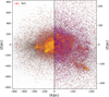 |
Fig. A.2 Same as Fig. A.1 but for the X-Z projection. |
| In the text | |
|
Fig. B.1 Comparison between the XLF for the subsample of members of binary systems with ∆θ > 10 arcsec (red squares) and the XLF derived from the whole sample used in this work (black dots, equal to Fig. 4). |
| In the text | |
|
Fig. C.1 Left panel: X-ray luminosity–color phase space of the distance subsamples for the giant star group. Right panel: X-ray activity-color for the same samples. |
| In the text | |
|
Fig. D.1 Simulated XLF from a disk-like distribution of sources. |
| In the text | |
Current usage metrics show cumulative count of Article Views (full-text article views including HTML views, PDF and ePub downloads, according to the available data) and Abstracts Views on Vision4Press platform.
Data correspond to usage on the plateform after 2015. The current usage metrics is available 48-96 hours after online publication and is updated daily on week days.
Initial download of the metrics may take a while.