| Issue |
A&A
Volume 702, October 2025
|
|
|---|---|---|
| Article Number | A256 | |
| Number of page(s) | 6 | |
| Section | Stellar structure and evolution | |
| DOI | https://doi.org/10.1051/0004-6361/202556620 | |
| Published online | 28 October 2025 | |
Studying the black widow pulsars PSR J0312–0921 and PSR J1627+3219 in the optical and X-rays
1
Ioffe Institute, 26 Politekhnicheskaya, St., Petersburg, 194021, Russia
2
Instituto de Astronomía, Universidad Nacional Autónoma de México, Apdo. Postal 877, Ensenada, Baja California, 22800, Mexico
3
American Association of Variable Star Observers, 185 Alewife Brook Parkway, Suite 410, Cambridge, MA 02138, USA
⋆ Corresponding author: This email address is being protected from spambots. You need JavaScript enabled to view it.
Received:
28
July
2025
Accepted:
27
August
2025
Abstract
Context. PSR J0312−0921 and PSR J1627+3219 are black widow pulsars with orbital periods of 2.34 and 3.98 hours. They were recently detected in the radio and γ-rays.
Aims. Our goals were to estimate the fundamental parameters of both binary systems and their components.
Methods. We performed first phase-resolved multi-band photometry of both objects with the 10.4 m Gran Telescopio Canarias and fitted the obtained light curves with a model assuming direct heating of the companion by the pulsar. Archival X-ray data obtained with the Swift and XMM-Newton observatories were also analysed.
Results. For the first time, we firmly identified both systems in the optical. Their optical light curves show a rather symmetric single peak per orbital period and a peak-to-peak amplitude of ≳2 mag. We also identified the X-ray counterpart to J1627+3219, and for J0312−0921 we set an upper limit on the X-ray flux.
Conclusions. We estimated the masses of the pulsars, companion temperatures and masses, Roche lobe filling factors, orbital inclinations, and the distances to both systems. PSR J0312−0921 has a very light companion (≈0.02 M⊙) that possibly has one of the lowest night-side temperatures of the known black widow systems (≈1600 K). We find that the distances to J0312−0921 and J1627+3219 are about 2.5 and 4.6 kpc, respectively. This likely explains their faintness in X-rays. The X-ray spectrum of PSR J1627+3219 can be described by a power-law model, and its parameters are compatible with those obtained for other black widows.
Key words: binaries: general / stars: neutron
© The Authors 2025
 Open Access article, published by EDP Sciences, under the terms of the Creative Commons Attribution License (https://creativecommons.org/licenses/by/4.0), which permits unrestricted use, distribution, and reproduction in any medium, provided the original work is properly cited.
This article is published in open access under the Subscribe to Open model. This email address is being protected from spambots. You need JavaScript enabled to view it. to support open access publication.
1. Introduction
Black widows (BWs) form a subclass of the so-called spider systems, which are binary millisecond pulsars (MSPs) with short orbital periods (Pb ≲ 1 d) and low-mass companions (Mc ≲ 0.05 M⊙ for BWs; Roberts 2013). The companion in these systems is heated and evaporated by the pulsar high-energy radiation and the wind of relativistic particles, which can cause eclipses of the pulsar radio emission. BW pulsars are recycled via the accretion of matter and angular momentum from main-sequence companion stars during the low-mass X-ray binary stage (Bisnovatyi-Kogan & Komberg 1974; Alpar et al. 1982). In addition, BWs have been proposed as potential progenitors of isolated MSPs (e.g. Ginzburg & Quataert 2020; Guo et al. 2022). However, the formation pathway of such systems is not yet completely clear (Chen et al. 2013; Benvenuto et al. 2014; Ginzburg & Quataert 2021; Guo et al. 2024).
To date, 49 confirmed BWs have been discovered in the Galactic field, mainly through observations in the radio and γ-rays (Koljonen & Linares 2025). These observations can provide information on the source position, pulsar mass function, spin period, binary period, and distance. Optical studies of BW systems are crucial for obtaining other fundamental parameters such as the companion’s surface temperature distribution, Roche-lobe filling factor, and irradiation efficiency. Moreover, they are useful for measuring the masses of binary components, orbital inclinations, and distances, especially in cases where these parameters cannot be constrained well from radio or γ-ray timing observations alone. Recent optical studies of a sample of BWs provided valuable constraints on their system parameters (Draghis et al. 2019; Mata Sánchez et al. 2023; Bobakov et al. 2024).
The BW pulsars PSR J0312−0921 and PSR J1627+3219 (hereafter J0312 and J1627) were recently discovered with the Green Bank Telescope and the Five hundred meter Aperture Spherical radio Telescope, respectively, during searches for unassociated Fermi Large Area Telescope (LAT) γ-ray sources (Tabassum et al. 2021; Saz Parkinson 2021; Li et al. 2022). Pulsations with the pulsars’ spin periods were also detected in γ-rays (Smith et al. 2023). The parameters of the systems are presented in Table 1. We note that the J0312 orbital period, 2.34 h, is among the shortest of the known BWs (see e.g. Swihart et al. 2022).
J0312 and J1627 parameters.
Here we report the results of the first multi-band optical observations of J0312 and J1627 with the 10.4 m Gran Telescopio Canarias (GTC). In addition, we analysed archival X-ray observations carried out with the Swift X-Ray Telescope (XRT) and XMM-Newton observatory. The paper is organised as follows: Optical observations and data reduction are described in Sect. 2, and the modelling of the light curves in Sect. 3. Analysis of the X-ray data is presented in Sect. 4. Discussion and conclusions are given in Sect. 5.
2. Optical observations and data reduction
2.1. J0312
The phase-resolved photometric observations1 of the J0312 field were performed during two observing runs in October 2023 in the Sloan g′, r′, and i′ bands with the Optical System for Imaging and low Resolution Integrated Spectroscopy (OSIRIS+) instrument2. The OSIRIS+ field of view (FoV) is 7 8 × 7
8 × 7 8 with a pixel scale of 0
 254 in the standard 2 × 2 binning mode.
The observations were carried out under photometric weather conditions. To avoid effects from CCD defects, we used 5 dithering between the individual exposures. Each observing run (with durations of about 2.7 h and 2.3 h) covered approximately one orbital period of the system. To optimise the efficiency of observations, in the first run we used the alternating g′ and r′ bands, while in the second run the BW period was covered in the r′ and i′ bands. The log of observations is presented in Table 2 and the r′-band image of the pulsar field is shown in the top panel of Fig. 1, where the variability of the pulsar companion is demonstrated in the insets.
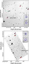 |
Fig. 1. Optical images of the fields of the two pulsars. Top panel: 3 |


Standard data reduction, including bias subtraction and flat-fielding, was performed using the Image Reduction and Analysis Facility (IRAF) package. We applied the L.A.Cosmic algorithm (van Dokkum 2001) to remove cosmic-ray events. For astrometric referencing, we used a single 180 s r′-band image and a set of stars from the Gaia Data Release 3 catalogue (Gaia Collaboration 2023). The formal rms uncertainties of the fit were Δα ≲ 0 13 and Δδ ≲ 0
 14.
14.
For the photometric calibration, we used the Sloan photometric standard SA 112-805 (Smith et al. 2002) observed during the same nights as the target. Accounting for the extinction coefficients kg′ = 0.15(2), kr′ = 0.07(1), and ki′ = 0.04(1) (Cabrera-Lavers et al. 2014), we calculated the zero points Zg′ = 28.07(2), Zr′ = 28.09(1) (2023 October 10), Zr′ = 28.02(1) (2023 October 11), and Zi′ = 27.58(1). We verified these zero points using a set of stars from the Panoramic Survey Telescope and Rapid Response System (Pan-STARRS) Data Release 2 (DR2) catalogue (Flewelling et al. 2020, see Fig. 1) and short exposures obtained in each band for the calibration purposes. The 3σ detection limits during the observations were g′≈26.5 mag, r′≈25.75 − 25.9 mag, and i′≈24.6 − 24.8 mag. We note that all magnitudes presented in this paper are in the AB system.
We used the optimal extraction algorithm (Naylor 1998), to extract the target light curves and applied a differential technique to eliminate the variations due to the changing weather conditions using a non-variable bright field star from the Pan-STARRS DR2 catalogue as a reference (Fig. 1, top). Its magnitude scatters were ≲0.05 mag during the runs.
2.2. J1627
The phase-resolved multi-band observations of the J1627 field were performed on 2024 July 293 with the HiPERCAM instrument4 (Dhillon et al. 2016, 2018, 2021) simultaneously in five (us, gs, rs, is, and zs) high-throughput ‘Super’ SDSS filters. The HiPERCAM FoV is 2 8 × 1
8 × 1 4, with the 0
 16 pixel scale in the 2 × 2 binning mode. The observations were performed under photometric weather conditions. The log of observations is presented in Table 2. The total duration was 4.4 h covering one orbital period.
Log of observations.
We performed standard data reduction including bias subtraction, flat-field correction and zs-band fringe removal following the pipeline manual5. An example of the gs-band individual image is presented in Fig. 1, bottom. The pulsar companion variability is demonstrated in the two insets.
Using the optimal extraction algorithm (Naylor 1998), we measured instrumental magnitudes of the counterpart and three stars in the FoV whose magnitudes are available in the SDSS DR18 catalogue (Almeida et al. 2023). To avoid centroiding problems of the companion during its faint brightness stages, its position was fixed relative to the nearest star when the source was in its maximum brightness phase. We performed photometric calibration using the GTC atmospheric extinction coefficients kus = 0.48, kgs = 0.17, krs = 0.1, kis = 0.05, and kzs = 0.05 (Dhillon et al. 2021) and the spectrophotometric standards Feige110 and WD1606+422 (Oke 1990; Kilic et al. 2020) observed during the same night as the target. To eliminate possible systematic errors and to account for photometric zero-point variations during the observation, we used the technique described in Honeycutt (1992) and stable Pan-STARRS stars (Fig. 1) whose magnitude scatters were ≲0.05 mag during the observing run. These magnitudes were compared with their catalogue values. This allowed us to verify the calibration, which resulted in the final zero-points Zus = 27.62 ± 0.05, Zgs = 28.87 ± 0.01, Zrs = 28.46 ± 0.02, Zis = 28.00 ± 0.02, Zzs = 27.67 ± 0.02. Due to the weather conditions, detection limits varied in the ranges of us ≈ 24.6 − 25.6 mag, gs ≈ 24.9 − 25.7 mag, rs ≈ 24.3 − 25.2 mag, is ≈ 23.9 − 24.7 mag, and zs ≈ 23.6 − 24.4 mag.
The light curves of J1627 were obtained in the gs, rs, is, and zs bands while in the us band its brightness was below the HiPERCAM sensitivity limit.
3. Optical light curves and the system parameters
The resulting barycentre-corrected light curves of J0312 and J1627 folded with their orbital periods (Table 1) are presented in Fig. 2. To estimate the system parameters, we fitted the light curves using the direct heating model consisting of a neutron star as the primary irradiating a low-mass companion as the secondary. The emission of each surface element of the secondary is approximated by a black-body spectrum with an effective temperature varying from element to element. We note that for J1627 we used only gs-, rs-, and is-band points since the model cannot describe data in the wider spectral range from the gs to zs band using the black body approximation for an element irradiation. Details of the model can be found in Zharikov et al. (2013, 2019) and Kirichenko et al. (2024). The model takes into account the irradiation of the secondary Td = (Tn4 + σ−1cos(αn)ΩKirr)1/4 as it was described in Zharikov et al. (2019)6, the quadratic law of the limb-darkening with coefficients from Claret et al. (2012, 2013), Eq. (2) therein), and the gravity darkening from Prša (2018), Eq. (5.4) therein).
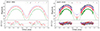 |
Fig. 2. Light curves of J0312 (left) and J1627 (right) folded with the orbital periods and the best-fitting models (solid lines). Two periods are shown for clarity. The orbital phases ϕ = 0.0 correspond to the minima of the models’ brightness. Panels show residuals calculated as the difference between the observed (O) and calculated (C) magnitudes for each data point in terms of the magnitude error, σ. Dashed lines correspond to 3σ levels. |
The fitted parameters are the interstellar reddening (E(B − V)), the distance (D), the pulsar mass (Mp), the component mass ratio (q), the orbit inclination (i), the effective irradiation factor (Kirr), which defines the heating of the companion, the companion Roche lobe filling factor (f), defined as a ratio of distances from the centre of mass of the secondary to the star surface and to the Lagrange point L1, and the companion ‘night-side’ temperature (Tn). We used the mass functions from the radio observations (Table 1) to link the companion mass Mc (or the mass ratio q = Mc/Mp), Mp, and i. The minimum of the χ2 function was determined using the gradient descent method. This approach was preferred as it considerably reduces the computational effort required for the minimisation. The parameter uncertainties were calculated following the method proposed by Lampton et al. (1976). The results are presented in Table 3 and the best-fitting models for both objects are shown by solid lines in Fig. 2.
Light-curve fitting results.
To check whether the model predictions near the J1627 minimum brightness phase are adequate, we combined 20 images at ϕ ≈ 0.00 ± 0.05. Nevertheless, the target was not detected in any band. The corresponding detection limits were gs ≈ 26.9 mag, rs ≈ 26.3 mag, and is ≈ 25.5 mag, which is compatible with the model. For J0312, the number of data points near the minimum brightness phase is not enough to significantly improve the detection limits derived in Sect. 2.1.
4. X-ray data
The J0312 and J1627 fields were observed with Swift/XRT several times between 2010 and 2019 with total exposure times of 5.4 and 8.1 ks, respectively. No statistically significant sources were detected at the pulsars’ positions. Using the Living Swift-XRT Point Source (LSXPS) Upper limit server7 (Evans et al. 2023), we derived the 3σ upper limits on the sources’ count rates of CRJ0312 = 2.2 × 10⁻³ cts s−1 and CRJ1627 = 1.2 × 10⁻³ cts s−1. This corresponds to the unabsorbed fluxes in the 0.5–10 keV range FXJ0312 ≈ 7.9 × 10⁻¹⁴ erg s−1 cm−2 and FXJ1627 ≈ 3 × 10⁻¹⁴ erg s−1 cm−2. Here we assume a power law model with the photon index Γ = 2.5, which is the average value for the BW family (Swihart et al. 2022). The absorbing column densities were  cm−2 and
  cm−2. They were calculated using the reddening values obtained for J0312 and J1627 from the optical fits (Table 3) and the empirical relation from Foight et al. (2016).
The J1627 field was also observed8 with XMM-Newton on 2023 February 10 with duration of 38.5 ks. The European Photon Imaging Camera-Metal Oxide Semiconductor (EPIC-MOS) and EPIC-pn (PN hereafter) detectors were operated in the full frame mode with the thin filter. The XMM-Newton Science Analysis Software (XMM-SAS) v.22.1.0 was utilised for data reduction. The data were reprocessed using the emproc and epproc routines. Unfortunately, the high-energy light curves extracted from the FoVs of detectors showed a significant number of strong background flares. We filtered them out applying the espfilt task. This resulted in effective exposure times of 18.4, 18.8, and 11.2 ks for the MOS1, MOS2, and PN detectors, respectively. Using the edetect_chain tool9 and data from all detectors, we performed source detection. A weak X-ray source, the likely counterpart of J1627, was detected at the pulsar timing position (Fig. 3). Its coordinates are αX = 16h27m53 15 and δX = 32°18′26
 0, and its position uncertainty is 2
 (which combines the statistical uncertainty of 1
 6 and the absolute astrometry accuracy for XMM-Newton/EPIC10 of 1
 2). We also found that the source is not detected in the MOS1 or MOS2 data alone likely due to lower efficiency of the MOS detectors in the soft energy band (≲2 keV) in comparison with the PN camera.
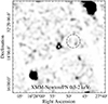 |
Fig. 3. 6′ × 6′XMM-Newton/PN image of the J1627 field in the 0.3–2 keV band. The ‘X’ symbol marks the pulsar timing position from Table 1. The dashed circle shows the region chosen for the background extraction. |
We extracted the source spectrum from the PN data using 10 -radius aperture around its position using the evselect tool. For the background, the 26
 -radius circle was chosen (Fig. 3). The redistribution matrix and ancillary response files were created by the rmfgen and arfgen tasks. We obtained 30.6 net counts in the 0.2–10 keV band and grouped the spectrum to ensure at least 1 count per energy bin. It was fitted in the X-Ray Spectral Fitting Package (XSPEC) v.12.15.0 (Arnaud 1996), applying the W-statistics appropriate for Poisson data with Poisson background11 and the power law model. The tbabs model with the wilm abundances (Wilms et al. 2000) was also included to account for the interstellar absorption. The absorbing column density was fixed at the value mentioned above. As a result, we derived the photon index Γ = 3.3 ± 0.5, the unabsorbed flux in the 0.5–10 keV band and W/d.o.f. = 25/24 (uncertainties are at 1σ confidence). The flux value is in agreement with the upper limit obtained from the Swift data.
5. Discussion and conclusions
We carried out the first multi-band time-series optical photometry of J0312 and J1627. The light curves of both systems are rather symmetric and have one peak per orbital period with a peak-to-peak amplitude of ≳2 mag, which is typical for the BW family (Swihart et al. 2022; Mata Sánchez et al. 2023). The curves can be described by the direct heating model. We note that there is a hint of some deviation from the model seen in the residuals for both objects. This can be caused by different effects, such as cold spots on the donor star surface (Clark et al. 2021), heating by the intra-binary shock (Romani & Sanchez 2016), and heat redistribution over the companion surface via convection and diffusion (Kandel & Romani 2023; Voisin et al. 2020). However, the significance of these possible features is low, and further investigations are necessary to confirm or reject them.
The companions in both systems have very low masses ( M⊙ and
  M⊙), which is typical for the BW population (Swihart et al. 2022). Their temperatures are also compatible with those obtained for BWs (Mata Sánchez et al. 2023); the J0312 companion may have one of the lowest ‘night-side’ temperatures (≈1600 K) of the known BWs.
For a significant number of spider pulsars, dispersion measure (DM) distances are compatible with the parallax distances or are lower than them (see Fig. 5 in Koljonen & Linares 2023). The same situation occurs for our targets: for J1627 the distance provided by the optical fit (4.6 kpc) is close to the DM one (4.5 kpc), while for J0312 it is much greater (2.5 vs 0.8 kpc).
The reddening value for J1627 obtained from the optical fit (Table 3) is in agreement with the maximal E(B − V)≈0.04 mag derived from the 3D dust map of Green et al. (2019). For J0312, the maximal E(B − V) is about 0.1 mag, which is less than the best-fitting value. However, inspection of the map shows that the interstellar medium in the J0312 circumstance is rather non-uniform, providing a E(B − V) of up to ≈0.2 mag. There are no main-sequence stars at distances ≳2.1 kpc, and the star density in the pulsar field is low. Thus, the map results can be dubious. In addition, the uncertainties of the model reddening are quite large.
The J0312 and J1627 proper motions derived from the radio timing are μJ0312 = 33.0 ± 1.4 mas yr−1 and μJ1627 = 3.2 ± 1.4 mas yr−1. The J1627 transverse velocity corresponding to the distance 4.6 kpc from the optical fit is vt ≈ 70 km s−1. This value is compatible with typical binary pulsar velocities, which are mostly lower than 150 km s−1 (Hobbs et al. 2005). In contrast, J0312 has a transverse velocity of ≈400 km s−1 at 2.5 kpc, which is considerably higher than, for example, the vt = 326 km s−1 of the high-velocity MSP PSR B1257+12 (Yan et al. 2013). Moreover, correction for the Shklovskii effect (Shklovskii 1970) and acceleration due to differential Galactic rotation (Nice & Taylor 1995; Lynch et al. 2018) leads to a negative intrinsic Ṗ value. This implies that either the distance or the proper motion is overestimated. Formally, the DM distance of 0.8 kpc provides an acceptable positive Ṗ and vt. However, a smaller distance implies a smaller intrinsic flux of the companion, leading to an unreasonably small companion radius of ∼(25–30) × 103 km. Reliable measurements of the proper motion require a close distance and/or long time base of observations. Dispersion measure variations and timing noise can also lead to inaccurate calculations. For this reason, the J0312 proper motion may be overestimated similar to that of, for example, BW PSR J1641+8049. An updated timing solution for this pulsar yielded a significantly lower proper motion than the previous estimate, allowing us to rule out the spin-up scenario (Kirichenko et al. 2024).
According to the Fermi LAT 14-Year Point Source Catalog DR 4, the J0312 and J1627 fluxes in the 0.1–100 GeV range are  erg s−1 cm−2 and
  erg s−1 cm−2 (Ballet et al. 2023). Using the distances from Table 3, we calculated the corresponding luminosities: LγJ0312 = 4.2 × 1033 erg s−1 and LγJ1627 ≈ 1034 erg s−1. The 3σ upper limit on the J0312 X-ray luminosity is LXJ0312 < 5.9 × 1031 erg s−1. The X-ray luminosity of J1627 is LXJ1627 ≈ 1.1 × 1031 erg s−1. These values are consistent with those of other BWs (Swihart et al. 2022; Koljonen & Linares 2023). The J1627 photon index of ≈3.3 is also typical for a BW. It is high enough to suggest the presence of a thermal component originating from the heated polar caps, although due to the low count statistics we cannot draw any definite conclusions.
The γ-ray and X-ray efficiencies calculated using the observed spin-down luminosities for J0312 are  and
and  and for J1627 – ηγJ1627 = 0.48 and ηXJ1627 = 5 × 10⁻⁴. While the X-ray efficiencies are reasonable for BWs, the γ-ray and irradiation efficiencies are very high. This might be explained by the fact that here we used the observed values of the spin-down luminosity, whereas the intrinsic values can be significantly different. The correction for the acceleration due to differential Galactic rotation is small and does not critically change Ė. The Shklovskii effect for J1627 is also negligible. However, if the pulsars have masses higher than the canonical value of 1.4 M⊙, then their true Ė can essentially be higher. For example, for a pulsar radius of 12–13 km and a mass of 1.7 M⊙, which is a lower bound for both objects (see Table 3), the intrinsic Ė will be ∼2 times higher12.
The next generation of instruments should help us better constrain the parameters of the systems.
Proposal GTC14-23BMEX, PI A. Kirichenko.
Proposal GTC6-24AMEX, PI A. Kirichenko.
αn is the angle between the incoming flux and the normal to the secondary surface, Ω = πRp2/a2 is the solid angle from which the pulsar is visible from the secondary, and a is the orbit separation, Kirr is the effective irradiation factor of the secondary, and σ is the Stefan-Boltzmann constant.
ObsID 0902730101, PI P. Saz Parkinson.
Here we applied the formula from Ravenhall & Pethick (1994).
Acknowledgments
We thank the anonymous referee for useful comments. The work is based on observations made with the Gran Telescopio Canarias (GTC), installed at the Spanish Observatorio del Roque de los Muchachos of the Instituto de Astrofísica de Canarias, on the island of La Palma and on observations obtained with XMM-Newton, a ESA science mission with instruments and contributions directly funded by ESA Member States and NASA. This work made use of data supplied by the UK Swift Science Data Centre at the University of Leicester. This work has made use of data from the European Space Agency (ESA) mission Gaia (https://www.cosmos.esa.int/gaia), processed by the Gaia Data Processing and Analysis Consortium (DPAC, https://www.cosmos.esa.int/web/gaia/dpac/consortium). Funding for the DPAC has been provided by national institutions, in particular the institutions participating in the Gaia Multilateral Agreement. The work of AVB, DAZ and YAS (optical data reduction) was supported by the baseline project FFUG-2024-0002 of the Ioffe Institute. The analysis of the X-ray data by AVK was supported by the Russian Science Foundation project 22-12-00048-P. AK acknowledges the DGAPA-PAPIIT grant IA105024. SVZ acknowledges the DGAPA-PAPIIT grant IN119323. DAZ thanks Pirinem School of Theoretical Physics for hospitality.
References
- Almeida, A., Anderson, S. F., Argudo-Fernández, M., et al. 2023, ApJS, 267, 44 [NASA ADS] [CrossRef] [Google Scholar]
- Alpar, M. A., Cheng, A. F., Ruderman, M. A., & Shaham, J. 1982, Nature, 300, 728 [NASA ADS] [CrossRef] [Google Scholar]
- Arnaud, K. A. 1996, in Astronomical Data Analysis Software and Systems V, eds. G. H. Jacoby, & J. Barnes, Astronomical Society of the Pacific Conference Series, 101, 17 [NASA ADS] [Google Scholar]
- Ballet, J., Bruel, P., Burnett, T. H., & Lott, B., & The Fermi-LAT collaboration 2023, arXiv e-prints [arXiv:2307.12546] [Google Scholar]
- Benvenuto, O. G., De Vito, M. A., & Horvath, J. E. 2014, ApJ, 786, L7 [NASA ADS] [CrossRef] [Google Scholar]
- Bisnovatyi-Kogan, G. S., & Komberg, B. V. 1974, Soviet Astron., 18, 217 [NASA ADS] [Google Scholar]
- Bobakov, A. V., Kirichenko, A. Y., Zharikov, S. V., et al. 2024, A&A, 690, A173 [NASA ADS] [CrossRef] [EDP Sciences] [Google Scholar]
- Cabrera-Lavers, A., Pérez-García, A., Abril Abril, M., Bongiovanni, A., & Cepa, G. 2014, Canarian Observatories Updates CUps, 3, https://www.gtc.iac.es/instruments/osiris/media/CUPS_BBpaper.pdf [Google Scholar]
- Chen, H.-L., Chen, X., Tauris, T. M., & Han, Z. 2013, ApJ, 775, 27 [NASA ADS] [CrossRef] [Google Scholar]
- Claret, A., Hauschildt, P. H., & Witte, S. 2012, A&A, 546, A14 [NASA ADS] [CrossRef] [EDP Sciences] [Google Scholar]
- Claret, A., Hauschildt, P. H., & Witte, S. 2013, A&A, 552, A16 [NASA ADS] [CrossRef] [EDP Sciences] [Google Scholar]
- Clark, C. J., Nieder, L., Voisin, G., et al. 2021, MNRAS, 502, 915 [NASA ADS] [CrossRef] [Google Scholar]
- Dhillon, V. S., Marsh, T. R., Bezawada, N., et al. 2016, in Ground-based and Airborne Instrumentation for Astronomy VI, eds. C. J. Evans, L. Simard, & H. Takami, Society of Photo-Optical Instrumentation Engineers (SPIE) Conference Series, 9908, 99080Y [Google Scholar]
- Dhillon, V., Dixon, S., Gamble, T., et al. 2018, in Ground-based and Airborne Instrumentation for Astronomy VII, eds. C. J. Evans, L. Simard, & H. Takami, Society of Photo-Optical Instrumentation Engineers (SPIE) Conference Series, 10702, 107020L [NASA ADS] [Google Scholar]
- Dhillon, V. S., Bezawada, N., Black, M., et al. 2021, MNRAS, 507, 350 [NASA ADS] [CrossRef] [Google Scholar]
- Draghis, P., Romani, R. W., Filippenko, A. V., et al. 2019, ApJ, 883, 108 [NASA ADS] [CrossRef] [Google Scholar]
- Evans, P. A., Page, K. L., Beardmore, A. P., et al. 2023, MNRAS, 518, 174 [Google Scholar]
- Flewelling, H. A., Magnier, E. A., Chambers, K. C., et al. 2020, ApJS, 251, 7 [NASA ADS] [CrossRef] [Google Scholar]
- Foight, D. R., Güver, T., Özel, F., & Slane, P. O. 2016, ApJ, 826, 66 [Google Scholar]
- Gaia Collaboration (Vallenari, A., et al.) 2023, A&A, 674, A1 [NASA ADS] [CrossRef] [EDP Sciences] [Google Scholar]
- Ginzburg, S., & Quataert, E. 2020, MNRAS, 495, 3656 [Google Scholar]
- Ginzburg, S., & Quataert, E. 2021, MNRAS, 500, 1592 [Google Scholar]
- Green, G. M., Schlafly, E., Zucker, C., Speagle, J. S., & Finkbeiner, D. 2019, ApJ, 887, 93 [NASA ADS] [CrossRef] [Google Scholar]
- Guo, Y., Wang, B., & Han, Z. 2022, MNRAS, 515, 2725 [NASA ADS] [CrossRef] [Google Scholar]
- Guo, Y., Wang, B., & Li, X. 2024, MNRAS, 527, 7394 [Google Scholar]
- Hobbs, G., Lorimer, D. R., Lyne, A. G., & Kramer, M. 2005, MNRAS, 360, 974 [Google Scholar]
- Honeycutt, R. K. 1992, PASP, 104, 435 [NASA ADS] [CrossRef] [Google Scholar]
- Kandel, D., & Romani, R. W. 2023, ApJ, 942, 6 [Google Scholar]
- Kilic, M., Bédard, A., Bergeron, P., & Kosakowski, A. 2020, MNRAS, 493, 2805 [NASA ADS] [CrossRef] [Google Scholar]
- Kirichenko, A. Y., Zharikov, S. V., Karpova, A. V., et al. 2024, MNRAS, 527, 4563 [Google Scholar]
- Koljonen, K. I. I., & Linares, M. 2023, MNRAS, 525, 3963 [NASA ADS] [CrossRef] [Google Scholar]
- Koljonen, K. I. I., & Linares, M. 2025, ApJ, accepted [arXiv:2505.11691] [Google Scholar]
- Lampton, M., Margon, B., & Bowyer, S. 1976, ApJ, 208, 177 [Google Scholar]
- Li, D., Wang, P., Hou, X., et al. 2022, Joint Pulsar Studies with the FAST radio telescope and the Fermi LAT, https://indico.cern.ch/event/1091305/contributions/5007590/attachments/2530789/4354373/221010_Saz_Parkinson_10thFSymp_opt.pdf [Google Scholar]
- Lynch, R. S., Swiggum, J. K., Kondratiev, V. I., et al. 2018, ApJ, 859, 93 [NASA ADS] [CrossRef] [Google Scholar]
- Manchester, R. N., Hobbs, G. B., Teoh, A., & Hobbs, M. 2005, AJ, 129, 1993 [Google Scholar]
- Mata Sánchez, D., Kennedy, M. R., Clark, C. J., et al. 2023, MNRAS, 520, 2217 [CrossRef] [Google Scholar]
- Naylor, T. 1998, MNRAS, 296, 339 [NASA ADS] [CrossRef] [Google Scholar]
- Nice, D. J., & Taylor, J. H. 1995, ApJ, 441, 429 [NASA ADS] [CrossRef] [Google Scholar]
- Oke, J. B. 1990, AJ, 99, 1621 [Google Scholar]
- Prša, A. 2018, Modeling and Analysis of Eclipsing Binary Stars; The theory and design principles of PHOEBE (Bristol, UK: IOP Publishing) [Google Scholar]
- Ravenhall, D. G., & Pethick, C. J. 1994, ApJ, 424, 846 [NASA ADS] [CrossRef] [Google Scholar]
- Roberts, M. S. E. 2013, in Neutron Stars and Pulsars: Challenges and Opportunities after 80 years, ed. J. van Leeuwen, IAU Symposium, 291, 127 [Google Scholar]
- Romani, R. W., & Sanchez, N. 2016, ApJ, 828, 7 [Google Scholar]
- Saz Parkinson, P. 2021, The X-ray counterpart of PSR J1627+3219, a new MSP discovered by FAST, XMM-Newton Proposal ID #90273 [Google Scholar]
- Shklovskii, I. S. 1970, Soviet Ast., 13, 562 [NASA ADS] [Google Scholar]
- Smith, J. A., Tucker, D. L., Kent, S., et al. 2002, AJ, 123, 2121 [NASA ADS] [CrossRef] [Google Scholar]
- Smith, D. A., Abdollahi, S., Ajello, M., et al. 2023, ApJ, 958, 191 [NASA ADS] [CrossRef] [Google Scholar]
- Swihart, S. J., Strader, J., Chomiuk, L., et al. 2022, ApJ, 941, 199 [NASA ADS] [CrossRef] [Google Scholar]
- Tabassum, S., Ransom, S., Ray, P., et al. 2021, in 43rd COSPAR Scientific Assembly. Held 28 January– 4 February, 43, 1208 [Google Scholar]
- van Dokkum, P. G. 2001, PASP, 113, 1420 [Google Scholar]
- Voisin, G., Kennedy, M. R., Breton, R. P., Clark, C. J., & Mata-Sánchez, D. 2020, MNRAS, 499, 1758 [NASA ADS] [CrossRef] [Google Scholar]
- Wilms, J., Allen, A., & McCray, R. 2000, ApJ, 542, 914 [Google Scholar]
- Yan, Z., Shen, Z.-Q., Yuan, J.-P., et al. 2013, MNRAS, 433, 162 [CrossRef] [Google Scholar]
- Yao, J. M., Manchester, R. N., & Wang, N. 2017, ApJ, 835, 29 [NASA ADS] [CrossRef] [Google Scholar]
- Zharikov, S., Tovmassian, G., Aviles, A., et al. 2013, A&A, 549, A77 [NASA ADS] [CrossRef] [EDP Sciences] [Google Scholar]
- Zharikov, S., Kirichenko, A., Zyuzin, D., Shibanov, Y., & Deneva, J. S. 2019, MNRAS, 489, 5547 [CrossRef] [Google Scholar]
All Tables
All Figures
|
Fig. 1. Optical images of the fields of the two pulsars. Top panel: 3 |
| In the text | |
|
Fig. 2. Light curves of J0312 (left) and J1627 (right) folded with the orbital periods and the best-fitting models (solid lines). Two periods are shown for clarity. The orbital phases ϕ = 0.0 correspond to the minima of the models’ brightness. Panels show residuals calculated as the difference between the observed (O) and calculated (C) magnitudes for each data point in terms of the magnitude error, σ. Dashed lines correspond to 3σ levels. |
| In the text | |
|
Fig. 3. 6′ × 6′XMM-Newton/PN image of the J1627 field in the 0.3–2 keV band. The ‘X’ symbol marks the pulsar timing position from Table 1. The dashed circle shows the region chosen for the background extraction. |
| In the text | |
Current usage metrics show cumulative count of Article Views (full-text article views including HTML views, PDF and ePub downloads, according to the available data) and Abstracts Views on Vision4Press platform.
Data correspond to usage on the plateform after 2015. The current usage metrics is available 48-96 hours after online publication and is updated daily on week days.
Initial download of the metrics may take a while.