| Issue |
A&A
Volume 703, November 2025
|
|
|---|---|---|
| Article Number | A8 | |
| Number of page(s) | 9 | |
| Section | Planets, planetary systems, and small bodies | |
| DOI | https://doi.org/10.1051/0004-6361/202554006 | |
| Published online | 30 October 2025 | |
Radius valley scaling among low-mass stars with TESS
1
Departamento de Astronomía, Universidad de Chile,
Camino El Observatorio 1515, Las Condes,
Santiago,
Chile
2
Instituto de Astrofisica, Pontificia Universidad Católica de Chile,
Av. Vicuña Mackenna 4860,
7820436
Macul, Santiago,
Chile
★ Corresponding author: This email address is being protected from spambots. You need JavaScript enabled to view it.
Received:
3
February
2025
Accepted:
27
August
2025
Abstract
The Transiting Exoplanet Survey Satellite (TESS) has been highly successful in detecting planets in close orbits around low-mass stars, particularly M dwarfs. This presents a valuable opportunity to conduct detailed population studies to understand how these planets depend on the properties of their host stars. The previously observed radius valley in Sun-like stars has also been observed among M dwarfs; however, how its properties vary when compared with more massive stars remains uncertain. We select the volume limited Bioverse stellar catalog, with precise photometric stellar parameters, which was cross-matched with the planet catalog consisting of TESS objects of interests (TOI) candidates and confirmed planets. We detect the radius valley around M dwarfs at a location of 1.64 ± 0.03 R⊕ and with a depth of approximately 45%. The radius valley among GKM stars scales with stellar mass as Rp ∝ M∗0.15±0.04. The slope is consistent, within 0.3σ, with those around Sun-like stars. For M dwarfs, the discrepancy is 3.6σ with the extrapolated slope from the Kepler FGK sample, marking the point where the deviation from previous results begins. Moreover, we do not see a clear shift in the radius valley between early and mid M dwarfs. The flatter scaling of the radius valley for lower-mass stars suggests that mechanisms other than atmospheric mass loss through photoevaporation may shape the radius distribution of planets around M dwarfs. A comparison of the slope with various planet formation and evolution models leads to a good match with pebble accretion models including water worlds, indicating a potentially different regime of planet formation that can be probed with exoplanets around the lowest-mass stars.
Key words: catalogs / planets and satellites: composition / planets and satellites: dynamical evolution and stability / planets and satellites: formation / planets and satellites: physical evolution / planets and satellites: terrestrial planets
© The Authors 2025
 Open Access article, published by EDP Sciences, under the terms of the Creative Commons Attribution License (https://creativecommons.org/licenses/by/4.0), which permits unrestricted use, distribution, and reproduction in any medium, provided the original work is properly cited.
This article is published in open access under the Subscribe to Open model. This email address is being protected from spambots. You need JavaScript enabled to view it. to support open access publication.
1 Introduction
Over the past decade, planet detections through the transit method have significantly increased, facilitated by missions such as the Kepler spacecraft and the Transiting Exoplanet Survey Satellite (TESS) (Ricker et al. 2015). Kepler and its extended mission, K2 (Borucki et al. 2010; Batalha et al. 2013; Howell et al. 2014; Thompson et al. 2018), have discovered more than 2800 confirmed planets, with an additional 3000 candidates yet to be confirmed. This large dataset enables comprehensive population studies of planetary architectures (e.g. Mulders et al. 2018; Dattilo et al. 2023). Demographic studies indicate that more than half of Sun-like star hosts at least one low-mass, short-period planet (Borucki et al. 2010; Batalha et al. 2011; He et al. 2019). The occurrence rates of planets smaller than Neptune are particularly high around low-mass stars (Dressing & Charbonneau 2013, 2015; Mulders et al. 2015; Hsu et al. 2020).
By accurately measuring the stellar parameters, the properties of planets can be measured more precisely, allowing for additional features to be detected. With precise radius measurements from the California-Kepler Survey (Petigura et al. 2017), a deficit of planets at approximately 1.7 R⊕ around Sun-like stars was observed (Fulton et al. 2017). This radius valley divides the planets into two groups: super-Earths and mini-Neptunes. This corresponds with an earlier discovery that the densities of small planets are divided into similar categories, with the smaller super-Earths with a rocky core with a thin or no atmospheres and the mini-Neptunes with rocky cores and thick atmospheres (Rogers 2015; Wolfgang et al. 2016).
The radius valley provides insights into planet formation and evolution around various types of stars, with several mechanisms proposed to explain its origin. Photoevaporation, the most accepted process, involves extreme ultraviolet radiation stripping away hydrogen-helium envelopes over time, leading to smaller planetary radii (Owen & Wu 2017; Owen & Murray-Clay 2018; Wu 2019; Rogers et al. 2021). Core-powered mass loss, described by Ginzburg et al. (2018), Gupta & Schlichting (2019), and Gupta & Schlichting (2020), relies on the planet’s residual core luminosity and incident bolometric flux eroding its atmosphere over time, resulting in bare rocky core planets. However, Tang et al. (2024) found that outside the boil-off phase, the core-powered escape is not able to drive significant mass loss.
Alternatively, a dichotomy in planet core composition between rocky and water worlds (e.g. Izidoro et al. 2022) could also create a radius valley. Planet formation models integrate pebble accretion with photoevaporation following disk dispersal, accounting for the presence of water worlds to explain the presence of a radius valley among low-mass stars (Venturini et al. 2024; Nielsen et al. 2025). Other planet formation-evolution models have also been put forth to explain the cause of the radius valley, such as impact erosion (Wyatt et al. 2019) and late planet formation in either gas-poor or even gas-empty disks (Lopez & Rice 2018; Lee & Connors 2021; Lee et al. 2022). Among these, photoevaporation and water worlds have emerged as the dominant explanations for planets around solar-mass stars.
Wu (2019) observed that the radius valley among Kepler’s FGK stars shifts to smaller radii as the stellar mass decreases, and found a power law dependence between the two, ![Mathematical equation: $\[R_{p} ~\alpha~ M_{*}^{\beta}\]$](/articles/aa/full_html/2025/11/aa54006-25/aa54006-25-eq2.png) , with β ∈ [0.95, 1.40] due to photoevaporation among Kepler planets. This linear dependence for FGKM stars has also been explained by core-powered mass loss as observed by Berger et al. (2020) through a slope of β =
, with β ∈ [0.95, 1.40] due to photoevaporation among Kepler planets. This linear dependence for FGKM stars has also been explained by core-powered mass loss as observed by Berger et al. (2020) through a slope of β = ![Mathematical equation: $\[0.26_{-0.16}^{+0.21}\]$](/articles/aa/full_html/2025/11/aa54006-25/aa54006-25-eq3.png) . Bonfanti et al. (2023) observe ∂ log Rp-valley/∂ log M⋆ ≈ 0.23 and 0.27 for the photo-evaporation and core-powered mass-loss models, respectively. The difference between the two inferences from the observations suggests other possible mechanisms that shape the radius valley. Ho & Van Eylen (2023) also notes that thermally driven mass-loss models predict a similar dependence of the valley on stellar mass, based on observations of FGK stars from Kepler. When we extend the sample from FGK to M dwarfs, the planet formation model proposed by Venturini et al. (2024) integrating pebble accretion with photoevaporation following disk dispersal results in a scaling of
. Bonfanti et al. (2023) observe ∂ log Rp-valley/∂ log M⋆ ≈ 0.23 and 0.27 for the photo-evaporation and core-powered mass-loss models, respectively. The difference between the two inferences from the observations suggests other possible mechanisms that shape the radius valley. Ho & Van Eylen (2023) also notes that thermally driven mass-loss models predict a similar dependence of the valley on stellar mass, based on observations of FGK stars from Kepler. When we extend the sample from FGK to M dwarfs, the planet formation model proposed by Venturini et al. (2024) integrating pebble accretion with photoevaporation following disk dispersal results in a scaling of ![Mathematical equation: $\[R_{p} \propto M_{\star}^{0.14}\]$](/articles/aa/full_html/2025/11/aa54006-25/aa54006-25-eq4.png) . In this paper, we revisit the radius valley among the TESS planet candidates around GKM stars, to extend the scaling relation of the radius valley to lower-mass stars to put tighter constraints on the different proposed hypotheses among the planet size and stellar mass within low-mass stars.
. In this paper, we revisit the radius valley among the TESS planet candidates around GKM stars, to extend the scaling relation of the radius valley to lower-mass stars to put tighter constraints on the different proposed hypotheses among the planet size and stellar mass within low-mass stars.
Despite being optimized for detecting planets around Sunlike stars, the Kepler mission also observed a small number of M dwarfs (Dressing & Charbonneau 2013). This limited sample yielded intriguing results, revealing that M dwarfs host more small transiting planets than Sun-like stars (Mulders et al. 2015; Dressing & Charbonneau 2015). However, due to the small sample size (approximately 85 confirmed Kepler planets around M dwarfs), a larger dataset, such as that provided by TESS, is crucial for better studies. The launch of TESS, with its extensive sky coverage and wide, red optical bandpass filter, is particularly suited to observing M dwarfs (Ballard 2019; Barclay et al. 2018), which are cool and red. Most nearby stars are M dwarfs, presenting a significant opportunity to detect and study planets around the lowest-mass stars (Figure 1).
With 7341 planet candidates from TESS1, we now have a large dataset for demographic studies. Precise stellar parameters are needed to calculate accurate planet radii and pinpoint the radius valley across different stellar types (e.g. Berger et al. 2020). M dwarfs, specifically, are known to have a fading radius valley (Cloutier & Menou 2020; Ho et al. 2024; Gaidos et al. 2024; Parc et al. 2024), attributing to planet migration. Therefore, we wanted to revisit the radius valley for the M dwarfs, to better constrain planet formation-evolution models.
In this work, we focus on a volume-limited sample of TESS planet candidate hosts with photometric stellar parameters from the Bioverse catalog (Hardegree-Ullman et al. 2023) (Section 2.1) to calculate their planet radii within 3% of precision. We employ a Gaussian mixture model, GMM (Section 2.2), to measure the locations of super-Earth and mini-Neptune peaks and the radius valley among GKM type stars. Subsequently, we further analyze the shift in the location of the radius valley with stellar mass (Section 3) and discuss the final results and conclusions (Section 4).
2 Methods
2.1 Low-mass star sample
For exoplanet demographics, homogeneous stellar samples are needed. The Bioverse, a volume-limited sample (up to 120 pc), based on Gaia DR3 (Gaia Collaboration 2023) parallaxes and photometry, has updated stellar parameters, which we utilized to refine the properties of TESS input catalog (TIC) planet hosts (Stassun et al. 2018; Stassun et al. 2019). The use of the Bioverse catalog helped bring down the uncertainties to 1% in effective stellar temperature, 3% in stellar radius, and 5.5% in stellar mass.
We cross-matched the coordinates (right ascension and declination) and the GAIA IDs of the stars within 120 pc and with effective temperatures up to 7000 K between the Bioverse and TESS TOI catalogs, resulting in 457 planet candidates and 257 confirmed planets associated with GKM stellar types (properties of our sample in Table 1). No specific cuts were applied to the sample, other than stellar temperature and distance. We then used these stellar parameters to recalculate the planet radius ![Mathematical equation: $\[\left(R_{p}^{\prime}=R_{p} *\left(R_{\star}^{\prime} / R_{\star}\right)\right)\]$](/articles/aa/full_html/2025/11/aa54006-25/aa54006-25-eq5.png) . By recalculating the radius of the planet, we reduced the uncertainty of the planet radius from 7.29% to 3.98%, which accounts for the transit depth and the stellar radius uncertainty of 2.6% and 3%, respectively.
. By recalculating the radius of the planet, we reduced the uncertainty of the planet radius from 7.29% to 3.98%, which accounts for the transit depth and the stellar radius uncertainty of 2.6% and 3%, respectively.
To ensure that there were enough planets to characterize the radius valley, we included all of the confirmed and candidate planets from the TOI list. We excluded the false positives and false alarms from our sample, using the disposition column from the TESS Follow-up Observing Program Working Group (TFOPWG) in the TOI catalog, as most of these were in the 0.5–6 R⊕ range. We also conducted a Triceratops run (Giacalone et al. 2021) to assess the likelihood of false positives. The results (Appendix B) showed no significant differences between the likely planets and the set of planet candidates identified by Triceratops. Therefore, we chose to proceed with the larger sample that includes planet candidates. While some false positives may still be present in our sample, we prefer the trade-off of having a larger sample size, at the potential cost of lower reliability, to perform our analysis over a reliable and small sample. This results in a larger sample size when compared with previous studies of planet radii distributions (Parc et al. 2024; Gaidos et al. 2024). In Appendix B, we show that when only known and confirmed planets are used for the analysis, the results are consistent within errors; however, by including the candidate planets into our sample, we increase the planet sample for a more robust statistical analysis and reduce errors from the statistics of the small sample.
We also ensured that our analysis is not contaminated by binaries. To check for binary stars in our star sample, we looked into the renormalized unit weight error (RUWE) parameter from the GAIA mission (Lindegren 2018), which is typically used as an indicator of multiplicity. Looking at the distribution of RUWE, stars with values >1.4 are considered to be possible unresolved binaries. In the Bioverse catalog we used, there are a total of 286 391 stars among which only 54 267 stars have a RUWE value greater than 1.4. So, 19% of the stars in the Bioverse catalog could be unresolved binaries. In the Bioverse-TOI sample we identify 64 possible binaries, with a 9% probability. This lower fraction likely means binaries have partly been eliminated during the vetting process. We have kept possible binaries in our sample but verified throughout the paper that omitting them does not significantly impact the analysis of the planet radius distribution.
Table 2 shows our sample, from this dataset, we divided the 843 planet candidates into three temperature bins corresponding to stellar types: M dwarfs (Teff < 3880 K), K dwarfs (Teff < 5340 K), and G dwarfs (Teff < 6040 K). This categorization resulted in 327 M dwarfs, 304 K dwarfs, and 165 G dwarfs. The relatively low number of G dwarfs is a result of the volume limit of the Bioverse catalog.
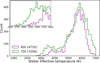 |
Fig. 1 Histogram comparing TESS objects of interest (TOIs) and Kepler objects of interest (KOIs) from the NASA Exoplanet Archive, with star counts indicated in parentheses. The inset plot (top left) highlights the significant increase in low-mass stars identified by TESS, which enhances our ability to study these stars in greater detail. |
Summary of the stellar properties (median values) included in this study.
Stellar and planet properties of all the targets in our sample.
2.2 Planet radii distribution
Figure 2 shows the planet radii distribution of the 667 GKM dwarfs hosting planets between 1 and 3 R⊕ (after excluding the false alarms and false positives from the TESS Follow-up Observing Program Working Group (TFOPWG) disposition column). Radius valleys around M dwarfs and G dwarfs are clearly observed at 1.63 R⊕ and 1.86 R⊕. Around K dwarfs, the radius valley at 1.76 R⊕ is less prominent, possibly due to the relatively low number of super-Earths compared to the number of mini-Neptunes. Because the prominence of the radius valley in the histograms can depend on the choice of bins, we use a KDE and GMM approach and recover the radius valley.
We note that our sample has not been corrected for completeness. Completeness correction can change the relative height of the super-Earth and mini-Neptune peaks, thereby shifting the inferred value of the radius gap to lower or upper values. So, we used the Fulton et al. (2017) dataset to assess the impact of completeness correction on the radius gap and found that the effect was within uncertainties. Therefore, we proceeded with the raw sample, which includes both confirmed and candidate planets.
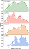 |
Fig. 2 Kernel density estimates along with the histograms of olanet radii distribution of the entire sample and M, K, G stellar types. |
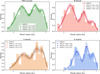 |
Fig. 3 GMM fits to the unbinned radius data, along with corresponding histograms, are presented for the entire low-mass star sample and for M, K, and G stellar types. The super-Earth and mini-Neptune peaks, as well as the radius valley, are indicated in each plot. |
2.2.1 Kernel density estimates (KDEs)
Figure 2 shows the KDEs of the planet radii distribution along with their histograms revealing the radius valley. Due to the 3.98% uncertainty in the radius measurements, the histogram binning had to be carefully adjusted to accurately capture the radius gap. By adjusting the bandwidth from 0.2 to 0.3, we selected the KDEs that best represent the data. The KDEs helped in representing the bimodality in the planet radii distribution of the small sample space of M, K, G stellar types.
We observe a subtle valley in both the histogram and KDE around 1.7 R⊕ for the entire sample, consistent with the known bimodal planet radius distribution (Fulton et al. 2017). The radius valley is not deep, with a minimum of 45%, consistent with shape of the valley in a more heterogeneous sample of host stars. The absence of a well-defined deep radius gap among the planets can be attributed to low number statistics and possible contamination of the sample with false positives. Similarly, radius valleys are clearly observed for the individual G, K, and M stellar spectral types. M dwarfs exhibit a distinct valley, with a small sub-Neptune peak, consistent with previous studies. For K dwarfs, despite the sample containing around 300 planets, the radius valley is not as clearly seen in the histogram compared to M dwarfs, mostly due to a relatively low number of detected super-Earths compared to mini-Neptunes. G dwarfs, however, present a clearer distinction between mini-Neptunes and super-Earths, with evident support for the radius valley.
2.2.2 Gaussian mixture models (GMMs)
To accurately estimate the location of the radius valley, we used the GMM from the sklearn.mixture package. A GMM is a probabilistic model that assumes that data points are generated from a mixture of a finite number of Gaussian distributions with unknown parameters. We implemented the GMM fit to the planet radii values in the range, 0.8–3.2 R⊙ and evaluated the fit of the GMM, using the Bayesian information criterion (BIC), to help determine the goodness of fit. The bootstrapping resampling method was used to account for uncertainties in the data by generating multiple versions of the radius distribution and seeing how sensitive the GMM’s features are to the omission of specific data points.
The radius valleys for the stellar types are presented in Figure 3. We explored a different number of components (two, three, and more), and found that a three-component model provides a better fit to the region around the radius valley (refer Appendix A). In all cases, the location of the first minimum aligns well with the radius valley seen in the histograms and KDEs. The derived locations and their confidence intervals are listed in Table 3. The valley shifts to smaller radii for later spectral types, a trend we explore further in the next section.
Super-Earth peaks, mini-Neptune peaks, and radius valley values from two- and three-component GMM fits for the entire sample and M, K, and G dwarfs.
 |
Fig. 4 Slope values, |
![Mathematical equation: $\[\beta=\left(\frac{\partial ~\log~ R_{\mathrm{gap}}}{\partial ~\log~ M_*}\right)\]$](/articles/aa/full_html/2025/11/aa54006-25/aa54006-25-eq6.png)
3 Planet size scaling with stellar mass
We performed a nonlinear least squares fit to quantify the relationship between planet size and stellar mass, observed through the GMM analysis of the G, K, and M stars. The shift of the radius valley to smaller radius values along decreasing stellar masses gave us a power-law scaling of ![Mathematical equation: $\[R_{\text {valley }}=1.87 * M_{\star}^{\beta}\]$](/articles/aa/full_html/2025/11/aa54006-25/aa54006-25-eq7.png) , β = 0.15 ± 0.04.
, β = 0.15 ± 0.04.
The observed shift of the radius valley with stellar mass aligns with prior observational studies of Kepler and TESS planets (Figure 4). Studies, such as the one of Wu (2019), who found ![Mathematical equation: $\[R_{p} \propto M_{\star}^{0.25}\]$](/articles/aa/full_html/2025/11/aa54006-25/aa54006-25-eq8.png) , and Ho & Van Eylen (2023), who reported β =
, and Ho & Van Eylen (2023), who reported β = ![Mathematical equation: $\[0.23_{-0.064}^{+0.053}\]$](/articles/aa/full_html/2025/11/aa54006-25/aa54006-25-eq9.png) for FGK stars and similarly, Berger et al. (2020) obtained β =
for FGK stars and similarly, Berger et al. (2020) obtained β = ![Mathematical equation: $\[0.26_{-0.16}^{+0.21}\]$](/articles/aa/full_html/2025/11/aa54006-25/aa54006-25-eq10.png) and Petigura et al. (2022) identified a slope of β =
and Petigura et al. (2022) identified a slope of β = ![Mathematical equation: $\[0.18_{-0.07}^{+0.08}\]$](/articles/aa/full_html/2025/11/aa54006-25/aa54006-25-eq11.png) for FGKM stars. A more recent study by Berger et al. (2023) determined a slope of
for FGKM stars. A more recent study by Berger et al. (2023) determined a slope of ![Mathematical equation: $\[\left(\frac{\partial ~\log~ R_{\text{gap}}}{\partial ~\log~ M_{*}}\right)_{S}= -0.046_{-0.117}^{+0.125}\]$](/articles/aa/full_html/2025/11/aa54006-25/aa54006-25-eq12.png) under a constant incident flux (S) for Kepler planets. However, for low-mass stars, Luque & Pallé (2022) observed a slope of β = 0.08 ± 0.12 and Bonfanti et al. (2023) β =
under a constant incident flux (S) for Kepler planets. However, for low-mass stars, Luque & Pallé (2022) observed a slope of β = 0.08 ± 0.12 and Bonfanti et al. (2023) β = ![Mathematical equation: $\[0.054_{-0.034}^{+0.049}\]$](/articles/aa/full_html/2025/11/aa54006-25/aa54006-25-eq13.png) for M dwarfs, within TESS planets.
for M dwarfs, within TESS planets.
While the inferred slope among GKM stars agrees well with that initially inferred from Kepler by Wu (2019), the results for M dwarfs are different. A discrepancy of approximately 3.6σ is observed for the M dwarf data point, pointing to a distinct planet formation and evolution mechanism for these stars (Figure 6). We characterize the radius valley scaling among M dwarfs in more detail in the next paragraph.
In our dataset, we identified approximately 320 M dwarfs with effective temperatures ranging from 2637 to 3870 K, which we here divide into two groups to create early and late M dwarf samples. The early M dwarf group (M0-M3, 3440–3880 K) contains 163 stars, with a median 0.502 M⋆. Similarly, the late M dwarf group (M4–M8, 2630–3440 K) also includes 164 stars, with a median mass of 0.299M⋆. Following the same procedure outlined in Section 2.1, we plotted a histogram along with the GMM fit. We observe a clear radius valley at 1.63 ± 0.08 R⊕ and 1.69 ± 0.12 R⊕ for the early and late M dwarf samples, respectively (Figure 5). The scaling is, within the uncertainties, consistent with β = 0, indicating no evidence of a scaling relationship. However, the uncertainties are sufficiently large that the existence of a scaling cannot be ruled out. Additionally, no evidence of a slope is observed among the M dwarfs.
With the new radius valley values for the early and late M dwarfs, we updated our power-law scaling with these additional points and found a shallower slope of β = 0.12 ± 0.06. Here, we can observe that the new data points are consistent with our previous fit, whereby the slope gets less steep when compared with FGK stars (Figure 6). The comparison with Wu (2019) shows that the slope matches for the Sun-like stars but when M dwarfs are included a diversion is observed. This deviation in the slope of the radius valley may suggest a break in the trend predicted by photoevaporation models for FGK stars. For M dwarfs, this deviation may point to the need for additional mechanisms, such as the inclusion of water worlds or pebble accretion models. The implications of this deviation will be discussed further in Section 4.
 |
Fig. 5 GMM fits along with their histograms for early and late M dwarfs. |
 |
Fig. 6 Comparison of our data with that of Wu (2019). The scaling from Wu is plotted with an offset for better alignment and easier comparison. |
4 Conclusions and discussions
We created a volume-limited sample by cross-matching 7341 TESS project candidates from the TESS exoplanet archive2 with the Bioverse catalog for better precision of stellar effective temperatures and a 3% accurate planet radius measurements of all the TESS TOIs. With this refined sample of 843 planets, we examined the radius valley among the GKM stellar types with histograms, KDEs, and GMMs. We used GMM to measure the location of the radius valley and its associated uncertainty for spectral types M, K, and G. Our main conclusions are:
A clear radius valley is observed among the 327 M dwarfs at a radius of 1.64 ± 0.03 R⊕ and a depth of 45%. Splitting the M dwarf sample into mid and late M dwarfs, with median masses of 0.30 and 0.502 M⊙, respectively, we find the radius valleys at 1.63 ± 0.08 R⊕ and 1.69 ± 0.12 R⊕, respectively.
We find that the location of the radius valley increases with spectral type, ranging from 1.63 ± 0.03 R⊕ for M dwarfs to 1.86 ± 0.06 R⊕ for G dwarfs. By fitting a scaling relation with stellar mass for GKM stars, we derive
![Mathematical equation: $\[R_{p}=M_{\star}^{0.15 \pm 0.04}\]$](/articles/aa/full_html/2025/11/aa54006-25/aa54006-25-eq14.png) . This scaling is shallower than that observed for Kepler FGK stars.
. This scaling is shallower than that observed for Kepler FGK stars.We detect no radius valley scaling with stellar mass among M dwarfs, possibly due to a small sample size (Figure 6). In addition, the location of the valley in M dwarfs is significantly higher than expected based on extrapolating the slope around Kepler FGK stars at 3.6σ.
The steep slope around FGK stars matches well with atmospheric mass loss through photoevaporation. However, the flattening of the slope around M dwarfs may indicate a different mechanism may play a role for lower-mass stars. Our observations match particularly well with the pebble accretion models including water worlds from Venturini et al. (2024).
The larger homogeneous dataset with updated stellar parameters allowed us to clearly identify the radius valley among M dwarfs – a feature that many prior studies missed. Previous studies with datasets containing fewer than 200 planets with mass measurements did not observe this feature clearly or rather observed a fading radius valley among the low-mass stars (e.g. Luque & Pallé 2022; Parc et al. 2024).
The observed power-law scaling from this study, ![Mathematical equation: $\[R_{p} ~\alpha~ M_{*}^{0.15}\]$](/articles/aa/full_html/2025/11/aa54006-25/aa54006-25-eq15.png) , aligns well with previous models and observation studies conducted for Kepler and TESS planets. The slopes obtained for FGK stars by Wu (2019) seem consistent with photoevaporation. Berger et al. (2023) find that core-powered mass-loss dominates over photoevaporation in shaping the radius valley among Kepler planets. Petigura et al. (2022) also found a power-law scaling for FGKM stellar types in support of mass-loss mechanisms. Interestingly, Rogers et al. (2021) found either photoevaporation and core-powered mass-loss models consistent with their two datasets from the California-Kepler Survey and the Gaia-Kepler Survey. However, when M dwarfs are included, the slope seems to get shallower, as is seen in this study and others (Figure 4) (Luque & Pallé 2022; Bonfanti et al. 2023).
, aligns well with previous models and observation studies conducted for Kepler and TESS planets. The slopes obtained for FGK stars by Wu (2019) seem consistent with photoevaporation. Berger et al. (2023) find that core-powered mass-loss dominates over photoevaporation in shaping the radius valley among Kepler planets. Petigura et al. (2022) also found a power-law scaling for FGKM stellar types in support of mass-loss mechanisms. Interestingly, Rogers et al. (2021) found either photoevaporation and core-powered mass-loss models consistent with their two datasets from the California-Kepler Survey and the Gaia-Kepler Survey. However, when M dwarfs are included, the slope seems to get shallower, as is seen in this study and others (Figure 4) (Luque & Pallé 2022; Bonfanti et al. 2023).
The flatter slopes around M dwarfs are predicted by certain planet formation and evolution models. For example, Venturini et al. (2024), who use pebble accretion models to create a population of rocky planets and water worlds, predict a slope of ![Mathematical equation: $\[R_{p} ~\alpha~ M_{*}^{0.14}\]$](/articles/aa/full_html/2025/11/aa54006-25/aa54006-25-eq16.png) . Therefore, it is evident that as we shift toward the lowest-mass stars additional mechanisms such as pebble accretion or the inclusion of water worlds may be necessary to account for the relatively flat slopes, while photoevaporation alone may be insufficient.
. Therefore, it is evident that as we shift toward the lowest-mass stars additional mechanisms such as pebble accretion or the inclusion of water worlds may be necessary to account for the relatively flat slopes, while photoevaporation alone may be insufficient.
A limitation of this analysis is that it is based on a sample of planet candidates that may include an unknown number of false positives. While a large sample size is essential to robustly detect the radius valley across different spectral types, ongoing efforts to validate candidates and remove false positives may influence the results. However, a comparison between confirmed planets and candidates showed no significant differences, so we proceeded with the full sample including candidates.
To evaluate the impact of completeness corrections, we performed a comparison using the Fulton et al. (2017) dataset. We examined the radius valley before and after applying a completeness correction; although the valley remains visually consistent in the histogram, the GMM analysis reveals a slight shift across all stellar types. This shift likely arises from differing completeness corrections between super-Earths and mini-Neptunes, but the planet radius–stellar mass slope remains unaffected. While our volume-limited sample improves homogeneity, we did not apply a completeness correction near the detection threshold. This omission may particularly affect the radius valley detection for K dwarfs, where super-Earths appear underrepresented relative to mini-Neptunes. A more rigorous completeness treatment is needed to refine these results and will be pursued in future work.
Data availability
The full Table 2 is available at the CDS via https://cdsarc.cds.unistra.fr/viz-bin/cat/J/A+A/703/A8.
Acknowledgements
The authors thank the referee for providing insightful comments, that improved this work and made the results clearer. H.M.P acknowledges support from ANID (Beca de doctorado nacional) folio de postulacion 21241689, FONDECYT project 11221206, FONDECYT project 1252141, and from ANID – Millennium Science Initiative – ICN12_009; and would like to thank the thesis committee members for their valuable advice over time. G.D.M. acknowledges support from FONDECYT project 1252141 and the ANID BASAL project FB210003. This research has made use of the NASA Exoplanet Archive, which is operated by the California Institute of Technology, under contract with the National Aeronautics and Space Administration under the Exoplanet Exploration Program. This paper includes data collected by the TESS mission. Funding for the TESS mission is from the NASA Science Mission directorate. The results reported herein benefited from collaborations and/or information exchange within NASA’s Nexus for Exoplanet System Science (NExSS) research coordination network sponsored by NASA’s Science Mission Directorate and project “Alien Earths” funded under Agreement No. 80NSSC21K0593. We also want to thank the TESS team at MIT for all the work done in making the mission happen and the CALTECH team for maintaining the NASA Exoplanet Archive.
Appendix A Gaussian mixture model (GMM)
To obtain the accurate values of the radius valley that we observed in the histograms and KDE, we utilized Gaussian mixture modeling, a package from sklearn.mixture. GMM is a probabilistic model that assumes that all the data points are generated from a mixture of a finite number of Gaussian distributions with unknown parameters. Therefore, we obtain the precise values of the bimodality, such as the Peaks and minima of the fit. The bootstrapping resampling method was used to account for uncertainties and to estimate the confidence intervals for the peaks and minima locations, providing more robust results than fitting a single GMM on the original data.
For the GMM fitting, we tested various covariance structures (full, tied, diagonal, spherical) and found that the ‘tied’ covariance yielded the best fit. We then needed to determine the appropriate number of components. Given the known presence of both Super-Earth and Mini-Neptune populations, we initially used a 2-component model. However, this configuration failed to accurately capture the Mini-Neptune peak and tended to overestimate the location of the radius valley. Introducing a third component improved the fit significantly, suggesting that the Mini-Neptune population may not follow a simple Gaussian distribution (Dattilo & Batalha 2024). The slope values changed only marginally between the 2- and 3-component fits, supporting the robustness of the results. The derived slope values are presented in Table 3, and Figure A.1 illustrates that both 2- and 3-component models preserve the linear mass-radius scaling across GKM spectral types. Nonetheless, we adopt the 3-component model as it shows better agreement with the KDE (Figure A.2) and yields a lower Akaike Information Criterion (AIC), indicating superior predictive performance.
It is also worth noting that incorporating radius uncertainties into the GMM bootstrapping increased the error by only 0.0216. This modest increase suggests that statistical uncertainties dominate over radius measurement errors, further supporting the robustness of our analysis.
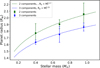 |
Fig. A.1 Comparison of the 2- and 3-component GMM fits for the radius valley values reveals that the inclusion of a third component improves the fit. |
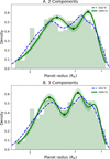 |
Fig. A.2 Comparison between the 2- and 3- component fit along with the KDE fits. It is clearly observed that the KDE fit goes along better with the 3- component GMM fit. |
Appendix B Confirmed and Candidate Planets
 |
Fig. B.1 We performed our GMM analysis on various planet samples, from top, all planet candidates and confirmed planets from our sample (A), planet candidates (B) and likely planets (C) obtained from our Triceratops run (Giacalone & Dressing 2020) and confirmed planets from the NASA exoplanet archive (D) with number of planets in parentheses. As it is shown, including the planet candidates not only increases the planet sample; it also helps to reduce the error bars on the peaks and minima and precisely locate the radius valley. |
References
- Ballard, S. 2019, AJ, 157, 113 [NASA ADS] [CrossRef] [Google Scholar]
- Barclay, T., Pepper, J., & Quintana, E. V. 2018, ApJS, 239, 2 [Google Scholar]
- Batalha, N. M., Borucki, W. J., Bryson, S. T., et al. 2011, AJ, 729, 27 [Google Scholar]
- Batalha, N. M., Rowe, J. F., Bryson, S. T., et al. 2013, ApJS, 204, 24 [Google Scholar]
- Berger, T. A., Huber, D., Gaidos, E., van Saders, J. L., & Weiss, L. M. 2020, AJ, 160, 108 [NASA ADS] [CrossRef] [Google Scholar]
- Berger, T. A., Schlieder, J. E., & Huber, D. 2023 arXiv preprint [arXiv:2302.00009] [Google Scholar]
- Bonfanti, A., Brady, M., Wilson, T. G., et al. 2023 A&A, 682, A66 [Google Scholar]
- Borucki, W. J., Koch, D., Basri, G., et al. 2010, Science, 327, 977 [Google Scholar]
- Cloutier, R., & Menou, K. 2020, AJ, 159, 211 [NASA ADS] [CrossRef] [Google Scholar]
- Dattilo, A., & Batalha, N. M. 2024, AJ, 167, 288 [Google Scholar]
- Dattilo, A., Batalha, N. M., & Bryson, S. 2023, AJ, 166, 122 [NASA ADS] [CrossRef] [Google Scholar]
- Dressing, C. D., & Charbonneau, D. 2013, AJ, 767, 95 [Google Scholar]
- Dressing, C. D., & Charbonneau, D. 2015, AJ, 807, 45 [Google Scholar]
- Fulton, B. J., Petigura, E. A., Howard, A. W., et al. 2017, AJ, 154, 109 [Google Scholar]
- Gaia Collaboration (Vallenari, A., et al.) 2023, A&A, 674, A1 [NASA ADS] [CrossRef] [EDP Sciences] [Google Scholar]
- Gaidos, E., Ali, A., Kraus, A. L., & Rowe, J. F. 2024 MNRAS, 534, 3277 [Google Scholar]
- Giacalone, S., & Dressing, C. D. 2020 triceratops: Candidate exoplanet rating tool, Astrophysics Source Code Library, [record ascl:2002.004] [Google Scholar]
- Giacalone, S., Dressing, C. D., Jensen, E. L. N., et al. 2021, AJ, 161, 24 [Google Scholar]
- Ginzburg, S., Schlichting, H. E., & Sari, R. 2018, MNRAS, 476, 759 [Google Scholar]
- Gupta, A., & Schlichting, H. E. 2019, MNRAS, 487, 24 [Google Scholar]
- Gupta, A., & Schlichting, H. E. 2020, MNRAS, 493, 792 [Google Scholar]
- Hardegree-Ullman, K. K., Apai, D., Bergsten, G. J., Pascucci, I., & López-Morales, M. 2023, AJ, 165, 267 [NASA ADS] [CrossRef] [Google Scholar]
- He, M. Y., Ford, E. B., & Ragozzine, D. 2019, MNRAS, 490, 4575 [CrossRef] [Google Scholar]
- Ho, C. S. K., & Van Eylen, V. 2023, MNRAS, 519, 4056 [NASA ADS] [CrossRef] [Google Scholar]
- Ho, C. S. K., Rogers, J. G., Van Eylen, V., Owen, J. E., & Schlichting, H. E. 2024, MNRAS, 531, 3698 [NASA ADS] [CrossRef] [Google Scholar]
- Howell, S. B., Sobeck, C., Haas, M., et al. 2014, PASP, 126, 398 [Google Scholar]
- Hsu, D. C., Ford, E. B., & Terrien, R. 2020, MNRAS, 498, 2249 [Google Scholar]
- Izidoro, A., Schlichting, H. E., Isella, A., et al. 2022, ApJ, 939, L19 [NASA ADS] [CrossRef] [Google Scholar]
- Lee, E. J., & Connors, N. J. 2021, ApJ, 908, 32 [NASA ADS] [CrossRef] [Google Scholar]
- Lee, E. J., Karalis, A., & Thorngren, D. P. 2022, AJ, 941, 186 [Google Scholar]
- Lindegren, L. 2018, gAIA-C3-TN-LU-LL-124 [Google Scholar]
- Lopez, E. D., & Rice, K. 2018, MNRAS, 479, 5303 [NASA ADS] [CrossRef] [Google Scholar]
- Luque, R., & Pallé, E. 2022, Science, 377, 1211 [NASA ADS] [CrossRef] [Google Scholar]
- Mulders, G. D., Pascucci, I., & Apai, D. 2015, AJ, 814, 130 [Google Scholar]
- Mulders, G. D., Pascucci, I., Apai, D., & Ciesla, F. J. 2018, AJ, 156, 24 [Google Scholar]
- Nielsen, J., Johansen, A., Bali, K., & Dorn, C. 2025, A&A, 695, A184 [NASA ADS] [CrossRef] [EDP Sciences] [Google Scholar]
- Owen, J. E., & Wu, Y. 2017, ApJ, 847, 29 [Google Scholar]
- Owen, J. E., & Murray-Clay, R. 2018, MNRAS, 480, 2206 [NASA ADS] [CrossRef] [Google Scholar]
- Parc, Bouchy, F., Venturini, J., Dorn, C., & Helled, R. 2024, A&A, 688, A59 [NASA ADS] [CrossRef] [EDP Sciences] [Google Scholar]
- Petigura, E. A., Howard, A. W., Marcy, G. W., et al. 2017, AJ, 154, 107 [NASA ADS] [CrossRef] [Google Scholar]
- Petigura, E. A., Rogers, J. G., Isaacson, H., et al. 2022, AJ, 163, 179 [NASA ADS] [CrossRef] [Google Scholar]
- Ricker, G. R., Winn, J. N., Vanderspek, R., et al. 2015, JATIS, 1, 014003 [Google Scholar]
- Rogers, L. A. 2015, AJ, 801, 41 [Google Scholar]
- Rogers, J. G., Gupta, A., Owen, J. E., & Schlichting, H. E. 2021, MNRAS, 508, 5886 [NASA ADS] [CrossRef] [Google Scholar]
- Stassun, K. G., Oelkers, R. J., Pepper, J., et al. 2018, AJ, 156, 102 [Google Scholar]
- Stassun, K. G., Oelkers, R. J., Paegert, M., et al. 2019, AJ, 158, 138 [Google Scholar]
- Tang, Y., Fortney, J. J., & Murray-Clay, R. 2024, ApJ, 976, 221 [Google Scholar]
- Thompson, S. E., Coughlin, J. L., Hoffman, K., et al. 2018, ApJS, 235, 38 [NASA ADS] [CrossRef] [Google Scholar]
- Venturini, Ronco, M. P., Guilera, O. M., et al. 2024, A&A, 686, L9 [NASA ADS] [CrossRef] [EDP Sciences] [Google Scholar]
- Wolfgang, A., Rogers, L. A., & Ford, E. B. 2016, ApJ, 825, 19 [Google Scholar]
- Wu, Y. 2019, AJ, 874, 91 [Google Scholar]
- Wyatt, M. C., Kral, Q., & Sinclair, C. A. 2019, MNRAS, 491, 782 [Google Scholar]
As on November 2, 2024.
All Tables
Super-Earth peaks, mini-Neptune peaks, and radius valley values from two- and three-component GMM fits for the entire sample and M, K, and G dwarfs.
All Figures
|
Fig. 1 Histogram comparing TESS objects of interest (TOIs) and Kepler objects of interest (KOIs) from the NASA Exoplanet Archive, with star counts indicated in parentheses. The inset plot (top left) highlights the significant increase in low-mass stars identified by TESS, which enhances our ability to study these stars in greater detail. |
| In the text | |
|
Fig. 2 Kernel density estimates along with the histograms of olanet radii distribution of the entire sample and M, K, G stellar types. |
| In the text | |
|
Fig. 3 GMM fits to the unbinned radius data, along with corresponding histograms, are presented for the entire low-mass star sample and for M, K, and G stellar types. The super-Earth and mini-Neptune peaks, as well as the radius valley, are indicated in each plot. |
| In the text | |
|
Fig. 4 Slope values, |
| In the text | |
|
Fig. 5 GMM fits along with their histograms for early and late M dwarfs. |
| In the text | |
|
Fig. 6 Comparison of our data with that of Wu (2019). The scaling from Wu is plotted with an offset for better alignment and easier comparison. |
| In the text | |
|
Fig. A.1 Comparison of the 2- and 3-component GMM fits for the radius valley values reveals that the inclusion of a third component improves the fit. |
| In the text | |
|
Fig. A.2 Comparison between the 2- and 3- component fit along with the KDE fits. It is clearly observed that the KDE fit goes along better with the 3- component GMM fit. |
| In the text | |
|
Fig. B.1 We performed our GMM analysis on various planet samples, from top, all planet candidates and confirmed planets from our sample (A), planet candidates (B) and likely planets (C) obtained from our Triceratops run (Giacalone & Dressing 2020) and confirmed planets from the NASA exoplanet archive (D) with number of planets in parentheses. As it is shown, including the planet candidates not only increases the planet sample; it also helps to reduce the error bars on the peaks and minima and precisely locate the radius valley. |
| In the text | |
Current usage metrics show cumulative count of Article Views (full-text article views including HTML views, PDF and ePub downloads, according to the available data) and Abstracts Views on Vision4Press platform.
Data correspond to usage on the plateform after 2015. The current usage metrics is available 48-96 hours after online publication and is updated daily on week days.
Initial download of the metrics may take a while.