| Issue |
A&A
Volume 703, November 2025
|
|
|---|---|---|
| Article Number | A302 | |
| Number of page(s) | 10 | |
| Section | Planets, planetary systems, and small bodies | |
| DOI | https://doi.org/10.1051/0004-6361/202554052 | |
| Published online | 26 November 2025 | |
Rotation periods of asteroids serendipitously observed by the NASA/Kepler K2 mission
1
Université Côte d’Azur, Observatoire de la Côte d’Azur,
CNRS, Laboratoire Lagrange,
France
2
V.N. Karazin Kharkiv National University,
Kharkiv,
Ukraine
3
Department of Aerospace Engineering, Grainger College of Engineering/Department of Astronomy/NCSA, University of Illinois at Urbana-Champaign,
Urbana,
IL 61801,
USA
4
IMCCE, Observatoire de Paris, PSL Research University, CNRS, Sorbonne Universités,
UPMC Univ Paris 06, Univ. Lille,
75014
Paris,
France
5
Aix Marseille Univ, CNRS, CNES, LAM, Laboratoire d’Astrophysique de Marseille,
Marseille,
France
★ Corresponding author: This email address is being protected from spambots. You need JavaScript enabled to view it.
Received:
6
February
2025
Accepted:
8
September
2025
Abstract
Context. Understanding the rotational periods of asteroids is crucial for gaining insights into their internal structures, compositions, and collisional histories. NASA’s Kepler Space Telescope, during its K2 extension (2014-2018), serendipitously observed numerous asteroids while surveying the ecliptic plane, providing a unique photometric dataset.
Aims. By analyzing photometric data from the K2 mission, we aimed to determine the rotational periods of asteroids that crossed Kepler’s field of view, focusing on objects with an apparent magnitude of 19 or brighter that appeared in the Kepler target pixel files at least ten times.
Methods. We developed an algorithm to identify asteroid crossings in the Kepler data and extract photometric light curves. The Lomb–Scargle periodogram method was employed to determine the rotational periods from the extracted light curves due to its robustness in handling unevenly sampled data. Noise and systematic errors were mitigated through photometric corrections using co-trending basis vectors.
Results. We extracted and analyzed 4,596 light curves from 2,418 asteroids observed during the Kepler/K2 mission. This allowed us to compute rotation periods for 559 asteroids. We found that 375 of these asteroids had previously known periods. The rotation periods determined for 295 of the asteroids in this study agree with existing asteroid rotation periods from the literature, validating our approach. We report new rotation periods and their light curve amplitudes for 184 asteroids, expanding the catalog of known asteroid rotation periods.
Conclusions. The analysis of rotation periods from the Kepler K2 mission data has provided valuable insights into the physical characteristics of main-belt asteroids. Our results are consistent with existing data and expand the catalog of known asteroid rotation periods. These findings contribute to our understanding of asteroid dynamics and will aid future research in planetary science and asteroid exploration.
Key words: methods: data analysis / techniques: photometric / surveys / minor planets, asteroids: general
© The Authors 2025
 Open Access article, published by EDP Sciences, under the terms of the Creative Commons Attribution License (https://creativecommons.org/licenses/by/4.0), which permits unrestricted use, distribution, and reproduction in any medium, provided the original work is properly cited.
This article is published in open access under the Subscribe to Open model. This email address is being protected from spambots. You need JavaScript enabled to view it. to support open access publication.
1 Introduction
The Kepler Space Telescope, launched by NASA in 2009, was initially designed to detect Earth-like planets orbiting other stars by monitoring changes in their brightness (Borucki et al. 2009). After the completion of its primary mission, Kepler embarked on a second phase, known as the K2 mission. The K2 mission, initiated after two of Kepler’s four reaction wheels failed, adapted the spacecraft’s operations to observe different parts of the ecliptic plane during campaigns of approximately 80 days (Howell et al. 2014). This new mode not only extended the life of the mission but also broadened its scientific scope to include more varied objects and phenomena within the Solar System, including asteroids (Szabó et al. 2015; Berthier et al. 2016; Kalup et al. 2021).
The observation of asteroids with Kepler, particularly during the K2 phase, presented a unique opportunity. Unlike groundbased telescopes, Kepler’s extended observation periods along the ecliptic, where most asteroids reside, enabled continuous and precise photometric data collection. As remnants of the early Solar System, asteroids are particularly compelling study subjects. They offer insights into the primitive materials and conditions that existed during its formation (Morbidelli et al. 2015). Studying the rotational periods and surface properties of asteroids can provide crucial information about their structural integrity and evolutionary trajectories, which are vital for understanding potential impact hazards and for future asteroid space mission initiatives (Athanasopoulos et al. 2024; Novaković et al. 2022; Oszkiewicz et al. 2023; Pravec et al. 2008).
Leveraging the unique capabilities of the K2 mission, this research capitalizes on the serendipitous observations of asteroids that transited Kepler’s field of view (FOV). Specifically, we aimed to extract precise photometric data, estimate rotational periods, and conduct a comprehensive analysis of the physical characteristics of these asteroids. Such efforts contribute significant insights to the planetary sciences community, complementing existing asteroid catalogs and enhancing our overall understanding of these minor bodies.
In the subsequent sections, we delve into the methodologies used for photometric extraction from the Kepler data, describe the analytical techniques for estimating rotation periods, and discuss the broader implications of our findings against the backdrop of current asteroid research. The extended capabilities of the Kepler spacecraft, particularly during the K2 mission, underscore the benefits of continuous, space-based observation platforms for minor body research in the Solar System.
In Sect. 2, we present the data collection and preparation methods. In Sect. 3, we explain the prediction of asteroid signals and the computation of asteroid crossings. In Sect. 4 we discuss the magnitude and FOV limits that influence detection capabilities. We outline the process of light curve extraction in Sect. 5 and rotation period estimation in Sect. 6, and we present our results in Sect. 7.
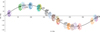 |
Fig. 1 Locations of the Kepler K2 mission fields of view along with their campaign numbers (c0 through c20). The black line indicates the ecliptic plane. |
2 Data
The process of extracting photometry from Kepler data involves several essential steps, starting with acquiring the appropriate datasets. The Kepler K2 mission was conducted in a series of sequential “Campaigns” with observing fields distributed along the ecliptic plane. A total of 21 campaigns were successfully completed between 2014 and 2018, each lasting around 80 days (see Fig. 1).
The raw data, available from the Mikulski Archive for Space Telescopes (MAST), consist of target pixel files (TPFs) for each campaign. During a typical K2 campaign, the mission collected approximately 15 000−30 000 TPFs, each corresponding to an individual target. The exact number of TPFs varied based on the campaign’s specific scientific objectives, the stellar density of the field being observed, and the prioritization of high-interest targets.
The TPFs contain time-series data representing the flux received from each pixel associated with a specific Kepler target, including transient objects crossing the FOV. They hold uncalibrated pixel data, which are processed later to correct for instrumental effects, cosmic ray impacts, and background noise. Each TPF includes metadata such as target coordinates, observing cadence mode, pixel array dimensions, and timestamps for each frame. The typical TPFs contain pixel arrays ranging from 5×5 to 15×15 pixels per timestamp, ensuring precise spatial coverage while observing a target and the nearby background.
Kepler utilized two observational cadence modes: long cadence (29.4 minutes) and short cadence (1 minute). Long cadence was predominantly employed, facilitating the capture of gradual variability over extended periods while balancing data storage and processing requirements. During each of the 80-day campaigns, the long cadence mode targeted between 15 000 and 20 000 objects, yielding approximately 3900 data points per target. Short cadence mode, on the other hand, targeted between 50 and 100 objects per campaign, providing higher temporal resolution to address specific scientific inquiries, such as stellar oscillations and rapid astrophysical phenomena.
3 Prediction of asteroid crossings
Identifying asteroids in the Kepler data is a crucial step in the analysis pipeline. The primary challenge is distinguishing asteroids from other transient signals, such as cosmic rays, background stars, and instrumental artifacts. Due to technical issues causing minor movement of the target fields of view, photometric measurements of any existing object in the Kepler TPF are quite challenging. As a result, we did not analyze images for random events but focused on studying known asteroids that could be identified through their ephemerides.
To this end, we employed Algorithm 1 to calculate the path of asteroids that would cross target boxes in the Kepler FOV. An example of such an asteroid crossing is presented in Fig. 2. We extracted ephemerides of known Solar System objects (SSOs) as seen from the Kepler spacecraft via SkyBoT (Berthier et al. 2006; Berthier et al. 2016). This step returned objects that fell within a slightly extended Kepler FOV, accounting for the proper motion of the SSOs during long exposures. Another coarse filtering step with respect to the distance of each SSO to the Kepler Input Catalog (KIC) and Ecliptic Plane Input Catalog (EPIC) box centers at every observation epoch was used to eliminate objects that were not observed. The paths of remaining objects that would likely cross a KIC/EPIC box were translated into Kepler pixel positions as a function of time.
The output of Algorithm 1 contained a list of candidate SSO/KIC object encounters. Qualitatively, those encounters can be categorized as (a) incomplete or too few observations, where the object only grazes the box, (b) below detection limit, where the object was too faint to be detected or below the S/N cutoff described in Sect. 4, and (c) close enough and bright enough to have a noticeable impact on the photometric time-series in the box. We only considered objects of these “Close Encounters of the Third Kind” (c) in this analysis.
By processing the entire Kepler K2 dataset with this algorithm, we identified 1,308,311 asteroid crossings involving 46,708 unique asteroids across the 21 campaigns. Figure 3 shows the distribution of asteroids crossing predicted over the entire K2 mission.
 |
Fig. 2 Crossing of the asteroid Eunomia by the Kepler K2 field number EPIC 202685494 in September 2014. The aperture mask of the target star is marked by red squares. |
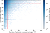 |
Fig. 3 Distribution of asteroids predicted to cross during the K2 observation campaign. The dashed red lines indicate the constraints on the processed asteroid observations: the horizontal line at magnitude 19 marks the cutoff above which asteroids are considered “too faint” to be reliably detected, while the vertical line marks the threshold below which there are “too few observations” of an asteroid per TPF. |
4 Magnitude and field of view limits
The magnitude limit of the Kepler K2 mission’s long cadence images depended on the target’s brightness and observing conditions, which varied across different campaigns due to changes in stellar density, background noise, and specific scientific priorities. Target selection was optimized for detecting exoplanet transits around stars with 8 ≤ Kp ≤ 16 magnitude range (Batalha et al. 2010). However, Kepler K2 could observe stars down to a faint limit of approximately 20−21 magnitude in the Kp band (Ridden-Harper et al. 2020). For stars at 12th magnitude, Kepler achieved a photometric precision better than 170 parts per million, while for stars at the 18th magnitude, the precision was around 0.01 mag, and for stars at 20th magnitude, it was 0.1 mag. The limiting magnitude was influenced by factors such as crowding and background noise, with source confusion being the primary limiting factor for fainter sources (Szabó et al. 2016).
1: Input: Kepler spacecraft (s/c) ephemeris file, SkyBoT based asteroid ephemeris file with respect to Kepler s/c, mid-exposure time file, EPIC box coordinates file.
2: Output: FOV crossing information for each asteroid within each Kepler target box.
3: Initialize variables: Read configuration values, such as mid-exposure times, ephemeris data, and box coordinates.
4: Compute the Kepler FOV direction vector in the International Celestial Reference Frame (ICRF).
5: Load ephemeris data:
6: For each asteroid in the ephemeris file do
7: Interpolate asteroid positions and velocities for mid-exposure times using spline interpolation.
8: end for
9: Read EPIC box information:
10: for each EPIC target box do
11: Transform box center and corner coordinates into RA and Dec, considering the pixel scale and rotation matrix.
12: end for
13: Determine FOV crossings:
14: for each mid-exposure time do
15: for each EPIC box do
16: Compute the distance vector of the asteroid’s position relative to the box center.
17: Check if the asteroid lies within the box boundaries, accounting for the box orientation and size.
18: if the asteroid crosses the FOV then
19: Compute the barycentric Julian date (BJD) correction for the FOV offset.
20: Output the crossing information, including pixel location, velocity, and BJD correction.
21: end if
22: end for
23: end for
24: Output results: Save asteroid ID and FOV crossing details such as EPIC box position/pixel as a function of time.
The observed asteroid sample was largely composed of faint objects, many with magnitudes fainter than 20. Here, we focused on processing asteroids with apparent magnitudes of 19 and brighter to ensure reliable detection above the background noise. The number of asteroids detected per campaign varied based on observing conditions such as sky brightness, crowding, and the position of the asteroid within the FOV. Of the asteroids observed, approximately 15 000 distinct asteroids brighter than magnitude 19 were followed up by Kepler K2 more than 150 000 times (Fig. 3).
The Kepler K2 mission’s TPF FOV is constrained to a specific area of the sky, which varies depending on the observed target due to changes in pointing direction and the position of the target within the spacecraft’s viewing area. Given the Kepler detector’s pixel size of 3.98 arcsec, the FOV typically ranges from 20 to 60 arcsec, encompassing the target star and its surrounding background. This limited FOV presents challenges when observing transient objects like asteroids, as they can move significantly during the observation period.
The restricted FOV, combined with the typical proper motion of main belt asteroids (approximately 30 arcsec per hour), limits our ability to determine long spin periods for asteroids. As a result, we focused on analyzing asteroids that appeared in the individual FOV of the Kepler TPFs at least ten times, which allowed us to cover half of the spin period range for most known asteroids.
We focused on asteroids with more than ten observations and apparent magnitudes brighter than 19. This threshold was chosen to ensure that the asteroids were sufficiently bright for reliable photometric measurements, which are essential for estimating their spin periods. Although most asteroids did not satisfy these selection criteria, we successfully identified more than 4,596 observations corresponding to 2,418 distinct asteroids, from which we extracted their light curves.
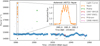 |
Fig. 4 Light curve of the TPF 201686550 obtained from the Kepler K2 mission. The colored markers indicate predicted asteroid crossings. |
5 Light curve extraction
Kepler’s point spread function (PSF) varies across the FOV depending on the position of the target star. The PSF’s diameter ranges from 3.1 to 7.5 arcsec, with a median value of 4.2 arcsec. Despite this variability, the PSF remains relatively stable within each TPF.
Light curve extraction techniques are generally optimized for stationary targets like stars. This process typically involves summing the flux from all pixels within the target’s aperture, followed by background subtraction and corrections for systematic effects (Smith et al. 2012). The main challenge arises when dealing with moving targets, which can introduce systematic errors into the photometry. In Kepler’s case, this motion is caused by both spacecraft jitter and the movement of asteroids. As a result, standard photometric techniques used for star observation often perform poorly when applied to asteroids crossing small fields of view, particularly when a bright source is also present.
To address these challenges, we tested various techniques for extracting light curve photometry and found that the most effective approach was to estimate the sum of the flux from all pixels within the TPF. Since asteroids often move through multiple apertures, summing the entire TPF ensured that we captured the object’s flux consistently despite its motion.
After summing the flux, we applied corrections to the obtained light curve using co-trending basis vectors (CBVs). CBVs are a key component of the Kepler data processing pipeline designed to remove a variety of instrumental systematics, including those caused by spacecraft motion, instrument temperature variations, and detector effects. CBVs are derived from a large dataset of Kepler observations using principal component analysis. Each observation quarter has its own set of CBV parameters, which includes 84 extensions (corresponding to each CCD channel) and 16 basis vectors per channel (Smith et al. 2020).
This technique provided an optimal signal-to-noise ratio while minimizing the impact of background noise and instrumental artifacts. An example of a light curve obtained using this approach for TPF 201686550 is shown in Fig. 4, with predicted asteroid crossings highlighted by colored markers.
Once the light curves were extracted, they were normalized to the median flux of the target to correct for systematic variations in the data. This normalization reduced errors that might distort the asteroid’s light curve, leading to a more accurate assessment of its properties. We then cropped the light curves to cover the asteroid crossing event, along with a few hours before and after the crossing to estimate the local background. We used background fluctuations to estimate the uncertainty of the provided data, as the main source of noise in the obtained asteroid light curves is the Poisson noise of the target and surrounding stellar objects.
The final processing of the asteroid light curves involved fitting and removing the trapezoidal signal from the data. This step was necessary to estimate the apparent magnitude of the asteroid and to correct for signals at the edge of the TPF. The trapezoidal signal was fitted to the light curve using a least-squares optimization algorithm, and the resulting fit was subtracted from the light curve. The corrected light curve was then used to estimate the rotation period of the asteroid. The resulting light curve change of an asteroid crossing is shown in Fig. 5.
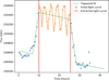 |
Fig. 5 Light curve change of asteroid 6427 (1995 FY) crossing TPF number 212160907. The trapezoidal signal fit is shown by the dotted green line. The vertical red lines indicate the asteroid processing window. |
6 Rotation period estimation
The rotation period of an asteroid is a crucial property that offers valuable insights into its physical characteristics, including shape, size, and surface properties. This period can be estimated by examining the periodic variations in the asteroid’s light curve, which occur due to its rotation around its axis. A widely used method for determining the rotation period from discrete measurements is the Lomb–Scargle periodogram, a robust tool for detecting periodic signals in unevenly sampled time-series data (Lomb 1976; Scargle 1982).
We used the PyAstronomy package (Czesla et al. 2019) for the implementation of the generalized Lomb–Scargle (GLS) periodogram (Zechmeister & Kürster 2009; Ferraz-Mello 1981), which fits the trigonometric function to account for measurement uncertainties and a constant term. This package allowed us to compute the periodogram for each asteroid’s light curve and identify the most likely rotation period based on the peak of the periodogram. We limited the search range to frequencies corresponding to rotation periods between 2 hours and the Nyquist frequency of the light curve. This range ensured that we captured the majority of the asteroid’s rotation periods while considering the number of data points in the light curve.
To compute the Lomb–Scargle periodogram, we used the measured light curves as well as the estimated uncertainties of the data. The uncertainties of the edge points were adjusted by a factor depending on their distance from the edge, resulting in more accurate periodogram results.
For any time series of measurements (ti, yi) where i = 1, 2, …, N is associated with a standard deviation (σi), and the weights  , we aimed to minimize the weighted sum of squared residuals:
![Mathematical equation: $V_{\text {res}}=\chi^{2}(\omega)=\sum_{i=1}^{N} w_{i}\left[y_{i}-A \cos \left(\omega t_{i}\right)-B \sin \left(\omega t_{i}\right)-C\right]^{2},$](/articles/aa/full_html/2025/11/aa54052-25/aa54052-25-eq2.png)
where A, B, and C are the parameters of the model. The LombScargle periodogram power at frequency ω is defined as the fraction of variance explained by the sinusoidal model:

where Vy is the total weighted variance of the data. The periodogram power is a measure of the significance of the periodic signal at a given frequency. The peak of the periodogram indicates the most likely rotation period of the asteroid.
To determine whether a signal contains a periodic component and to assess the significance of the periodogram peak, we calculated the false alarm probability (FAP). The FAP quantifies the likelihood that a peak in the periodogram of a noisy dataset (with no real periodic signal) exceeds a certain power purely by chance. In the context of the GLS periodogram with weighted data and a constant term, computing the FAP involves understanding the statistical distribution of the periodogram’s power under the null hypothesis (i.e., no periodic signal).
For the GLS, the test statistic, Θ, can be defined based on the ratio of variances:

where N is the number of data points, M is the number of fitted parameters (M=3 for A, B and C), Vmodel=Vy−Vres is the variance explained by the model at frequency ω, Vy is the total weighted variance of the data, and Vres is the residual variance after fitting the model.
The single-frequency (or per-frequency) FAP is given by

where v1 = 2 M and v2 = 2(N−M) are the degrees of freedom, and FΘ is the cumulative distribution function of the F-distribution.
Since we scanned over multiple frequencies, we had a higher probability of observing a high power by chance. To account for this, we adjusted the FAP:
![Mathematical equation: $\mathrm{FAP}=1-\left[1-\operatorname{FAP}_{\text {single}}(\omega)\right]^{N_{\text {ind}}},$](/articles/aa/full_html/2025/11/aa54052-25/aa54052-25-eq6.png)
where Nind is the number of independent frequencies tested. The number of independent frequencies is estimated as Nind=N/2, where N is the number of data points in the light curve.
For each asteroid in our catalog, we provide the significance level of the periodogram peak, which indicates the reliability of the detected rotation period. We provide a peak significance level for each asteroid in the final catalog. An example of the periodogram analysis result for the asteroid (23788) Cofer light curve is presented in Fig. 6.
As asteroids cross the full frame image field, they can be observed multiple times as they move through different TPFs. For 177 asteroids that re-entered the Kepler K2 FOV on multiple times, we obtained repeated observations in the form of multiple light curves. In this case, we computed the periodograms for each light curve individually and then averaged them to obtain a more accurate estimate of the rotation period.
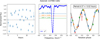 |
Fig. 6 Left: light curve of asteroid (23788) Cofer extracted from the Kepler K2 mission data. Middle: Lomb–Scargle periodogram, with horizontal dotted lines indicating the FAP significance levels. Right: folded light curve. Colored points indicate the phase of the observed light curve. |
7 Results
Out of the 2,418 processed asteroids, we determined rotation periods for only 559. This is a result of a combination of factors, including an insufficient number of observations for a given asteroid’s spin period, high noise levels in the data, and low intrinsic variability amplitudes. For clarity, we define two hierarchical working samples that are used consistently throughout this article:
Initial sample: The 2,418 asteroids brighter than Kp = 19 that were observed by the Kepler K2 mission at least ten times. This represents the complete set of asteroids processed in this work. Within this initial set, 1,145 asteroids already had a rotation period published in the literature;
Kepler-period sample: The 559 asteroids from the initial sample for which we obtained a reliable rotation period. This is the main catalog presented here. To be included, a period determination required a periodogram peak significance above 95% (FAP < 0.05) and a period uncertainty of less than 20% of the estimated value. This sample includes 375 asteroids with previously published periods and 184 new periods determined in this work.
Our findings reveal that most of the periods determined in this work lie in the range of ∼2−24 hours, which is biased due to observation conditions and the limited number of observations. Specifically, the requirement of having at least 10 observations in a campaign means that asteroids with very long rotation periods (comparable to or exceeding the campaign duration) are unlikely to be detected, and our magnitude cutoff (Kp = 19) favors asteroids with sufficient brightness and variability. These selection effects skew our sample toward faster rotators (Marciniak et al. 2015).
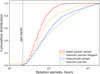 |
Fig. 7 Cumulative distributions of the rotation periods for the initial sample (blue line), Kepler-period sample (red line), SsODNet reference catalog (green line), and flagged sample (orange line). The vertical dashed line indicates the 2.2-hour spin barrier. |
7.1 Comparison with known periods
To compare the Kepler-period sample with previously published rotation periods, we used the Solar System Open Database Network (SsODNet; Berthier et al. 2023), which consolidates data from multiple sources such as the Lightcurve Database (LCDB; Warner et al. 2021). SsODNet provides the most reliable estimates of rotation periods and includes quality flags, which we used to validate our results.
Figure 7 compares the cumulative distribution functions of rotation periods across these four datasets. The SsODNet reference catalog (green) serves as our reference population, comprising over 50 000 asteroids and reaching its median value near P ≈ 30 h. The initial sample (blue) shows a distribution that is almost similar to the SsODNet distribution. The flagged sample (orange) contains 6840 periods that have been assigned LCDB quality codes U=2 ± or 3 ±. Finally, the Kepler-period sample (red) is dominated by rapid rotators, with 50% spin in less than 6 hours and 80% in less than 15 hours. The dashed lines mark the well-known 2.2-hour “spin barrier” (see Pravec et al. 2002, for instance), which is the limit for asteroid rotation periods.
In the LCDB, a quality flag of U ≥ 2 is only assigned when a low-scatter light curve spans at least one complete rotation and yields a unique period solution (see Warner et al. 2021). For ground-based telescopes, interruptions due to the diurnal gap make such continuous coverage practically impossible, so high U determinations are inherently biased toward faster rotators. We therefore believe that the clear excess of asteroids that rotate very quickly in the Kepler-period sample and the flagged sample is due to observational cadence and duty-cycle selection effects, and not because the distribution of asteroid spin rates is genuinely different.
To assess the reliability of our period determinations, we compared our results for 375 asteroids from the Kepler-period sample with previously published values in the SsODNet (see Fig. 8). We find a strong correlation between the two datasets, with 80% of the asteroids showing agreement within the 3 σ uncertainty range. The reliability of our measurements is further underscored when examining a high-quality subset of 58 asteroids, which have a quality flag of U=3 in the LCDB. For this group, the agreement level increases to around 85%. However, it is important to note that, due to observational constraints such as the magnitude cutoff and the minimum number of required observations, our Kepler-period sample is biased toward faster-rotating asteroids.
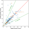 |
Fig. 8 Comparison of rotation periods derived from Kepler K2 observations with those reported in the SsODNet. Blue points represent asteroids with known periods but without quality flags, while orange points indicate asteroids with a quality flag of U=3. The dashed red line indicates a 1:1 agreement between Kepler and comparison periods, while the dashed green lines represent half and twice the Kepler period. Error bars reflect uncertainties in the period determinations, where available. |
7.2 Rotation periods and asteroid taxonomy
We also explored the relationship between rotational periods and asteroid taxonomy. For this analysis, we focused on the asteroids in our Kepler-period sample that have published taxonomic classifications, as an illustration of the presently released dataset. Among these, the vast majority belong to three broad types: C-type (carbonaceous), S-type (silicaceous), and X-type asteroids. We therefore limited our taxonomic comparison to the subset of 336 asteroids with known classifications of these three broad types, which are the most common in the main asteroid belt.
Specifically, we analyzed the rotation period distribution for the dominant asteroid types: C-type (carbonaceous), S-type (silicaceous), and X-type asteroids (Mahlke et al. 2022). Figure 9 illustrates that S-type asteroids tend to have shorter rotation periods compared to C-type asteroids. The X-type asteroids, which are a mixture of E, M, and P types of asteroids, exhibit intermediate rotation periods.
We quantified the relative abundance of C and S types as a function of rotation period (or equivalently, density constraint) by computing the fraction C/(C + S) in different regimes of the dotted lines in Fig. 9. The relative fraction of C-type asteroids decreases from about 40% for the lowest-density regime (corresponding to very slow rotators, right side of the figure) to 29% for densities between 0.5 and 1 g/cm3 (middle part of the figure), and to 23% for the highest-density regime (left side of the figure). This trend could be attributed to differences in their internal structures and compositions. S-type asteroids, being rockier and denser, may have more cohesive structures, which would enable them to rotate faster without breaking apart (Zhang et al. 2022). In contrast, C-type asteroids are generally less dense and more porous, making them more likely to rotate slowly without disruptive centrifugal forces. These findings are consistent with previous studies that suggest a correlation between asteroid composition and rotational dynamics. Our results in that context serve to validate that our newly derived rotation periods align with established physical patterns.
However, we were surprised to find that the C-type asteroids (31416) Peteworden and (25454) 1999 XN12 appear among the fast-rotators in the left part of Fig. 9. Both asteroids exhibit rotation periods of approximately 2.5 hours and light curve amplitudes of about 0.4 magnitudes. The Zwicky Transient Facility (ZTF) data confirm our findings: analysis of its sparse observations yielded consistent rotation periods and amplitudes, in good agreement with the values previously observed by Kepler K2. Additionally, color analysis – particularly the g-r and i-z indices supports their classification as primarily C types, with X type as the second most probable complex (Sergeyev et al. 2022). Taken together, these factors suggest that these asteroids have a metallic composition. This finding highlights the value of combining data from multiple sources to improve our understanding of asteroid taxonomy and composition.
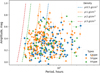 |
Fig. 9 Distribution of the rotation period of the asteroids with taxonomy. The dotted lines represent the density constraints derived from the equilibrium between gravitational acceleration at the surface and centrifugal acceleration at the equator. Colored markers indicate the asteroid types: C (carbonaceous), S (silicaceous), and X (a mixture of E, M, and P types). |
8 Conclusion
We have analyzed photometric data from the NASA Kepler/K2 mission, determining rotation periods for a sample of 559 mainbelt asteroids, of which 184 are new discoveries. To validate our methodology, we compared our results with previously published values in SsODNet. We find a good correspondence between the datasets, with the periods for approximately 80% of the 375 asteroids common to both samples in agreement. This provides confidence in the reliability of our results, including the newly determined periods.
Our analysis confirms that the serendipitous observations from the K2 mission are a valuable resource for asteroid science. The sample is subject to an observational bias favoring the detection of objects with periods shorter than 24 hours.
We detected distinct patterns that reflect differences in composition and internal structure by correlating the derived rotation periods with each asteroid’s known taxonomy. Our analysis confirms that denser, silicate-rich S-type asteroids tend to have, on average, shorter rotation periods than the less dense, carbonaceous C-type asteroids. This trend supports the idea that rockier and more cohesive bodies can sustain faster spins, while more porous objects have slower rotations due to their lower material strength.
Our dataset revealed a few notable outliers. For example, some asteroids classified as C types were found to rotate unusually fast, with periods of around 2.5 hours and moderate light curve amplitudes, which suggests that these objects have atypically high densities. A more detailed analysis indicated that these asteroids were likely misclassified and probably belong to the metal-rich X-type complex. These cases highlight the importance of combining different data sources, such as continuous light curves, sparse ground-based observations like those provided by ZTF (Carry et al. 2024), upcoming LSST data, and spectral and color measurements, to improve asteroid classification and gain a deeper understanding of their physical properties.
Data availability
The table listing each object’s rotation period, light-curve amplitude, and other parameters is available at the CDS via https://cdsarc.cds.unistra.fr/viz-bin/cat/J/A+A/703/A302
Acknowledgements
S.E. acknowledges support from the National Science Foundation through Collaborative Research: Rubin Rocks: Enabling near-Earth asteroid science with LSST NSF Award Number: 2307570. A.V.S. acknowledges support from the Agence Nationale de la Recherche (ANR) and the PAUSE program for refugees through ANR-PAUSE funding. This research was supported by the International Research Travel Award Program-Ukraine (APS IRTAPU-kraine) of the American Physical Society, with funding provided by the Alfred P. Sloan Foundation. The properties of Solar System objects were retrieved using the rocks1 python client of the SsODNet Virtual Observatory (VO) Web service2 (Berthier et al. 2023). This research used the IMCCE’s Miriade3 VO Web service (Berthier et al. 2009) and TOPCAT4 VO client (Taylor 2005). Thanks to all the developers and maintainers.
References
- Albers, K., Kragh, K., Monnier, A., et al. 2010, Minor Planet Bull., 37, 152 [Google Scholar]
- Antonini, P., Behrend, R., Colas, F., et al. 2011, Central Bureau Electron. Telegrams, 2698, 1 [Google Scholar]
- Athanasopoulos, D., Hanuš, J., Avdellidou, C., et al. 2024, in European Planetary Science Congress, EPSC2024–359 [Google Scholar]
- Aznar Macias, A., 2016, Minor Planet Bull., 43, 350 [Google Scholar]
- Batalha, N. M., Borucki, W. J., Koch, D. G., et al. 2010, ApJ, 713, L109 [NASA ADS] [CrossRef] [Google Scholar]
- Berthier, J., Vachier, F., Thuillot, W., et al. 2006, in Astronomical Society of the Pacific Conference Series, 351, Astronomical Data Analysis Software and Systems XV, eds. C. Gabriel, C. Arviset, D. Ponz, & S. Enrique, 367 [Google Scholar]
- Berthier, J., Hestroffer, D., Carry, B., et al. 2009, in European Planetary Science Congress 2009, 676 [Google Scholar]
- Berthier, J., Carry, B., Vachier, F., Eggl, S., & Santerne, A., 2016, MNRAS, 458, 3394 [NASA ADS] [CrossRef] [Google Scholar]
- Berthier, J., Carry, B., Mahlke, M., & Normand, J., 2023, A&A, 671, A151 [NASA ADS] [CrossRef] [EDP Sciences] [Google Scholar]
- Borucki, W. J., Koch, D., Jenkins, J., et al. 2009, Science, 325, 709 [Google Scholar]
- Carry, B., Peloton, J., Le Montagner, R., Mahlke, M., & Berthier, J., 2024, A&A, 687, A38 [NASA ADS] [CrossRef] [EDP Sciences] [Google Scholar]
- Cellino, A., Tanga, P., Muinonen, K., & Mignard, F., 2024, A&A, 687, A277 [NASA ADS] [CrossRef] [EDP Sciences] [Google Scholar]
- Chang, C.-K., Ip, W.-H., Lin, H.-W.,, et al. 2014, ApJ, 788, 17 [NASA ADS] [CrossRef] [Google Scholar]
- Chang, C.-K., Ip, W.-H., Lin, H.-W.,, et al. 2015, ApJS, 219, 27 [NASA ADS] [CrossRef] [Google Scholar]
- Chang, C.-K., Lin, H.-W., Ip, W.-H.,, et al. 2016, ApJS, 227, 20 [Google Scholar]
- Chang, C.-K., Lin, H.-W., Ip, W.-H.,, et al. 2019, ApJS, 241, 6 [Google Scholar]
- Childers, D., & Church, A., 2007, Minor Planet Bull., 34, 124 [Google Scholar]
- Chiorny, V. G., Shevchenko, V. G., Slyusarev, I. G., et al. 2023, Planet. Space Sci., 237, 105779 [Google Scholar]
- Clark, M., 2019, Minor Planet Bull., 46, 346 [Google Scholar]
- Cordwell, A. J., Rattenbury, N. J., Bannister, M. T., et al. 2022, MNRAS, 514, 3098 [Google Scholar]
- Czesla, S., Schröter, S., Schneider, C. P., et al. 2019, PyA: Python astronomy-related packages, Astrophysics Source Code Library [record ascl:1906.010] [Google Scholar]
- Davies, M. E., Colvin, T. R., Belton, M. J. S., Veverka, J., & Thomas, P. C., 1996, Icarus, 120, 33 [Google Scholar]
- Ditteon, R., Black, S., Masner, Z., Osborne, J., & Trent, L., 2018, Minor Planet Bull., 45, 338 [Google Scholar]
- Durech, J., Kaasalainen, M., Warner, B. D., et al. 2009, A&A, 493, 291 [NASA ADS] [CrossRef] [EDP Sciences] [Google Scholar]
- Ďurech, J., & Hanuš, J., 2023, A&A, 675, A24 [NASA ADS] [CrossRef] [EDP Sciences] [Google Scholar]
- Ďurech, J., Hanuš, J., Oszkiewicz, D., & Vančo, R., 2016, A&A, 587, A48 [NASA ADS] [CrossRef] [EDP Sciences] [Google Scholar]
- Ďurech, J., Hanuš, J., & Alí-Lagoa, V., 2018, A&A, 617, A57 [NASA ADS] [CrossRef] [EDP Sciences] [Google Scholar]
- Durech, J., Tonry, J., Erasmus, N., et al. 2020, A&A, 643, A59 [NASA ADS] [CrossRef] [EDP Sciences] [Google Scholar]
- Ďurech, J., Vávra, M., Vančo, R., & Erasmus, N., 2022, Front. Astron. Space Sci., 9, 809771 [Google Scholar]
- Ferraz-Mello, S., 1981, AJ, 86, 619 [NASA ADS] [CrossRef] [Google Scholar]
- Ferrero, A., 2012, Minor Planet Bull., 39, 65 [Google Scholar]
- French, L. M., Stephens, R. D., Lederer, S. M., Coley, D. R., & Rohl, D. A., 2011, Minor Planet Bull., 38, 116 [Google Scholar]
- French, L. M., Stephens, R. D., Coley, D. R., Megna, R., & Wasserman, L. H., 2012, Minor Planet Bull., 39, 183 [Google Scholar]
- French, L. M., Stephens, D. R., Coley, D. R.,, et al. 2013, Minor Planet Bull., 40, 198 [Google Scholar]
- Galad, A., 2008, Minor Planet Bull., 35, 17 [Google Scholar]
- Hanuš, J., Ďurech, J., Oszkiewicz, D. A., et al. 2016, A&A, 586, A108 [NASA ADS] [CrossRef] [EDP Sciences] [Google Scholar]
- Hanuš, J., Delbo’, M., Alí-Lagoa, V., et al. 2018, Icarus, 299, 84 [CrossRef] [Google Scholar]
- Harris, A. W., Young, J. W., Dockweiler, T., et al. 1992, Icarus, 95, 115 [NASA ADS] [CrossRef] [Google Scholar]
- Howell, S. B., Sobeck, C., Haas, M., et al. 2014, PASP, 126, 398 [Google Scholar]
- Husárik, M., 2018, Contrib. Astron. Observ. Skalnate Pleso, 48, 319 [Google Scholar]
- Kalup, C. E., Molnár, L., Kiss, C., et al. 2021, ApJS, 254, 7 [NASA ADS] [CrossRef] [Google Scholar]
- Licchelli, D., 2006, Minor Planet Bull., 33, 50 [Google Scholar]
- Lomb, N. R., 1976, Ap&SS, 39, 447 [Google Scholar]
- Mahlke, M., Carry, B., & Mattei, P. A., 2022, A&A, 665, A26 [NASA ADS] [CrossRef] [EDP Sciences] [Google Scholar]
- Marciniak, A., Pilcher, F., Oszkiewicz, D., et al. 2015, Planet. Space Sci., 118, 256 [NASA ADS] [CrossRef] [Google Scholar]
- Marciniak, A., Alí-Lagoa, V., Müller, T. G., et al. 2019, A&A, 625, A139 [NASA ADS] [CrossRef] [EDP Sciences] [Google Scholar]
- Marciniak, A., Durech, J., Alí-Lagoa, V., et al. 2021, A&A, 654, A87 [NASA ADS] [CrossRef] [EDP Sciences] [Google Scholar]
- Martikainen, J., Muinonen, K., Penttilä, A., Cellino, A., & Wang, X. B., 2021, A&A, 649, A98 [NASA ADS] [CrossRef] [EDP Sciences] [Google Scholar]
- Masiero, J., Jedicke, R., Ďurech, J., et al. 2009, Icarus, 204, 145 [Google Scholar]
- McNeill, A., Mommert, M., Trilling, D. E., Llama, J., & Skiff, B., 2019, ApJS, 245, 29 [Google Scholar]
- McNeill, A., Gowanlock, M., Mommert, M., et al. 2023, AJ, 166, 152 [NASA ADS] [CrossRef] [Google Scholar]
- Morbidelli, A., Walsh, K. J., O’Brien, D. P., Minton, D. A., & Bottke, W. F., 2015, The Dynamical Evolution of the Asteroid Belt, 493 [Google Scholar]
- Mottola, S., Di Martino, M., Erikson, A., et al. 2011, AJ, 141, 170 [Google Scholar]
- Novaković, B., Vokrouhlický, D., Spoto, F., & Nesvorný, D., 2022, Celest. Mech. Dyn. Astron., 134, 34 [NASA ADS] [CrossRef] [Google Scholar]
- Oey, J., 2009, Minor Planet Bull., 36, 4 [NASA ADS] [Google Scholar]
- Oszkiewicz, D., Troianskyi, V., Galád, A., et al. 2023, Icarus, 397, 115520 [NASA ADS] [CrossRef] [Google Scholar]
- Pravec, P., Harris, A. W., & Michalowski, T., 2002, Asteroids III, 113 [Google Scholar]
- Pravec, P., Harris, A. W., Vokrouhlický, D., et al. 2008, Icarus, 197, 497 [NASA ADS] [CrossRef] [Google Scholar]
- Pray, D. P., Galad, A., Husarik, M., & Oey, J., 2008, Minor Planet Bull., 35, 34 [Google Scholar]
- Ridden-Harper, R., Tucker, B. E., Gully-Santiago, M., et al. 2020, MNRAS, 498, 33 [Google Scholar]
- Ryan, E. L., Sharkey, B. N. L., & Woodward, C. E., 2017, AJ, 153, 116 [NASA ADS] [CrossRef] [Google Scholar]
- Scargle, J. D., 1982, ApJ, 263, 835 [Google Scholar]
- Sergeyev, A. V., Carry, B., Onken, C. A., et al. 2022, A&A, 658, A109 [NASA ADS] [CrossRef] [EDP Sciences] [Google Scholar]
- Shevchenko, V. G., Belskaya, I. N., Slyusarev, I. G., et al. 2012, Icarus, 217, 202 [NASA ADS] [CrossRef] [Google Scholar]
- Simpson, G., Chong, E., Gerhardt, M., et al. 2013, Minor Planet Bull., 40, 146 [Google Scholar]
- Skiff, B. A., McLelland, K. P., Sanborn, J. J., Pravec, P., & Koehn, B. W., 2019, Minor Planet Bull., 46, 458 [Google Scholar]
- Slivan, S. M., Binzel, R. P., Crespo da Silva, L. D., et al. 2003, Icarus, 162, 285 [Google Scholar]
- Smith, J. C., Stumpe, M. C., Van Cleve, J. E., et al. 2012, PASP, 124, 1000 [Google Scholar]
- Smith, J. C., Stumpe, M. C., Jenkins, J. M., et al. 2020, Kepler Data Processing Handbook: Presearch Data Conditioning, Kepler Science Document KSCI-19081-003, 8, ed. J. M. Jenkins [Google Scholar]
- Stephens, R. D. 2012a, Minor Planet Bull., 39, 11 [Google Scholar]
- Stephens, R. D. 2012b, Minor Planet Bull., 39, 80 [Google Scholar]
- Stephens, R. D., & Warner, B. D., 2018, Minor Planet Bull., 45, 48 [Google Scholar]
- Stephens, R. D., & Warner, B. D. 2019a, Minor Planet Bull., 46, 73 [Google Scholar]
- Stephens, R. D., & Warner, B. D. 2019b, Minor Planet Bull., 46, 449 [Google Scholar]
- Szabó, R., Sárneczky, K., Szabó, G. M., et al. 2015, AJ, 149, 112 [Google Scholar]
- Szabó, R., Pál, A., Sárneczky, K., et al. 2016, A&A, 596, A40 [NASA ADS] [CrossRef] [EDP Sciences] [Google Scholar]
- Szabó, G. M., Pál, A., Kiss, C., et al. 2017, A&A, 599, A44 [NASA ADS] [CrossRef] [EDP Sciences] [Google Scholar]
- Tan, H., Yeh, T., Li, B., & Gao, X., 2018, Minor Planet Bull., 45, 57 [NASA ADS] [Google Scholar]
- Taylor, M. B., 2005, in Astronomical Society of the Pacific Conference Series, 347, Astronomical Data Analysis Software and Systems XIV, eds. P. Shopbell, M. Britton, & R. Ebert, 29 [Google Scholar]
- Vernazza, P., Ferrais, M., Jorda, L., et al. 2021, A&A, 654, A56 [NASA ADS] [CrossRef] [EDP Sciences] [Google Scholar]
- Warner, B. D., 2006, Minor Planet Bull., 33, 39 [Google Scholar]
- Warner, B. D., 2008, Minor Planet Bull., 35, 95 [Google Scholar]
- Warner, B. D., 2019, Minor Planet Bull., 46, 46 [Google Scholar]
- Warner, B. D., & Stephens, R. D., 2019, Minor Planet Bull., 46, 161 [Google Scholar]
- Warner, B. D., & Stephens, R. D., 2020, Minor Planet Bull., 47, 37 [Google Scholar]
- Warner, B. D., & Stephens, R. D., 2021, Minor Planet Bull., 48, 40 [Google Scholar]
- Warner, B. D., Aznar Macias, A., Benishek, V., Oey, J., & Gross, R., 2017, Minor Planet Bull., 44, 325 [Google Scholar]
- Warner, B. D., Stephens, R. D., & Coley, D. R., 2018, Minor Planet Bull., 45, 147 [Google Scholar]
- Warner, B. D., Harris, A. W., & Pravec, P., 2021, Asteroid Lightcurve Database (LCDB) Bundle V4.0, NASA Planetary Data System, urn:nasa:pds:ast-lightcurve-database::4.0 [Google Scholar]
- Waszczak, A., Chang, C.-K., Ofek, E. O., et al. 2015, AJ, 150, 75 [NASA ADS] [CrossRef] [Google Scholar]
- Yeh, T.-S., Li, B., Chang, C., et al.-K., 2020, AJ, 160, 73 [NASA ADS] [CrossRef] [Google Scholar]
- Zechmeister, M., & Kürster, M., 2009, A&A, 496, 577 [CrossRef] [EDP Sciences] [Google Scholar]
- Zhang, Y., Michel, P., Barnouin, O. S., et al. 2022, Nat. Commun., 13, 4589 [NASA ADS] [CrossRef] [Google Scholar]
Appendix A Asteroid table description
The asteroids table contains various parameters describing the physical and orbital properties of asteroids. Below is a brief description of the columns included in the table:
Name - Provisional or official designation of the asteroid.
Number - Official asteroid number assigned by the Minor Planet Center.
Period - Measured rotation period of the asteroid (in hours).
Period err - Uncertainty in the measured rotation period.
FAP - False alarm probability of the detected period.
Mag var. - Observed variation in brightness (magnitude).
Mag var. err. - Uncertainty in the brightness variation.
Dyn class - Dynamical classification of the asteroid (e.g., Main Belt, Mars-Crosser).
Taxonomy - Spectral classification of the asteroid.
Table A.1 presents the few first rows of the dataset.
Example entries from the asteroid table.
Appendix B Sources referenced for known asteroid rotation periods
Harris et al. (1992); Davies et al. (1996); Slivan et al. (2003); Warner (2006); Licchelli (2006); Childers & Church (2007); Galad (2008); Pray et al. (2008); Warner (2008); Durech et al. (2009); Masiero et al. (2009); Oey (2009); Albers et al. (2010); Mottola et al. (2011); Antonini et al. (2011); French et al. (2011); Shevchenko et al. (2012); Stephens (2012a); Ferrero (2012); Stephens (2012b); French et al. (2012); Simpson et al. (2013); French et al. (2013); Chang et al. (2014); Waszczak et al. (2015); Chang et al. (2015); Hanuš et al. (2016); Ďurech et al. (2016); Chang et al. (2016); Aznar Macias (2016); Szabó et al. (2017); Ryan et al. (2017); Warner et al. (2017); Ďurech et al. (2018); Husárik (2018); Hanuš et al. (2018); Stephens & Warner (2018); Tan et al. (2018); Warner et al. (2018); Ditteon et al. (2018); Marciniak et al. (2019); Chang et al. (2019); McNeill et al. (2019); Warner (2019); Stephens & Warner (2019a); Warner & Stephens (2019); Clark (2019); Stephens & Warner (2019b); Skiff et al. (2019); Ďurech et al. (2020); Yeh et al. (2020); Warner & Stephens (2020); Martikainen et al. (2021); Vernazza et al. (2021); Marciniak et al. (2021); Warner & Stephens (2021); Ďurech et al. (2022); Cordwell et al. (2022); Ďurech & Hanuš (2023); McNeill et al. (2023); Oszkiewicz et al. (2023); Chiorny et al. (2023); Cellino et al. (2024)
All Tables
All Figures
|
Fig. 1 Locations of the Kepler K2 mission fields of view along with their campaign numbers (c0 through c20). The black line indicates the ecliptic plane. |
| In the text | |
|
Fig. 2 Crossing of the asteroid Eunomia by the Kepler K2 field number EPIC 202685494 in September 2014. The aperture mask of the target star is marked by red squares. |
| In the text | |
|
Fig. 3 Distribution of asteroids predicted to cross during the K2 observation campaign. The dashed red lines indicate the constraints on the processed asteroid observations: the horizontal line at magnitude 19 marks the cutoff above which asteroids are considered “too faint” to be reliably detected, while the vertical line marks the threshold below which there are “too few observations” of an asteroid per TPF. |
| In the text | |
|
Fig. 4 Light curve of the TPF 201686550 obtained from the Kepler K2 mission. The colored markers indicate predicted asteroid crossings. |
| In the text | |
|
Fig. 5 Light curve change of asteroid 6427 (1995 FY) crossing TPF number 212160907. The trapezoidal signal fit is shown by the dotted green line. The vertical red lines indicate the asteroid processing window. |
| In the text | |
|
Fig. 6 Left: light curve of asteroid (23788) Cofer extracted from the Kepler K2 mission data. Middle: Lomb–Scargle periodogram, with horizontal dotted lines indicating the FAP significance levels. Right: folded light curve. Colored points indicate the phase of the observed light curve. |
| In the text | |
|
Fig. 7 Cumulative distributions of the rotation periods for the initial sample (blue line), Kepler-period sample (red line), SsODNet reference catalog (green line), and flagged sample (orange line). The vertical dashed line indicates the 2.2-hour spin barrier. |
| In the text | |
|
Fig. 8 Comparison of rotation periods derived from Kepler K2 observations with those reported in the SsODNet. Blue points represent asteroids with known periods but without quality flags, while orange points indicate asteroids with a quality flag of U=3. The dashed red line indicates a 1:1 agreement between Kepler and comparison periods, while the dashed green lines represent half and twice the Kepler period. Error bars reflect uncertainties in the period determinations, where available. |
| In the text | |
|
Fig. 9 Distribution of the rotation period of the asteroids with taxonomy. The dotted lines represent the density constraints derived from the equilibrium between gravitational acceleration at the surface and centrifugal acceleration at the equator. Colored markers indicate the asteroid types: C (carbonaceous), S (silicaceous), and X (a mixture of E, M, and P types). |
| In the text | |
Current usage metrics show cumulative count of Article Views (full-text article views including HTML views, PDF and ePub downloads, according to the available data) and Abstracts Views on Vision4Press platform.
Data correspond to usage on the plateform after 2015. The current usage metrics is available 48-96 hours after online publication and is updated daily on week days.
Initial download of the metrics may take a while.