| Issue |
A&A
Volume 703, November 2025
|
|
|---|---|---|
| Article Number | A299 | |
| Number of page(s) | 9 | |
| Section | Stellar structure and evolution | |
| DOI | https://doi.org/10.1051/0004-6361/202555257 | |
| Published online | 26 November 2025 | |
Magnetar-like flares behind the high-energy emission in LS 5039
1
Departament de Física Quàntica i Astrofísica, Institut de Ciències del Cosmos, Universitat de Barcelona, IEEC-UB, Martí i Franquès 1, 08028 Barcelona, Spain
2
Institute of Astronomy, Russian Academy of Sciences, Moscow 119017, Russia
⋆ Corresponding authors: This email address is being protected from spambots. You need JavaScript enabled to view it.
; This email address is being protected from spambots. You need JavaScript enabled to view it.
Received:
22
April
2025
Accepted:
19
October
2025
Abstract
Context. LS 5039 is a system hosting a high-mass star and a compact object of unclear nature. There are hints that the system may host a strongly magnetized neutron star, a scenario that requires a mechanism to power its persistent and strong nonthermal emission.
Aims. We investigate a mechanism in which the nonsteady interaction structure of the stellar and the compact object winds can regularly excite neutron star magnetospheric activity, which can release extra energy and fuel the source nonthermal emission.
Methods. The neutron star wind shocked by the stellar wind can recurrently touch the neutron star magnetosphere, triggering magnetic instabilities whose growth can release extra energy into the neutron star wind in a cyclic manner. To illustrate and study the impact of these cycles on the two-wind interaction structure on different scales, we performed relativistic hydrodynamics simulations in two and three dimensions with periods of an enhanced power in the neutron star wind along the orbit. We also used analytical tools to characterize processes near the neutron star relevant for the nonthermal emission.
Results. As the neutron star wind termination shock touches the magnetosphere energy dissipation occurs, but the whole shocked two-wind structure is eventually driven away, stopping the extra energy injection. However, due to the corresponding drop in the neutron star wind ram pressure, the termination shock propagates back toward the magnetosphere, resuming the process. These cycles of activity excite strong waves in the shocked flows, intensifying their mixing and the disruption of their spiral-like structure produced by orbital motion. Further downstream, the shocked winds can become a quasi-stable, relatively smooth flow.
Conclusions. The recurrent interaction between the neutron star magnetosphere and a shocked wind can fuel a relativistic outflow powerful enough to explain the nonthermal emission of LS 5039. A magnetospheric multipolar magnetic field much stronger than the dipolar one may provide the required energetics, and help to explain the lack of evidence of a recent supernova remnant.
Key words: hydrodynamics / radiation mechanisms: non-thermal / stars: magnetars / stars: winds / outflows / X-rays: binaries
© The Authors 2025
 Open Access article, published by EDP Sciences, under the terms of the Creative Commons Attribution License (https://creativecommons.org/licenses/by/4.0), which permits unrestricted use, distribution, and reproduction in any medium, provided the original work is properly cited.
This article is published in open access under the Subscribe to Open model. This email address is being protected from spambots. You need JavaScript enabled to view it. to support open access publication.
1. Introduction
LS 5039 is a binary system hosting an O6.5 V star and a compact object of unclear origin (Casares et al. 2005), and a powerful gamma-ray source with a nonthermal radiation luminosity, LNT ∼ 1036 erg s−1, peaking around ∼10 − 100 MeV (e.g., Collmar & Zhang 2014). As was shown in Casares et al. (2005), a black hole in the system is likely only if the latter is pseudo-synchronized, although hints of P ≈ 9 s period pulsations found in X-rays would favor a pulsar if confirmed (Yoneda et al. 2020). Despite evidence of X-ray pulsations being under debate (Kargaltsev et al. 2023; Makishima et al. 2023), they would strongly indicate the presence of a slowly rotating, magnetar-like neutron star (NS), make the standard scenario of a pulsar in the ejector regime less likely due to a low wind power, and favor a magnetospheric origin for the energy fueling the nonthermal emission (Yoneda et al. 2020). It is worth noting that LS I +61 303, a similar high-mass binary and gamma-ray emitter, has been found to host a relatively slowly rotating NS that may also present magnetar-like behavior (e.g., Weng et al. 2022, and references therein). Given all this, a model for energizing the nonthermal emitter with the energy stored in the NS magnetosphere may be required in these sources.
Yoneda et al. (2020) explored analytically the possibility of feeding the nonthermal emission in LS 5039 with energy from the magnetosphere, released due to its interaction with the stellar wind, but the specifics of this interaction were not provided. Moreover, the presence of a magnetar in the system should be reconciled with the absence of evidence for a very young supernova remnant (SNR) near LS 5039 (Moldón et al. 2012). Magnetar flares have been discussed in the literature (see, e.g., Beloborodov 2020; Khangulyan et al. 2022, and references therein) as the sources of fast radio bursts (FRBs; Lorimer et al. 2007), particularly in the context of flares of a magnetar in a high-mass binary (Bozzo et al. 2008) when there is periodicity (see, e.g., Lyutikov et al. 2020b; Barkov & Popov 2022), so LS 5039 hosting a magnetar would fit in this framework. Thus, in this work we propose a mechanism for LS 5039 based on recurrent periods of magnetar-like flaring activity. These periods start with a weak NS (or pulsar) wind that cannot balance the ram pressure of the wind from the companion star, and the shocked pulsar wind can reach or even enter the light cylinder of the NS, directly touching its magnetosphere (as is proposed in Yoneda et al. 2020). This can trigger magnetic perturbations in the magnetosphere that can quickly grow, and ultimately lead to magnetic reconnection and the release of large amounts of energy into the otherwise weak pulsar wind beyond the light cylinder (Barkov et al. 2022; Sharma et al. 2023). The injection of magnetospheric energy lasts as long as the pulsar wind termination shock touches the magnetosphere, and during this period the shocked pulsar wind mediates the energy transfer between the latter (i.e., the energy source) and the region resulting from the star-pulsar wind interaction (i.e., where -or downstream of which- the nonthermal emitter is located). Eventually, though, the enhanced pulsar wind drives the whole shocked flow structure beyond the light cylinder, stopping the injection of energy. This severely reduces the pulsar wind ram pressure and the shocked pulsar wind quickly expands inward until it again touches the magnetosphere, moment at which the cycle can repeat. This process leads to recurrent periods of power-enhanced pulsar wind that feed the overall nonthermal emission in the system. To show how the shocked structure evolves, we carried out relativistic hydrodynamics (RHD) simulations that mimic the effect of the magnetic active periods on the shocked winds, including the role of orbital motion. We also explored, using analytical tools, the processes near the NS relevant for the nonthermal emission.
Regular pulsar winds (i.e., not enhanced by magnetar activity) can already be significantly magnetized and nonspherically symmetric (e.g., Bogovalov et al. 2019). Moreover, the part of the wind enhanced by magnetar activity can also cover a relatively narrow solid angle of a few steradians, which increases the wind anisotropy (Sharma et al. 2023). In addition, three-dimensional (3D) relativistic magnetohydrodynamics (RMHD) simulations (Porth et al. 2014; Barkov et al. 2024) showed that the shocked pulsar wind structure is very sensitive to changes in the environment. Thus, the magnetic field is indeed a major factor in the problem, and should eventually be included in simulations of the discussed scenario. However, the 3D RMHD solution turned out to be on average similar to that for a spherical RHD wind, which also shows strong instabilities (see sect. 3 in Barkov et al. 2024). Furthermore, the simulations presented here took about 100 000 CPU hours; since an RMHD simulation requires at least a 10 times higher spatial resolution, the computational time should be ∼109 CPU hours, which is extremely hard to achieve. For all this, at this stage RHD simulations were employed as they provide qualitatively relevant results, while keeping the computing costs at a reasonable level and allowing for an exploratory study.
The article is structured as follows: In Sect. 2 the simulations are described, and their results are shown in Sect. 3. Then, in Sect. 4, a discussion is carried out about the regime of interaction between the NS and the surrounding medium, the origin of the nonthermal energy and the age of the system, and the nonthermal emitter.
2. Simulation setup
The RHD simulations were performed in 2D and 3D geometry in Cartesian (2D and 3D) and cylindrical (axisymmetric 2D) coordinates using the PLUTO code1 (Mignone et al. 2007). Spatial linear interpolation, a third-order Runge-Kutta approximation in time, and an HLLC Riemann solver were adopted (Li 2005). PLUTO is a modular Godunov-type code entirely written in C and intended mainly for astrophysical applications and high-Mach-number flows in multiple spatial dimensions. The simulations were performed on the CFCA XC50 cluster of the National Astronomical Observatory of Japan (NAOJ) and RIKEN HOKUSAI Bigwaterfall. The flow was approximated as an ideal, relativistic adiabatic gas, with one particle species and a polytropic index of 4/3. The size of the Cartesian domain is x and y ∈ [ − 32, 32] in 2D and 3D, and z ∈ [ − 20, 20] in 3D. The resolution is nonuniform in the entire computational domain, with a total number of cells: NX = NY = 780 (2D and 3D), and NZ = 650 (3D; see details in Table 1). The size of the axisymmetric domain is r ∈ [0, 0.7], and z ∈ [0.7, 2.0], with a total number of cells: Nr = 260, and NZ = 360. The higher-resolution central part features Nr = 130, and NZ = 260, with size r ∈ [0, 0.25], and z ∈ [0.7, 1.2].
In this paper, the unit of length a = 2.2 × 1012 cm corresponds to the semimajor axis for an orbital period of Torb ≈ 3.9 days and a binary total mass of ≈30 M⊙ (Casares et al. 2005). This work was intended as a first exploration of the phenomenon under study. Thus, the results of the Cartesian 2D simulations were meant to be illustrative of the large-scale evolution (Bosch-Ramon et al. 2012), but the difficulty in capturing in detail the magnetospheric scale (∼10−2 times smaller than a; see Sect. 4) precluded in that case a detailed characterization of the shocked pulsar wind evolution right between the star and the NS. The latter limitation also affects the Cartesian 3D simulations. Nevertheless, the tendencies in the flow evolution on the smallest captured scales hinted at the role of the shocked pulsar wind when enhanced by strong magnetospheric activity. In the Cartesian simulations, a corresponds to ≈64 cells. On the other hand, the axisymmetric 2D simulations allowed us to study the shocked two-wind region closest to the magnetosphere, with a corresponding now to ≈520 cells, but without including orbital motion, the latter playing a minor role on those scales. Finally, the equation of state adopted, albeit simple, is already enough to derive meaningful conclusions from the simulations (see the explorations carried out in Bosch-Ramon et al. 2012, 2015; Barkov et al. 2024).
2.1. Setup of the winds
The wind of the massive star is assumed to be cold and move radially with constant velocity vw = 2400 km/s and Mach number Mw = 7. The pulsar wind is also cold and moves radially with Lorentz factor Γpw = 1.9 and Mach number Mpw = 17, and the star-to-pulsar wind momentum rate ratio is η = 0.05 in the weak wind phase in the Cartesian simulations and η = 4 × 10⁻⁴ in the axisymmetric simulations, where
 (1)
(1)
with Ėsd being the spin-down power of the pulsar and Ṁ the massive star mass-loss rate. The winds were modeled similarly to those in Bosch-Ramon et al. (2015). During flaring periods, in the Cartesian case η grows such that its orbit-averaged value reaches 0.16, but in one case it reaches 0.39 (in the axisymmetric case only one flare is presented; see the next section).
2.2. Setup of the magnetar flaring periods
The flaring periods were approximated via a function representing recurrent additional injections of power, Ėpw ∝ Ėfl(1+δρ) ∝ ρpw(1+δρ), which has the following time profile:
 (2)
(2)
where  is a dimensionless time variable normalized to the orbital period, Torb, ρpw is the weak pulsar wind density, Nfl the number of flaring periods per orbit, Δ the relative width of the flaring period, and Afl its amplitude. The last two terms quantify how much energy per orbit is released by the flaring periods compared to the one from the weak pulsar wind alone, Torb < Ėfl > and Torb < Ėsd >, respectively2. The time profile of the flaring periods was chosen to be sharp, while avoiding numerical artifacts in the simulations. A profile with Δ = 0.1 is presented in Fig. 1 for better visualization, but in the simulations a narrower profile with Δ = 0.05 was used. In the Cartesian simulations, the energy injection averaged over the orbit including both the flaring and weak wind periods releases 3.3 (≡ < η > = 0.16) and 7.8 (≡ < η > = 0.39) times more energy than the weak pulsar wind alone (η = 0.05). The maximum enhancement of injected power within the flaring periods is higher: 72 (max(ηfl) = 3.6) and 214 (max(ηfl) = 10.7) times larger than in the weak wind phase. The parameter values used are presented in Table 2. In the axisymmetric simulations, we were exploring a different spatial and temporal scale, as was allowed by the more focused setup, and the flare was made significantly shorter to mimic the response of the shocked structure on the scales of the magnetospheric radius. Thus we took Δ = 0.003, and the adopted maximum enhancement of injected power during the flaring period was higher, by a factor of 870, which corresponds to max(ηfl) = 0.35 from η = 4 × 10⁻⁴.
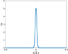 |
Fig. 1. Example of the time profile of a flaring period; δρ is the density on top of the regular pulsar wind density during flaring periods, x = 2πtNfl/Torb the dimensionless time (see Sect. 2.1 for details), and Δ = 0.1 the width of the pulse. |
Parameters of the Cartesian models.
3. Results
We carried out simulations for four 2D models and one 3D model in Cartesian coordinates including orbital motion, and one simulation for one 2D axisymmetric model. In the 2D Cartesian models, we varied the number of flaring periods during the orbit (Nfl = 10, 30, 90) for an orbit-averaged power of the flaring component alone of < Ėfl > = 2.3 < Ėsd >, and for Nfl = 30, we varied the flaring period power ×3 (i.e., < Ėfl > = 6.8 < Ėsd >). For higher flaring period rates, the interaction structure becomes smoother. In the case 2Dn90e10, with Nfl = 90, the leading edge of the shock is the most uniform (see Fig. 2, left top panel). The result of multiple flaring periods can be seen most clearly in the radial shock fronts that form on the trailing side of the interaction structure. Non-flare solutions are also shown, nfeta0.05 and nfeta0.5, which illustrate two cases with a strong difference in η, 0.05 (weak wind) and 0.5 (enhanced wind), but without the effect of the flaring periods (left and right bottom panels in Fig. 2). The main differences between the flare and non-flare solutions are: 1) the free pulsar wind zone (FPWZ), which is significantly smaller in the cases with flares, and 2) the spiral tail is significantly more loaded by the stellar wind in those cases. Point 2 is best illustrated by comparing the density of the shocked pulsar wind in the cases with flares and those without. Due to heavy mass-loading, the shocked pulsar wind in the spiral arm is slower in the cases with flares.
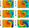 |
Fig. 2. Colored density maps on the orbital plane, with colored arrows representing the modulus of the 3-velocity vector for the 2D models. The flaring period rates are Nf = 90 (top left, 2Dn90e10), 30 (top right, 2Dn30e10), and 10 (middle left, 2Dn10e10) flaring periods per orbit, keeping the total energy budget of the system constant. In the model 2Dn30e30, we increased the power of the flaring period by a factor of 3, while keeping Nf = 30 (middle right panel). The non-flaring cases are presented at the bottom left (nfeta0.05) and right (nfeta0.5). |
For the cases 2Dn30e10 and 2Dn10e10, the individual flaring periods are more powerful and more separated in time compared to 2Dn90e10 (top right, middle left, and middle right panels in Fig. 2, respectively). As a result, the impacts of individual flaring periods become clearly visible in the density structure of both the leading and the trailing sides of the interaction structure. Increasing the orbit-averaged flaring period power, as seen comparing the 2Dn30e10 and the 2Dn30e30 models (top right and middle right panels in Fig. 2, respectively), leads to a larger two-wind interaction structure, while the FPWZ size decreases when increasing this power.
In the 3D simulations (model 3Dn30e10; Fig. 3), we switched on the flaring periods for short periods of time in a series of five flaring periods to mimic the flaring period impact within a fraction of the orbit (they occur for one sixth of the orbit), as the higher computational demands in 3D prevented us from probing the effect of the recurrent flaring periods for as long a time as in 2D. As we know from previous work (see, e.g., Bosch-Ramon et al. 2015), the results in 3D are more turbulent than in 2D in general, so the flares enhance turbulence further. The impact of the flaring periods on the overall two-wind interaction structure can be better seen in Fig. 4, although the limitations of the simulations prevented us from reproducing in detail the evolution of the pulsar wind termination shock; this is exemplified by a zoom-in of the interaction structure for the 3D simulations shown in Fig. 5, where the pulsar wind termination shock does not actually reach the magnetospheric scales. On the other hand, in the 2D axisymmetric simulations presented in Fig. 6, which do not account for orbital motion but probe more realistically the spatial and temporal scales close to the NS, the cycle of weak-enhanced-weak pulsar wind was better captured. The series of events that the simulations show can be described as follows. Initially, the magnetospheric flares are not active, and the weak pulsar wind termination shock can reach close to the NS, mimicking the situation when this shock is about to touch the magnetosphere (Fig. 6, top left3). When this happens, the flaring period resumes (Fig. 6, top right). Due to its high density, the shocked stellar wind reacts slowly to the power-enhanced pulsar wind and the shocked pulsar wind stays in contact with the magnetosphere, still exciting the magnetospheric activity for some time (Fig. 6, middle left). Eventually, as the shocked stellar wind is pushed outward, the pulsar wind termination shock moves away from the magnetosphere, and the extra energy injection stops (Fig. 6, middle right). At that point, the weakening of the pulsar wind allows the shocked pulsar wind to quickly propagate inward, toward the magnetosphere (Fig. 6, bottom panels), the system again becoming ready to restart the cycle. Using 2D axisymmetric simulations on small scales more systematically to better inform simulations on large scales (which here deal in a simplified manner with those small scales) is to be tackled in future studies.
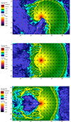 |
Fig. 3. Colored density maps with colored arrows representing the modulus of the 3-velocity vector for the 3D model (3Dn30e10) for various cuts: XY (top; orbital plane), XZ (middle), and ZY (bottom). |
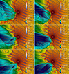 |
Fig. 4. Colored density maps with colored arrows representing the modulus of the 3-velocity vector for the 3D model (3Dn30e10) for cuts on the orbital plane, at orbital phases ϕ = 0.5435 (top left), ϕ = 0.575 (top right), ϕ = 0.5812 (middle left), ϕ = 0.6033 (middle right), ϕ = 0.6467 (bottom left), and ϕ = 0.6576 (bottom right). |
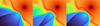 |
Fig. 5. Zoom-in of three snapshots of the cycle followed by the interaction structure: weak pulsar wind (left), enhanced pulsar wind (middle), and the end of energy injection (right). |
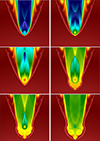 |
Fig. 6. Colored density maps obtained from an axisymmetric simulation showing qualitatively the evolution of a flare, from top left to bottom right: 0 (weak wind), 48 (flare starts), 88 (flare continuation), 141 (end of flare), 166 (pulsar wind approaches magnetosphere), and 186 s (flare about to resume) from the beginning of the flare. The grid size is ≈0.65 a; the magnetosphere radius would be ≈0.02 a in this case. |
4. Summary and discussion
In the previous section, we described how magnetospheric energy can be recurrently injected in the two-wind interaction region, and we illustrated this process with RHD simulations. Some caveats were raised in Sect. 1, as the pulsar wind enhanced by magnetar flares is expected to be magnetized and not spherically symmetric (e.g., Sharma et al. 2023). However, these differences from a spherical RHD wind are alleviated by the fact that other common factors (stellar wind, the nonsteady nature of the shocked flows, orbital motion, etc.) also play a strong role in the evolution of the interaction structure. Moreover, strong relativistic waves are expected between the magnetosphere and the stellar wind during magnetar flares, which can lead to a more spherical shocked pulsar wind, and to a reduction in the wind magnetization. Assessing all this requires detailed future analysis, and better connecting processes taking place on different spatial and temporal scales. Putting these caveats aside, in what follows some aspects of the proposed scenario are discussed; namely, the regime in which the stellar wind interacts with the NS surroundings, the nonthermal energy origin and the age of the source, the latter being relevant as no recent SNR has been found near LS 5039. The article finishes with a few remarks regarding the nonthermal emitter. In all the expressions below, we adopted the convention Aξ = A/10ξ, with A being in cgs units but for Ṁ, which is in units of solar masses per year.
4.1. NS-medium interaction regime
A NS interacting with a stellar wind can have two regimes in LS 5039: (1) ejector and (2) georotator (or propeller; see below; Illarionov & Syunyayev 1975; Lipunov 1992), which are discussed below. The state of the system is characterized by several radii: The distance at which pulsar and stellar winds would be in ram pressure balance4:
 (3)
(3)
the light cylinder radius,
 (4)
(4)
the Alfvenic radius at the balance location between the stellar wind ram pressure and the dipolar magnetic pressure of the NS magnetosphere:
 (5)
(5)
where μ = BdpRNS3 is the dipolar NS magnetic moment, and Bdp the dipolar magnetic field at the NS surface; and the gravitational capture radius:
 (6)
(6)
for MNS = 1.4 M⊙ and a wind speed normalization close to, but a bit lower than, its velocity at infinity of ≈2.4 × 108 cm s−1 (Casares et al. 2005), as we took into account the compactness of the system. For Bdp ≳ 4 × 10¹³ G (and taking RNS = 106 cm), one has Rg < RA, which is the reason we focus on the georotator regime hereafter. Nevertheless, the propeller regime could still be compatible with the triggering of magnetic flares. We did not account for a multipolar magnetic field (see below) when deriving RA as such a field drops much faster than Bdp.
The induced magnetospheric flares could be possible either in a marginal ejector regime, or in the georotator regime. Let us discuss first the ejector regime.
4.1.1. Ejector regime
The ejector regime takes place if Rs > RLC. From the dipole formula, the spin-down power becomes
 (7)
(7)
where Ω = 2π/P. For simplicity, in Eq. (7) we neglected the dependence on the angle between between the magnetic momentum and the rotation axis, which is ∼(1 + sin(α)2) (see, for numerical force-free simulations, e.g., Bogovalov 1999; Spitkovsky 2006, and for the analytical expression (2/3)sin(α)2, e.g., the review by Beskin 2010), and we simplified it to ∼1, but it does not change our conclusions significantly. The marginal ejector regime would correspond then to Rs temporarily reaching RLC. Taking Rs = RLC, one can derive a minimum dipolar magnetic field for the ejector regime:
 (8)
(8)
where we assumed η ≪ 1. In the marginal ejector regime, the magnetospheric flares would occur when Bdp ∼ Bcr. If Bdp = Bcr, the dipole spin-down time would be
 (9)
(9)
where I ≈ 1045 g cm2 is the NS moment of inertia.
The Tsd value obtained assuming Bdp = Bcr is similar to the τ ∼ 500 yr inferred from the X-ray data by Yoneda et al. (2020) and Makishima et al. (2023) for the pulsar spin-down. Under the same assumption, the spin-down power, Ėsd, is ∼7 × 1034 erg s−1, which is also close to the value inferred by Yoneda et al. (2020), and significantly below LNT ∼ 1036 erg s−1 in LS 5039. This spin-down power would correspond to the weak pulsar wind phase in the simulations, that is, between flaring periods. We recall that in the Cartesian simulations including orbital motion, η = 0.05 was adopted due to resolution limitations, making the simulation results qualitative, and in reality η would be much smaller, as in the axisymmetric simulation. For Ėsd ∼ 7 × 1034 erg s−1, Ṁ ∼ 4 × 10⁻⁷ M⊙ yr−1, and vw ∼ 2 × 108 cm s−1, one obtains η ∼ 5 × 10⁻⁴.
4.1.2. Georotator regime
For Bdp < Bcr, which implies that Rs < RLC, the system is in the georotator regime and the stellar wind directly interacts with the NS magnetosphere, and the maximum spin-down power associated with this interaction can be derived as follows. First, the mass rate of the stellar wind intercepted by the NS magnetosphere is obtained:
 (10)
(10)
which, following (Lyutikov et al. 2020a), allows for the maximum power dissipated on the magnetosphere boundary to be derived, as the incoming flow is forced to corotate with the NS magnetic field5:
 (11)
(11)
This value is similar to the Ėsd value obtained above, so the small amount of energy released in this regime when no flares happen may also be considered equivalent to the weak pulsar wind phase in the simulations.
From the maximum power estimate given in Eq. (11), in the georotator regime the spin-down time is
 (12)
(12)
Taking Tsd, Gr = τ ∼ 500 yr from Yoneda et al. (2020), one can estimate the minimum dipolar NS magnetic moment as (τ units are seconds: 500 yr ≈1010.2 s)
 (13)
(13)
so the minimum dipolar NS magnetic field is
 (14)
(14)
Adopting Bdp = Bcr, Rg is ∼0.3 RA for the source specific parameters, whereas taking Bdp = Bdp, min, Rg becomes ∼0.8RA, still marginally in the georotator regime. Importantly, the lower value of Bdp in the latter case can lead to a much longer ejector phase; for μ = μmin,
 (15)
(15)
where P has been normalized now to 2 s to account for pulsar rotation braking while still fulfilling Rs > RLC (ejector). If one sets Bcr = Bdp, min, one can obtain the longest pulsar period for which this condition is still fulfilled:
 (16)
(16)
Substituting it into Eq. (15) yields the duration of the ejector phase corresponding to Pmax:
 (17)
(17)
An important conclusion is reached here: if the source were in the georotator regime between flares, and not marginally in the ejector regime as first discussed, the previous ejector phase could have lasted for ∼104 yr due to the much lower Bdp and an initial pulsar period of ∼Pmax.
4.2. Nonthermal energy origin
The magnetic energy of the NS can be estimated as
 (18)
(18)
with the constant χ depending on the field topology (1/6 for a dipole field, as adopted by us, and slightly smaller for a higher multipole field). Here, BNS includes magnetic field components beyond the dipolar one, as magnetar-like activity requires of reconnection events that occur when the magnetic field has high multipoles. This multipolar NS magnetic field can be characterized through an amplification factor, xB, with respect to Bdp, which can be significantly larger than 1: BNS = xBBdp ≫ Bdp. The multipolar magnetic field can be generated through the dynamo mechanism; for instance, when the compact object formed (see, e.g., Landau & Lifshitz 1980; Thompson & Duncan 1993; Mösta et al. 2015; Raynaud et al. 2020; Sharma et al. 2023; Barrère et al. 2025; Igoshev et al. 2025, and references there in).
The dissipation of the NS magnetic field takes place on a timescale of
 (19)
(19)
where we took into account that not all the energy released in the magnetic flares goes into nonthermal emission, as some of this energy goes to make work on the environment or heat the NS, or to nonthermal particles that do not radiate efficiently. In the case of BNS ∼ Bdp, min and the georotator regime, the magnetic dissipation timescale would be ≲30 yr, which is completely implausible. To sustain LNT for ∼104 yr for instance, at least BNS ∼ 1.4 × 10¹⁵ G is needed, meaning that xB ≳ 20.
A marginal ejector case with BNS ∼ Bdp ∼ Bcr, and thus xB ∼ 1, could sustain LNT for a few centuries until the georotator regime were reached, and the subsequent georotator regime, albeit powerful, would evolve very fast (in ∼10 yr, as Bdp should still be ∼Bcr to feed LNT, see Eq. 12), all of this implying a very young SNR. Therefore, a present georotator regime with a large χB (i.e., with a relatively small Bdp) would be favored for LS 5039. In addition, in this case, even if the present georotator phase is just a few centuries old, and the NS slows down its rotation significantly during that timescale, this regime may last much longer with substantial nonthermal activity, say for ∼104 yr. Thus, such a type of source can be an active accelerator for a relatively long time. A sketch of the scenario based on a present georotator regime for LS 5039 is shown in Fig. 7.
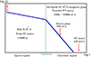 |
Fig. 7. Sketch of the georotator scenario evolution, showing the pulsar angular velocity evolution with time with the ejector and the georotator (present) phases and a dashed green line marking the transition. |
4.3. Lack of SNR evidence
As has been shown, in the georotator regime, the total time elapsed since the NS was formed can be ≫τ ∼ 500 yr, the age from Yoneda et al. (2020). There is first the period in which the pulsar was still in the ejector regime, which as explained may have lasted for ∼104 yr depending on the initial period and magnetic field. Then, in the georotator regime, the system may have evolved for some time until reaching the present stage, with a current decaying time of several centuries. Nevertheless, regardless of the georotator decaying time, since the multipolar magnetic field can be strong even when the NS rotation slows down, the actual magnetic field dissipation phase can last much longer (e.g., τmag ∼ 104 yr). From all this, the SNR may have occurred long ago and become by now already inconspicuous and difficult to detect.
Another, less likely, possibility for the absence of observational evidence of a SNR associated with LS 5039 could be a very small ejecta mass (e.g., up to 0.1 M⊙) in the case of a white dwarf (WD) turning into a NS (see eg. Woosley & Baron 1992; Kuroda et al. 2025). Such a scenario is unlikely as the rate of such a kind of SN explosion, particularly in high-mass binaries, is very low. Such a scenario may have occurred if the WD progenitor had transferred most of its mass to the secondary star, nowadays an O6.5 V star (Casares et al. 2005), preventing its initial direct collapse into a NS. In this quite improbable scenario, the NS might be quite young but no SNR would be visible.
4.4. The nonthermal emitter
The proposed scenario is not very different from the standard colliding wind scenario (e.g., Tavani & Arons 1997), as the former still features a relativistic outflow leaving the magnetosphere, but its power source is expected to be more irregular. Unfortunately, the simulations presented do not allow us properly connect the processes close to the NS with those on larger scales, and further work is required to properly characterize the development of an enhanced pulsar wind, and how it propagates and terminates, all of this in the context of the evolution of the whole interaction structure. It is known that the acceleration of electrons up to the required energies in LS 5039 is difficult (Khangulyan et al. 2008; Bosch-Ramon & Khangulyan 2025), and only an adequate characterization of that region can assess its ability to produce the particles with the required energies. Further downstream, the differences between the two scenarios are qualitatively smaller, although the more perturbed nature of the shocked flows due to magnetospheric flaring may suggest that particle acceleration on the scales of the spiral formation is stronger in that case. We emphasize that highly relativistic flows can still form outside the magnetosphere when strong flares occur, which can be a basic ingredient (as in the model proposed by Derishev & Aharonian 2012; Bosch-Ramon & Khangulyan 2025) for the production of ultra-high-energy photons such as those observed in LS 5039 (Alfaro et al. 2025). The overall nonthermal emitter is, however, likely to spread over a much larger region (e.g., Khangulyan et al. 2008; Bosch-Ramon et al. 2012). We finish by noting that the timescales inherent to the scenario explored here are diverse, from the light-crossing timescale of the magnetosphere (seconds) and the stellar wind crossing time of the interaction region (minutes to hours), to the orbital period (days).
We chose the normalization parameters to satisfy the following equation  with an accuracy better than 1%.
In reality, the interaction would be unlikely to correspond to two colliding supersonic winds, as it does here, but the simulation was set with such a configuration to simplify the numerical setup.
In a steady two-wind interaction (ejector) regime, this distance is roughly similar but somewhat larger than the pulsar wind termination shock radius.
We note that this estimate is not very robust and needs verification by multidimensional magnetohydrodynamical modeling.
Acknowledgments
The authors want to thank the referee for a useful report that helped to improve the clarity of the manuscript. VB-R acknowledges financial support from the Spanish Ministry of Science and Innovation under grant PID2022-136828NB-C41/AEI/10.13039/501100011033/ERDF/EU and through the María de Maeztu award to the ICCUB (CEX2024-001451-M), and from the Generalitat de Catalunya through grant 2021SGR00679. VB-R is Correspondent Researcher of CONICET, Argentina, at the IAR. Part of this work was supported by the Russian Science Foundation grant 23-22-00385 (sections 2 and 4) and BASIS foundation grant #24-1-2-25-1 (sections 1 and 3). The calculations were performed on CFCA XC50 cluster of the National Astronomical Observatory of Japan (NAOJ) and RIKEN HOKUSAI Bigwaterfall.
References
- Alfaro, R., Araya, M., Arteaga-Velázquez, J. C., et al. 2025, ApJ, 987, L42 [Google Scholar]
- Barkov, M. V., & Popov, S. B. 2022, MNRAS, 515, 4217 [Google Scholar]
- Barkov, M. V., Sharma, P., Gourgouliatos, K. N., & Lyutikov, M. 2022, ApJ, 934, 140 [Google Scholar]
- Barkov, M., Kalinin, E., & Lyutikov, M. 2024, PASA, 41 [Google Scholar]
- Barrère, P., Guilet, J., Raynaud, R., & Reboul-Salze, A. 2025, A&A, 695, A183 [NASA ADS] [CrossRef] [EDP Sciences] [Google Scholar]
- Beloborodov, A. M. 2020, ApJ, 896, 142 [NASA ADS] [CrossRef] [Google Scholar]
- Beskin, V. S. 2010, Phys. Usp., 53, 1199 [NASA ADS] [CrossRef] [Google Scholar]
- Bogovalov, S. V. 1999, A&A, 349, 1017 [Google Scholar]
- Bogovalov, S. V., Khangulyan, D., Koldoba, A., Ustyugova, G. V., & Aharonian, F. 2019, MNRAS, 490, 3601 [NASA ADS] [CrossRef] [Google Scholar]
- Bosch-Ramon, V., Barkov, M. V., Khangulyan, D., & Perucho, M. 2012, A&A, 544, A59 [NASA ADS] [CrossRef] [EDP Sciences] [Google Scholar]
- Bosch-Ramon, V., Barkov, M. V., & Perucho, M. 2015, A&A, 577, A89 [NASA ADS] [CrossRef] [EDP Sciences] [Google Scholar]
- Bosch-Ramon, V., & Khangulyan, D. 2025, A&A, 700, A162 [NASA ADS] [CrossRef] [EDP Sciences] [Google Scholar]
- Bozzo, E., Falanga, M., & Stella, L. 2008, ApJ, 683, 1031 [Google Scholar]
- Casares, J., Ribó, M., Ribas, I., et al. 2005, MNRAS, 364, 899 [Google Scholar]
- Collmar, W., & Zhang, S. 2014, A&A, 565, A38 [NASA ADS] [CrossRef] [EDP Sciences] [Google Scholar]
- Derishev, E. V., & Aharonian, F. A. 2012, in High Energy Gamma-Ray Astronomy: 5th International Meeting on High Energy Gamma-Ray Astronomy, eds. F. A. Aharonian, W. Hofmann, & F. M. Rieger (AIP), AIP Conf. Ser., 1505, 402 [Google Scholar]
- Igoshev, A., Barrère, P., Raynaud, R., et al. 2025, Nat. Astron., 9, 541 [Google Scholar]
- Illarionov, A. F., & Syunyayev, R. A. 1975, Why are there so few X-ray stars? [Google Scholar]
- Kargaltsev, O., Hare, J., Volkov, I., & Lange, A. 2023, ApJ, 958, 79 [NASA ADS] [CrossRef] [Google Scholar]
- Khangulyan, D., Aharonian, F., & Bosch-Ramon, V. 2008, MNRAS, 383, 467 [Google Scholar]
- Khangulyan, D., Barkov, M. V., & Popov, S. B. 2022, ApJ, 927, 2 [NASA ADS] [CrossRef] [Google Scholar]
- Kuroda, T., Kawaguchi, K., & Shibata, M. 2025, MNRAS, 541, 1649 [Google Scholar]
- Landau, L. D., & Lifshitz, E. M. 1980, The Classical Theory of Fields, 4th edn. (Butterworth-Heinemann) [Google Scholar]
- Li, S. 2005, J. Comput. Phys., 203, 344 [NASA ADS] [CrossRef] [Google Scholar]
- Lipunov, V. M. 1992, Astrophysics of Neutron Stars (Springer-Verlag Berlin Heidelberg New York) [Google Scholar]
- Lorimer, D. R., Bailes, M., McLaughlin, M. A., Narkevic, D. J., & Crawford, F. 2007, Science, 318, 777 [Google Scholar]
- Lyutikov, M., Barkov, M., Route, M., et al. 2020a, arXiv e-prints [arXiv:2004.11474] [Google Scholar]
- Lyutikov, M., Barkov, M. V., & Giannios, D. 2020b, ApJ, 893, L39 [NASA ADS] [CrossRef] [Google Scholar]
- Makishima, K., Uchida, N., Yoneda, H., Enoto, T., & Takahashi, T. 2023, ApJ, 959, 79 [Google Scholar]
- Mignone, A., Bodo, G., Massaglia, S., et al. 2007, ApJS, 170, 228 [Google Scholar]
- Moldón, J., Ribó, M., Paredes, J. M., et al. 2012, A&A, 543, A26 [NASA ADS] [CrossRef] [EDP Sciences] [Google Scholar]
- Mösta, P., Ott, C. D., Radice, D., et al. 2015, Nature, 528, 376 [CrossRef] [Google Scholar]
- Porth, O., Komissarov, S. S., & Keppens, R. 2014, MNRAS, 438, 278 [Google Scholar]
- Raynaud, R., Guilet, J., Janka, H.-T., & Gastine, T. 2020, Sci. Adv., 6, 2732 [NASA ADS] [CrossRef] [Google Scholar]
- Sharma, P., Barkov, M. V., & Lyutikov, M. 2023, MNRAS, 524, 6024 [Google Scholar]
- Spitkovsky, A. 2006, ApJ, 648, L51 [Google Scholar]
- Tavani, M., & Arons, J. 1997, ApJ, 477, 439 [NASA ADS] [CrossRef] [Google Scholar]
- Thompson, C., & Duncan, R. C. 1993, ApJ, 408, 194 [NASA ADS] [CrossRef] [Google Scholar]
- Weng, S.-S., Qian, L., Wang, B.-J., et al. 2022, Nat. Astron., 6, 698 [NASA ADS] [CrossRef] [Google Scholar]
- Woosley, S. E., & Baron, E. 1992, ApJ, 391, 228 [Google Scholar]
- Yoneda, H., Makishima, K., Enoto, T., et al. 2020, Phys. Rev. Lett., 125 [Google Scholar]
All Tables
All Figures
|
Fig. 1. Example of the time profile of a flaring period; δρ is the density on top of the regular pulsar wind density during flaring periods, x = 2πtNfl/Torb the dimensionless time (see Sect. 2.1 for details), and Δ = 0.1 the width of the pulse. |
| In the text | |
|
Fig. 2. Colored density maps on the orbital plane, with colored arrows representing the modulus of the 3-velocity vector for the 2D models. The flaring period rates are Nf = 90 (top left, 2Dn90e10), 30 (top right, 2Dn30e10), and 10 (middle left, 2Dn10e10) flaring periods per orbit, keeping the total energy budget of the system constant. In the model 2Dn30e30, we increased the power of the flaring period by a factor of 3, while keeping Nf = 30 (middle right panel). The non-flaring cases are presented at the bottom left (nfeta0.05) and right (nfeta0.5). |
| In the text | |
|
Fig. 3. Colored density maps with colored arrows representing the modulus of the 3-velocity vector for the 3D model (3Dn30e10) for various cuts: XY (top; orbital plane), XZ (middle), and ZY (bottom). |
| In the text | |
|
Fig. 4. Colored density maps with colored arrows representing the modulus of the 3-velocity vector for the 3D model (3Dn30e10) for cuts on the orbital plane, at orbital phases ϕ = 0.5435 (top left), ϕ = 0.575 (top right), ϕ = 0.5812 (middle left), ϕ = 0.6033 (middle right), ϕ = 0.6467 (bottom left), and ϕ = 0.6576 (bottom right). |
| In the text | |
|
Fig. 5. Zoom-in of three snapshots of the cycle followed by the interaction structure: weak pulsar wind (left), enhanced pulsar wind (middle), and the end of energy injection (right). |
| In the text | |
|
Fig. 6. Colored density maps obtained from an axisymmetric simulation showing qualitatively the evolution of a flare, from top left to bottom right: 0 (weak wind), 48 (flare starts), 88 (flare continuation), 141 (end of flare), 166 (pulsar wind approaches magnetosphere), and 186 s (flare about to resume) from the beginning of the flare. The grid size is ≈0.65 a; the magnetosphere radius would be ≈0.02 a in this case. |
| In the text | |
|
Fig. 7. Sketch of the georotator scenario evolution, showing the pulsar angular velocity evolution with time with the ejector and the georotator (present) phases and a dashed green line marking the transition. |
| In the text | |
Current usage metrics show cumulative count of Article Views (full-text article views including HTML views, PDF and ePub downloads, according to the available data) and Abstracts Views on Vision4Press platform.
Data correspond to usage on the plateform after 2015. The current usage metrics is available 48-96 hours after online publication and is updated daily on week days.
Initial download of the metrics may take a while.