| Issue |
A&A
Volume 703, November 2025
|
|
|---|---|---|
| Article Number | A132 | |
| Number of page(s) | 17 | |
| Section | Atomic, molecular, and nuclear data | |
| DOI | https://doi.org/10.1051/0004-6361/202556083 | |
| Published online | 13 November 2025 | |
SPECTCOL: A VAMDC tool for molecular spectroscopy and collisional data
1
LUX, Observatoire de Paris, Université PSL, Sorbonne Université, CNRS,
92190
Meudon,
France
2
Sorbonne Université, CNRS, MONARIS, UMR8233,
75005
Paris,
France
3
Departamento de Física, Facultad de Ciencias, Universidad de Chile,
Las Palmeras 3425,
7800003
Ñuñoa,
Santiago,
Chile
4
IRAP, Université de Toulouse, CNRS, CNES, UPS,
Toulouse,
France
5
LTE, Observatoire de Paris, Université PSL, Sorbonne Université, Université de Lille, LNE, CNRS,
61 Avenue de l’Observatoire,
75014
Paris,
France
★ Corresponding authors: This email address is being protected from spambots. You need JavaScript enabled to view it.
; This email address is being protected from spambots. You need JavaScript enabled to view it.
Received:
24
June
2025
Accepted:
9
September
2025
Abstract
Context. Modeling of atomic and molecular processes in the interstellar medium, especially in the case of nonlocal thermodynamic equilibrium requires combining spectroscopic and collisional data. This combination provides a so-called matching file that is an input file for radiative transfer codes.
Aims. We present the main functionalities of the SPECTCOL software that was developed in the environment of VAMDC standards: retrieving and exporting information from the CDMS, JPL, or HITRAN spectroscopic databases and the BASECOL collisional database, combining spectroscopic data and collisional data, and exporting the matching result in various formats.
Methods. The SPECTCOL software is a Java client.
Results. All molecules in the BASECOL database were tested with the SPECTCOL software, and the resulting matching files are available in a repository.
Conclusions. The SPECTCOL software and associated tutorials are available on the VAMDC website.
Key words: standards / astrochemistry / molecular data / radiative transfer / virtual observatory tools
© The Authors 2025
 Open Access article, published by EDP Sciences, under the terms of the Creative Commons Attribution License (https://creativecommons.org/licenses/by/4.0), which permits unrestricted use, distribution, and reproduction in any medium, provided the original work is properly cited.
This article is published in open access under the Subscribe to Open model. This email address is being protected from spambots. You need JavaScript enabled to view it. to support open access publication.
1 Introduction
The interstellar medium (ISM) is mostly characterized by high vacuum conditions where densities are much lower than 106 cm−3. This means that collisions are infrequent and that the assumption of local thermodynamic equilibrium (LTE) is generally not valid. The excitation temperature for each transition cannot be approximated by the kinetic temperature and now depends on the kinetic temperature and volume density. The level populations of atoms and molecules are determined by the balance between radiative and collisional processes and not by the gas kinetic temperature alone. Under these conditions, inelastic collisional rate coefficients are essential because they quantify the efficiency of collisions with H, H2, He, and electrons in exciting and deexciting molecular energy levels. H2 and He are the most abundant partners in the cold and dense regions of the ISM (possibly shielded regions) compared to H, He, and electrons in warmer gas (possibly irradiated regions). In comets within 2.5 au from the Sun (Biver et al. 2024), water is the main gaseous molecule in their atmosphere and so is the dominant collider. In more distant comets (Biver et al. 2024), however, CO and/or CO2 outgassing prevails, which makes these molecules the main colliders.
The collisional rate coefficients provide the critical input for non-LTE radiative transfer calculations, which allow us to accurately model the observed line intensities and derive key physical parameters of interstellar clouds and cometary atmosphere, such as density, kinetic temperature, and chemical composition. A striking manifestation of nonlocal thermodynamic equilibrium (non-LTE) excitation is the maser effect, where population inversions that are driven by a delicate interplay between radiative pumping and selective collisional processes produce coherent amplified microwave emission. CH3OH and OH masers have often been observed to trace shocked gas in star-forming regions such as outflows, but they also trace compact HII regions, supernova remnants, envelopes of evolved stars, and cloudcloud collision shocks in the Galactic center (e.g., Nesterenok 2022; Cragg et al. 2005). Without reliable collisional rate coefficients alongside spectroscopic data, interpretations of molecular spectra would remain highly uncertain, which would severely limit our ability to probe the physical and chemical state of the ISM or other media in non-LTE. Experimentally, collisional rate coefficients are difficult to measure and only cover a restricted range of temperatures and energy levels. Therefore, collisional rate coefficients have been widely and intensively computed for many molecules with various colliders and for wide ranges of temperatures and energy levels. These rate coefficients are compiled in databases such as BASECOL (a database for collisional data) (Dubernet et al. 2013; Ba et al. 2020; Dubernet et al. 2024), which can be used by astronomers for their non-LTE computations. The spectroscopic parameters are also necessary for the line identification and non-LTE modeling and are accessible through various databases such as CDMS (Cologne Database for Molecular Spectroscopy) (Endres et al. 2016), JPL (Jet Propulsion Laboratory) (Pearson et al. 2010), LSD (Lille Spectroscopic Database)1, the high-resolution transmission molecular absorption database (HITRAN) (Gordon et al. 2022), and the ExoMol (Tennyson et al. 2024) database for exoplanet studies (Bowesman et al. 2025) and other hot atmospheres, which are particularly useful with the recent advent of the James Webb Space Telescope. The basic ExoMol molecular database is very large, while its subset ExoMo1HR (Zhang et al. 2025), designed for spectral analysis, only provides transitions that are known to be highly accurate. It currently contains about 40% of the species in ExoMol. Because ExoMol is so very large, it has not been implemented in VAMDC (Virtual Atomic and Molecular Data Center2) (Dubernet et al. 2010; Dubernet et al. 2016; Albert et al. 2020), but a link to ExoMolHR would benefit the astronomy community, as would a link to the Lille Spectroscopic Database.
SPECTCOL is a specialized software tool designed to facilitate the management, analysis, and visualization of molecular spectroscopic and collisional datasets. Developed as part of the VAMDC infrastructure, SPECTCOL aims to bridge the gap between high-quality spectroscopic data and collisional rate coefficients. It allows researchers to perform matching operations and derive useful outputs for their studies.
At its core, SPECTCOL enables the retrieval, comparison, and combination of data from multiple VAMDC-connected databases, such as CDMS, JPL, and BASECOL. By integrating these datasets, SPECTCOL provides users with the capability to analyze the interaction between different molecular species, model radiative and collisional processes, and explore their effects in various environments, such as astrophysical or laboratory conditions. In addition, through VAMDC, SPECTCOL can also access, visualize, and export information from the HITRAN database.
The software supports a variety of output formats, including CSV (comma-separated values), XSAMS (XML schema for atoms, molecules, and solids) (Albert et al. 2020), and RADEX format, ensuring seamless compatibility with other tools and databases. The latter format is particularly interesting because it is the input file for the RADEX code (van der Tak et al. 2007), which is widely used by the astronomical community. It is a one-dimensional non-LTE radiative transfer code that uses the escape probability formulation assuming an isothermal and homogeneous medium without large-scale velocity fields. It is comparable to the large velocity gradient method and provides a useful tool for rapidly analyzing a large set of observational data providing constraints on physical conditions, such as density and kinetic temperature. With SPECTCOL, users can generate their own combined collisional-spectroscopic files that are ready to be ingested by RADEX in its standalone version or in the CASSIS3 software; the CASSIS software recreates the observed spectra with the use of an LTE model (through the excitation temperature, column density, and line width) and of a non-LTE-model (through the kinetic temperature, density of the collider, column density, line width, and the use of the collisional-spectroscopic files). Additionally, SPECTCOL allows the export of data into International Virtual Observatory Alliance (IVOA) tools4, thereby acting as a bridge between the VAMDC and IVOA infrastructures. Through these capabilities, SPECTCOL enables scientists to conduct their research efficiently while maintaining compliance with VAMDC standards for data exchange and interoperability.
Since the release of its first version (Dubernet & Nenadovic 2011; Dubernet et al. 2012), the front- and back-end of the SPECTCOL tool have both been completely redesigned, and new scientific features were added. The latest version of SPECTCOL is available for download on the VAMDC SPECTCOL website5: packages for different architectures are provided.
This paper is organized as follows: Section 2 outlines the VAMDC infrastructure and standards relevant to the design and usage of SPECTCOL. Section 3 describes the types of data retrieved from the CDMS, JPL, HITRAN, and BASECOL databases. Section 4 introduces the components of the SPECT-COL interface and their functionalities. Section 5 explains how to use SPECTCOL for visualizing and exporting data. Section 6 covers the functionality for combining spectroscopic and collisional datasets. Section 7 discusses current limitations, usage restrictions, and the validation procedures for the software. The conclusion presents some future perspectives.
2 VAMDC standards and molecular quantum numbers
2.1 General infrastructure
The VAMDC infrastructure provides a wrapper that connects approximately 37 heterogeneous atomic and molecular databases (the exact number may vary because new databases may join the federation and other may be temporarily disconnected due to maintenance). Detailed information about the VAMDC infrastructure, its terminologies is available in the consortium publications (Dubernet et al. 2016; Albert et al. 2020), Zwölf & Moreau (2023) provided a comprehensive description of architecture and standards adopted by the VAMDC infrastructure, and the consortium website includes detailed documentation. We list the key components and tools of the infrastructure below.
The VAMDC portal6 (Moreau et al. 2018) can be used to benchmark SPECTCOL data. Databases such as CDMS, JPL, and HITRAN can be visualized or exported in formats such as VOTable or JSON. The current visualization tool for molecular spectroscopy does not display line-broadening parameters, but the exported files contain all the data provided by the databases.
The Species database7 (Zwölf & Moreau 2024) facilitates interoperability of species across VAMDC-connected databases. Searching for species is aided by an autocompletion feature based on the various descriptions of species in the databases. The Species database is updated weekly by harvesting data from the VAMDC-connected databases. When a new species is added to a database between two harvests, it does not appear in the Species database immediately. Conversely, when a species is removed from a database, it will remain visible in the Species database for 45 days before it is permanently removed. This service is particularly useful for locating species across the VAMDC ecosystem and retrieving information such as the InChI, InChIKey8, and the so-called molecular stoichiometric formula. This formula is represented as an ASCII string of atomic constituents followed by their total counts (e.g., CH2O2 for formic acid, t/c- HCOOH). For molecular ions, the formula ends with a plus or minus sign. Table B1 presents the InchiKey of the molecules from the BASECOL database.
The SPECTCOL graphical user interface allows the user to select the VAMDC federated-databases (called data-nodes) to be queried. These data-nodes answer the query by returning an XML document structured following the XSAMS schema. XSAMS9 provides a standardized framework for describing atomic and molecular physics in terms of physical processes that connect different quantum states of atoms and molecules. A brief description of XSAMS can be found in Dubernet et al. (2016), while Endres et al. (2016) provided more details about the implementation of VAMDC standards for CDMS.
2.2 Standards for molecular quantum numbers (QN)
States of molecules are identified by tuples of the most relevant quantum numbers, with different tuples specified in XSAMS for various classes of molecules. This approach is known as the case-by-case standard10, which is currently maintained by the AMD unit11 of the IAEA12, a member of the VAMDC consortium.
Currently, there are 14 so-called cases, each corresponding to a specific type of molecule: diatomic, linear triatomic, nonlinear triatomic, linear polyatomic, symmetric top, spherical top, and asymmetric molecules. These are further divided based on their electronic states, which are categorized as either closed-shell or open-shell. For diatomic open-shell molecules, two cases are possible: hunda (Hund’s a coupling) and hundb (Hund’s b coupling).
The VAMDC nodes producing molecular data-outputs use these descriptions for the identification of molecular states. The cases of BASECOL molecules are indicated in Table B1, and issues related to cases are mentioned in Section 6.2.6.
2.3 Visualisation of QN with SPECTCOL
SPECTCOL follows the case-by-case standard for the display of QNs, such as J and N. We emphasize that users should consult the case-by-case documentation to understand the meaning of quantum numbers.
Some QNs have attributes that provide additional information: For example, Fj has two attributes, nuclearSpinRef and j, which characterize the nuclear spin couplings; I has two attributes, nuclearSpinRef and id; r has a single attribute, name; and vi and li each have one attribute, mode. The three lines below show XSAMS examples for I, vi, and li,
<lpcs:I nuclearSpinRef="H N" id="IHN">2.0</lpcs:I>
<lpcs:vi mode=4>2</lpcs:vi>
<lpcs:li mode=4>0</lpcs:li>
which are displayed as IIHN (total nuclear spin corresponding to the coupling of the nuclear spins of H and N), v4 (vibrational QN for the fourth vibrational mode), and l4 (vibrational degeneracy for the fourth vibrational mode). Currently, SPECTCOL ignores the nuclearspinref attribute because there is no standardization of the content of this attribute. SPECTCOL therefore indicates that users should check the scientific meaning of the hyperfine coupling before performing a matching between spectroscopic and collisional data.
Among the list of QN, the identifier r is a named positive integer label identifying the state when no other good quantum numbers or symmetries are known. This identifier might take any names, such as index1, as shown in the example below,
<lpcs:r name="index1">2.0</lpcs:r>.
When the attributes j, id, name, or mode are absent from the original files, SPECTCOL automatically substitutes these missing attributes with the value null. The associated QN is then displayed in red within the selection panel where QNs are designated for matching. This color-coding serves to indicate that matching with these particular QNs is prohibited to ensure clarity in the process.
In addition, sym, rotsym, vibsym, rovibsym, and elecsym have an attribute, group, and sym has an additional attribute, name. For now the attributes have not been implemented by the databases, so SPECTCOL currently ignores these attributes.
3 Description of the spectroscopic and collisional data
3.1 Spectroscopic data from the CDMS and JPL databases
The CDMS and JPL databases have been extensively described in the literature (Müller et al. 2001; Müller et al. 2005; Endres et al. 2014; Pickett 1991; Pickett et al. 1998; Pearson et al. 2010). Both databases provide spectroscopic data for molecular species that are (or might be) observed in various astronomical sources, primarily through radio astronomy.
Their traditional spectroscopic datasets are organized into individual entries displayed in the portals of the CDMS13 and JPL14 databases. Each dataset is identified by a TAG, which combines the mass number of the species (mainly molecules), and one digit, which is 5 for CDMS and 0 for JPL, with an incremental number to distinguish between datasets sharing the same mass number.
Additionally, each dataset is associated with a name, which is a character string indicating the species names, other global characteristics of the dataset (e.g., vibrational states), and the dataset version. Each dataset is also accompanied by documentation that provides information about the species, a description of the method used to produce the dataset, and references to the original papers in which the data were first published.
The traditional spectroscopic tables in the CDMS and JPL databases include several columns, as described on the CDMS website15. These columns include the frequency of the line (typically in MHz, but sometimes in cm−1), the uncertainty of the line (also usually in MHz, but occasionally in cm−1), the base-10 logarithm of the integrated intensity at 300 K (in nm2Hz), the degree of freedom in the rotational partition function (0 for atoms, 2 for linear molecules, and 3 for nonlinear molecules), the lower-state energy (in cm−1), the upper-state degeneracy (gup), the molecule TAG (where a negative value indicates that both the line frequency and uncertainty are experimental values), the CDMS or JPL coding for the quantum numbers, and the quantum numbers for the upper and lower levels of the line.
Additionally, the documentation section provides access to datasets in which the hyperfine structure is fully or partially resolved, along with the appropriate partition function files. The columns in the hyperfine datasets follow the same description as above. It should be noted that the upper state degeneracy is given by gup = gl × gF, where gl is the spin-statistical weight, and gF = 2 F + 1 is the upper-state spin-rotational degeneracy. The common factors in gl are often divided out, and the partition functions are consistent with these adjustments.
The VAMDC implementation (Endres et al. 2016) for both databases can be accessed via their beta portal16 and through any tool that supports the VAMDC protocols. These include the VAMDC portal, where the best visualization is achieved using the Molecular Spectroscopy XSAMS to HTML processor, astrophysical software such as CASSIS, or the library pyVAMDC17. The SPECTCOL visualization of the spectroscopic data tables is described in further detail in Section 4.3.2.
3.2 Spectroscopic data from HITRAN
The HITRAN database compiles molecular spectroscopic parameters for atmospheric species and currently covers 55 species. The latest version was described by Gordon et al. (2022). Data can be downloaded from the HITRAN website18 as customized ASCII files, allowing users to gather, for instance, different molecules or isotopologues within a specified wavenumber range.
Each molecule is assigned an arbitrary number (e.g., 1 for water) and a secondary number corresponding to a specific isotopologue, ranked in decreasing order of abundance (1 is the most abundant isotopologue). The line-by-line files contain the molecule number and isotopologue number, the wavenumber of the transition in cm−1, the intensity of the transition in cm−1/(molecule cm−2) at 296 K, the Einstein coefficient in s−1, the air-broadened half-width at 296 K, the self-broadened half-width at 296 K, the energy of the lower state in cm−1 , the temperature-dependence exponent of the air-broadened halfwidth, the air pressure-induced line shift, two sets of global quantum numbers for the upper and lower states, two sets of local quantum numbers for the upper and lower states, a group of six uncertainty indices for six parameters, a group of reference indices for the same parameters, and the statistical weights of the upper and lower states.
3.3 Collisional data from BASECOL
The BASECOL database collects relevant information and data from producers regarding the inelastic excitation of rotational, vibrational, and ro-vibrational levels of molecules by atoms, molecules, and electrons. The technical description of the newly designed BASECOL database (Ba et al. 2020) outlines the VAMDC access to BASECOL and the BASECOL implementation of VAMDC standards.
The BASECOL data are organized into collisional datasets, as described by Ba et al. (2020). These datasets represent collisions between a target (molecule or atom) and a projectile, referred to as the collider (molecule, atom, or electron). The VAMDC output and the traditional BASECOL website are both simultaneously updated with the latest versions of the recommended collisional datasets.
The BASECOL website and SPECTCOL both access the same underlying BASECOL database: The following description of datasets is therefore the same, regardless of how data are retrieved. For each collisional dataset, SPECTCOL retrieves and displays the rate coefficient table along with the associated energy tables, which identify the energy levels involved in the collisional transitions. These energy tables include the labels of the energy levels (called Index), their energy values (in cm−1 ), and the quantum numbers (QN) associated with the energy levels. The BASECOL database (Dubernet et al. 2024) accommodates inelastic processes that involve transitions between the target energy levels and, in some cases, between the collider energy levels, such as for H2.
Three types of rate coefficient tables are available: state-tostate, effective, and thermalized rate coefficients. For state-tostate rate coefficients, the first two columns (I1 and F1) indicate the initial and final states of the target, while the next two columns (I2 and F2) indicate the initial and final states of the collider. For effective and thermalized rate coefficients, BASECOL and SPECTCOL include effective or thermalized in the title of the collisional dataset. An effective rate coefficient table has identical entries in Columns 3 and 4, representing the initial level of the collider. A thermalized rate coefficient table has both Column 3 and Column 4 set to 1, and these labels do not carry any physical meaning.
In all cases, the remaining columns provide the rate coefficients (in cm3 s−1) as a function of temperature (in K). Dubernet et al. (2024) provide detailed equations for effective and thermalized rate coefficients: An effective rate coefficient is calculated for a specific initial state of the collider and corresponds to a summation of the state-to-state rate coefficients over the final states of the collider. A thermalized rate coefficient is obtained by performing a Boltzmann average of the effective rate coefficients.
4 SPECTCOL graphical user interface (GUI) components
4.1 General description
The SPECTCOL interface has four sections (see Fig. A.1):
The Help button provides a link to the tutorials.
The section Import data from file allows the upload of XSAMS files from the user’s local system. These files must come from BASECOL, CDMS, JPL, HITRAN, or be combined CDMS or JPL, and BASECOL datasets created by SPECTCOL (see Section 6). When they are uploaded, the datasets appear in the section Retrieved Radiative data and/or in the section Retrieved Collisional data.
The section Search VAMDC databases, which allows the selection and search of the databases.
The section Retrieved Radiative data, which displays the retrieved spectroscopic datasets, and where the matching process is initiated (see Section 6).
The section Retrieved Collisional data, which displays the retrieved collisional datasets, and where new collisional datasets can be created by scaling the retrieved data; the scaling leads to a fifth section. The scaled rate coefficients datasets are available for the matching process similarly to those included in the section Retrieved Collisional data (see Section 6).
All other panels are pop-up panels generated dynamically when functionalities are activated. These panels can be closed without shutting down the SPECTCOL GUI.
 |
Fig. 1 Query form for Species search. |
4.2 Search VAMDC databases
The section Search VAMDC databases enables users to select the relevant databases and to perform the queries on the selected databases. The databases must be selected before the queries forms are used. Although all VAMDC-connected databases can be reached, only CDMS, JPL, HITRAN, and BASECOL are allowed for queries.
The tab Species search and its associated query form allows the user to retrieve species information from the selected databases. The tab Collision & Radiative search allows the user to retrieve spectroscopic and collisional datasets. It includes the forms Collision, Radiative, and Collision & Radiative described below.
4.2.1 Species
In the form Species search (Fig. 1), a molecular species search is performed with the fields Molecular species InChIKey or the Molecular stoichiometric formula. It is also possible to specify the NuclearSpinIsomer, which can take the values para, ortho, meta, A, or E.
To search for an atomic species, use the Atomic Symbol with the list provided at the end of the VAMDC-XSAMS reference guide19, and the Ion Charge entries, which can be negative or positive integers. The field Particle Name accepts values such as photon, electron, muon, positron, neutron, alpha, or cosmic.
The result of the query Species search is displayed in a popup panel (as shown in Fig. A.2) with the following information: The source of the dataset, which includes the name of the queried database and the query timestamp, a comment column (optional content), the structural formula (as provided by the databases), the stoichiometric formula, the nuclear spin isomer characterization (if the molecular dataset includes only one nuclear spin), and the InChIKey. For CDMS and JPL databases, the comment column is a string composed of the TAG, of the same name as on their traditional entries and of the version. When a species is present in the databases with multiple datasets, a single output is provided.
As shown in Fig. A.2, the form Species search is useful to find all the available isotopologues in the four allowed databases using the Molecular Stoechiometric formula and to identify their InchiKey when those are not available in Table B1. This form provides very fast information as it does not retrieve any numerical data.
4.2.2 Collision
This form is used to search data from the BASECOL two-body collisional database. The target search is limited to molecules, while the collider (projectile) search includes molecules, atoms, and electrons. The search fields for the species are explained in the previous paragraph 4.2.1. It is advised to use Inchikey and specific collider, as well as spin isomer symmetry if it is relevant, in order to restrain the size of the retrieved datasets.
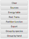 |
Fig. 2 Right panel of the section Retrieved Radiative data. |
4.2.3 Radiative
This form is used to search data from molecular spectroscopic databases. The search fields for the species are explained in the previous paragraph 4.2.1, and the other part of the query form allows to select ranges for spectroscopic quantities such as wavelength, upper- and lower-state energy of the transitions, and the Einstein A coefficient. The units for the spectroscopic quantities, apart from the Einstein A coefficient (in s−1), can also be selected for the search. The radiative search form is similar to the VAMDC portal search interface20.
4.2.4 Collision and Radiative
The option Collision & Radiative requests that molecular spectroscopic databases and BASECOL be selected, and performs both the Collision and the Radiative search. The retrieved datasets are displayed in the appropriate Retrieved sections. The main purpose of this option is to save time by reducing the number of queries, compared to querying first for collisional data and then for spectroscopic data. The drawback of this option is that retrieving data could take longer or fail if many or large datasets are involved.
4.3 Retrieved Radiative data section
4.3.1 General features
When the Radiative or Collision & Radiative search has been performed, the retrieved spectroscopic datasets are displayed in that section. The characteristics of the datasets follow the logic explained for the pop-up panel of the Species search (see section 4.2.1), with one additional parameter: the value of the VAMDC case (see section 2.2), as shown in Fig. A.3.
When a dataset is selected, the right panel (Fig. 2) of this section provides access to (1) the Sources functionality, which provides the references attached to the datasets, (2) the Energy table functionality, which displays the energy levels related to the upper and lower levels of the radiative transitions, (3) the Rad. Trans. functionality, which provides information on the radiative transitions, and (4) the Partition function functionality gives the partition function as a function of temperature as provided by the VAMDC output of the database. The tables of the above items (2), (3), and (4) are organized in columns that can be exported in CSV format, readable by commercial software, and can be sent via the SAMP protocol in the form of a VOTable to any IVOA tools such as TOPCAT (see Section 5). The functionalities Group by species and Group by hand correspond to the matching process between spectroscopic and collisional datasets, which is discussed in Section 6.
At this point, a distinction should be made between the molecular spectroscopic databases CDMS and JPL and the HITRAN database, which also includes line-broadening coefficients. In the current version of SPECTCOL, the right panel meets the scientific needs for displaying databases such as CDMS and JPL, but does not show line broadening. The function Export in XSAMS provides the complete dataset, however, including line broadening for HITRAN.
It must be emphasized that the VAMDC CDMS outputs of partition functions include all the available vibrational states, which is not always the case of the partition functions provided on the CDMS traditional websites. Their documentation21 indicates: “In general, only data for the ground vibrational state have been considered in the calculation of Q for a certain species. If excited vibrational states have been taken into account this will be mentioned in the documentation. Usually, individual contributions of the vibrational states are given in the documentation, too, or a link is given to a separate file containing the information”. In addition, the hyperfine partition functions are not transferred in VAMDC. Finally, we note that CDMS and JPL databases neglect the nuclear spin degeneracy both in the partition functions and in the degeneracy factors of the energy levels since these nuclear spin degeneracies factor out in the detailed balance equation. SPECTCOL does not display the HITRAN partition functions as those are not part of VAMDC output of HITRAN. The user is strongly advised to read the partition function documentation on the CDMS and JPL databases, and to recalculate their own partition functions. For the purpose of comparison with HITRAN partition functions, we note that HITRAN partition functions include the nuclear spin degeneracies.
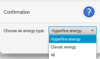 |
Fig. 3 Pop-up panel that gives the choice between the hyperfine, hyperfine unresolved data called classic energy, and the whole dataset. |
4.3.2 Energy tables and radiative transitions pop-up panels
When a dataset includes a mixture of hyperfine resolved and unresolved levels or transitions, the software prompts the user to select the type of data with which they wish to work (Fig. 3).
The Energy Table pop-up panels provide information on the energy levels involved in the radiative transitions. The tables are organized as follows: An index that identifies the level, its energy, the electronic state, the degeneracy, and the quantum numbers. The examples of Fig. A.4 and Fig. A.5 correspond to the choice of classic energy or hyperfine energy, with the title reflecting the type of spectroscopic data that were selected in Fig. 3. The radiative table (Fig. A.6) provides details on the radiative transitions, including the indexes of the upper and lower levels, which correspond to the indexes in the energy table, the frequency, the Einstein coefficient (in s−1 ), the uncertainty (when available), the upper degeneracy, and a column specific to the CDMS and JPL databases: the Log(Intensity), which is the base-10 logarithm of the integrated intensity at 300 K (see Section 3.1 and the CDMS website22).
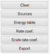 |
Fig. 4 Right panel of the section Retrieved Collisional data. |
4.4 Retrieved collisional data section
When the searches Collision or Collision and Radiative were performed on the BASECOL database, the retrieved collisional datasets are displayed in the section Retrieved Collisional data. For the target and the collider, the characteristics of the datasets follow the logic explained for the pop-up panel of the Species (see Section 4.2.1), with the additional VAMDC case parameter (see Section 2.2). It is important to note that the spin corresponds to the molecular nuclear spin characterization, so this column is empty for the atomic collider. The section Comment contains the title of the collisional dataset (identical to the one on the traditional website) and its version. The VAMDC implementation of BASECOL provides the latest version for the recommended datasets alone.
Similarly to the radiative section, the right panel of this section (Fig. 4) provides access to original data organized into Sources, Energy table, and Rate Coef., and it allows the user to download the datasets in XSAMS format via the Export functionality. The Energy table functionality allows the user to display the energy table linked to both the target and the collider. When the collider is an atom, the software can correctly interpret the atomic part of XSAMS for data coming from BASECOL alone.
In addition, the feature Scale rate coef. creates a new collisional dataset by scaling a selected rate coefficients dataset by a factor chosen by the user. This scaling feature can be used when a given rate coefficient table is used for another isotopologue or when rate coefficients for processes with H2 as a collider are obtained from rate coefficients with He as a collider.
The format of the rate coefficients displayed with the Rate Coef. or Scale rate coef. functionalities follow the description provided in Section 3.3. The energy and rate coefficients tables can both be saved in CSV format and exported via the SAMP protocol to an IVOA tool such as TOPCAT (see Section 5).
The Scale rate coef. functionality creates an additional section in the SPECTCOL GUI similar to the Collision part, displaying the newly created scaled collisional dataset, which can be combined with spectroscopic datasets. The right panel of this section has similar functionalities as the section Retrieved Collisional data.
4.5 Other characteristics
The Clear function requires selecting one or more datasets prior to activation, and it deletes the datasets from the display and memory.
Information panels: various hints are displayed in blue throughout the different windows that open from the main GUI. Warnings and error messages are provided. Additionally, some functionalities are activated and visible in pop-up panels when specific scientific situations (see Section 6.2) are encountered in the processed XSAMS files (e.g., when a spectroscopic dataset includes both hyperfine and hyperfine unresolved transitions, or when a collisional dataset includes transitions among the projectile’s levels).
5 Usage of SPECTCOL for visualization and for connection to IVOA tools
Currently, the spectroscopic data from CDMS, JPL, and HITRAN, and the collisional data from BASECOL can be visualized and exported. The spectroscopic and collisional energy tables, the table of spectroscopic transitions, and the table of collisional rate coefficients can be saved in CSV format or sent to IVOA tools (see below). The full spectroscopic dataset can be exported in XSAMS format and in the ASCII RADEX format. The collisional dataset can only be exported in XSAMS format.
The CSV and RADEX output files include references to the data and relevant units and explicitly include versioning information: 1) The version of each dataset used (collisional and spectroscopic) as indicated on the databases websites, 2) the version of the SPECTCOL software used to generate the output, 3) the exact date and time of the export. This ensures full traceability and reproducibility of results.
When an IVOA hub is active on the user’s machine (e.g., by launching an IVOA tool), SPECTCOL sends data files in VOTable format through the SAMP protocol23 to any IVOA tool that supports this protocol. For instance, the TOPCAT software24, as described on their website, is an interactive graphical viewer and editor for tabular data. Its purpose is to provide most of the tools that astronomers need for analyzing and manipulating source catalogs and other tables, although it can also be used for nonastronomical data. Therefore, users can access VAMDC molecular spectroscopic and collisional molecular data and process them in an environment suited for astronomers, allowing for transformation, comparison, and visualization.
SPECTCOL exports the energy tables, the Rad Trans table, and the collisional rate coefficients via SAMP. For the collisional rate coefficients, one option is to export all temperatures, which means that the table will plot the rate coefficients of a given transition as a function of temperature. Another option is one-by-one temperature, which allows users to plot rate coefficients for all transitions at a single temperature.
6 Matching of spectroscopic data and collisional data
6.1 Description of the matching process
To handle radiative transfer in non-LTE media, it is essential to combine spectroscopic and collisional data for the same transitions of the same observed (or target) molecule. This process, referred to as matching, is achieved by comparing the quantum numbers (QNs) of the energy levels involved in both the collisional and spectroscopic transitions. The QNs serve as the unique identifiers for the energy levels, making them key to this matching process. The user is advised to quickly review the spectroscopic and collisional energy tables before deciding which datasets to match and which QNs to select.
The option Group by hand (see Fig. 2) forces the matching of spectroscopic and collisional sets when a user wishes to combine collisional excitation rate coefficients (or scaled rate coefficients) of a molecule with the spectroscopic data of all its isotopologues. The option Group by species in the right panel restricts the matching to identical targets characterized by the same InChIKey.
The association between spectroscopic and collisional data works as follows. In step 1, only the energy levels that exist in both the collisional and the spectroscopic datasets are kept. This requires that the energy levels be described with the same case, and within that case, with the same quantum numbers. The selection is based on the quantum number values. In step 2, the unselected energy levels and associated energy transitions are removed from the original XSAMS files. In step 3, the energy levels of the collisional dataset are replaced by the spectroscopic energy levels, and the labeling of both the collisional and spectroscopic transitions is harmonized. The matching fails when no spectroscopic transitions are kept.
For hyperfine resolved transitions, the user must check whether the hyperfine couplings are similar in both the collisional and spectroscopic energy tables. A quick look at the quantum number nature and values provides an initial check. For a more thorough investigation, the user should consult the relevant information on the databases’ websites and possibly the original publications. It is important to note that each BASECOL collisional dataset contains only one type of case and one type of quantum number description. For example, hyperfine resolved levels are never mixed with pure rotational levels.
Finally, in the Energy table group pop-up panel, the user selects the relevant quantum numbers for the matching and performs the matching. The resulting page Matching result shows the energy table of the target molecule from the spectroscopic dataset, the rate coefficients table from the collisional dataset, the Einstein coefficients with the frequencies from the spectroscopic dataset, the energy table of the collider and finally the export/write section. The indexes of the target energy table identify the initial (I1) and final (F1) levels of the target in the rate coefficients table, as well as the upper and lower levels in the Einstein coefficients/frequencies section. The index of the collider energy table corresponds to the initial (I2) and final (F2) levels of the collider in the rate coefficients table.
The matched collisional and spectroscopic data can be saved in CSV, RADEX, and XSAMS formats. The matched XSAMS file can be re-imported into the SPECTCOL tool via the section Import data from file, where the option Collision & Radiative is selected. The display of the uploaded combined XSAMS file is split into the radiative and collisional retrieved displays, but the original BASECOL collisional energy table is replaced by the spectroscopic energy table. In the section Tutorial of the SPECTCOL webpage25 a video explaining the general usage of the software is provided.
6.2 Specific scientific situations
This section describes specific scientific situations that have been addressed by the SPECTCOL software. Any other specific situations not handled by the software must be managed externally by exporting the original collisional and spectroscopic data in CSV or XSAMS format.
6.2.1 Spectroscopic datasets partially filled with hyperfine levels
A single CDMS or JPL dataset might contain both hyperfine unresolved levels and hyperfine resolved levels. For example, see the CDMS HC3N dataset with TAG 51501-v1;HCCCN;v = 0. In contrast, a given BASECOL collisional dataset is always associated with a single ensemble of quantum number descriptions, such that hyperfine resolved levels are never mixed with hyperfine unresolved levels. For example, BASECOL contains rotational deexcitation datasets (Faure et al. 2016) for HC3N by p-H2 and o-H2 (38 levels; T=10-300 K), and datasets (Faure et al. 2016) for the deexcitation among hyperfine resolved rotational levels of HC3N by p-H2 and o-H2 (61 levels; T=10-100 K).
The first step involves selecting Group by species or Group by hand from the main panel, choosing the spectroscopic dataset TAG 51501-v1;HCCCN;v = 0 and either a hyperfine unresolved collisional dataset or a hyperfine collisional dataset, and then clicking Show selection. In order to select the correct spectroscopic energy levels and transitions, the software prompts the user to choose the energy type (either Hyperfine energy or Classic energy; the latter means hyperfine unresolved energy levels). The choice must align with the selected collisional dataset.
6.2.2 Collisional datasets with transitions between collider levels
We recall that BASECOL might include rate coefficients for collisional excitation involving both the target and the projectile species, which can be written as R(α → α′;β → β′)(T), where (α,β) and (α′,β′) represent the initial and final levels of the target (α) and projectile (β) (see section 2.4 in the last BASECOL paper (Dubernet et al. 2024) for more details). In the online display of the BASECOL database and in the CSV output files of SPECTCOL, α, β, α′, and β′ correspond to the notations I1, F1,I2, and F2, respectively. Most collisional datasets have I2 = F2 = 1, either because there is no transition within the projectile or because the levels of the projectile are considered thermalized (Dubernet et al. 2024). For collisional datasets where some transitions have I2 different from F2, there is always the option to match the rate coefficients for all collisional transitions by selecting All. In this case, only the CSV output is allowed because the RADEX format does not support transitions in the projectile. The other available choices correspond to I2 = F2 = X, which selects a subset of collisional transitions where I2 = F2 = X. This option allows RADEX outputs. For example, the rotational deexcitation among eleven rotational levels of CN− by p-H2 (Klos & Lique 2011) includes transitions between the projectile H2 ground state (level 1: j = 0) and first excited state (level 2: j = 2), and transitions corresponding to I2 = F2 = 1 or 2.
6.2.3 Addition of quantum numbers
Another situation arises when collisional datasets do not explicitly describe one or more quantum numbers, whereas the spectroscopic dataset includes those quantum numbers. This is often encountered with vibrational quantum numbers. SPECT-COL allows the user to add values to undefined quantum numbers. To do this, SPECTCOL indicates that missing quantum number values are selected and requests the inclusion of values. The value can be a single default value for all energy levels, or a series of values if the values must differ for individual energy levels.
For example, when matching a dataset (Balança et al. 2018) for the rotational deexcitation of SiO by p-H2 (21 rotational levels) with the CDMS dataset of TAG 44505-v2*;v = 0,10, the user is asked to select J and v as the matching quantum numbers and then to add the default value of 0 to v in the collisional data file. Another example is the usage of rotational rate coefficients calculated in the ground vibrational state for matching with rotational spectroscopy in another vibrational state: for example the collisional dataset of CS by p-H2 (Denis-Alpizar et al. 2018) with the rotational spectroscopic dataset with TAG 44501-v2*:CS;v = 0-4 can be used for v=0,1,2,4 (v = 0 and v = 1 matching datasets are indicated in Table B2). Spectroscopic datasets may sometimes also require additional implicit quantum numbers, and the procedure is similar.
6.2.4 Several energy levels with the same values of QN
The HITRAN datasets (Gordon et al. 2022) often contain several energy levels with the same values of quantum numbers but slightly different energy values. It is possible to visualize and export these spectroscopic datasets, but SPECTCOL will prevent any matching because it would lead to random results. The proper way to handle these datasets is to perform a pre-treatment to select one energy level from each set, and then proceed with the matching to collisional datasets.
The same issue arises if the chosen matching quantum numbers do not distinguish among energy levels, meaning that too few quantum numbers have been selected in the matching process. SPECTCOL detects this issue and requests the user to provide the correct selection of matching QNs. For example, when matching the collisional dataset (Lique 2010) for O2 by He with the CDMS spectroscopic dataset of TAG 32508-v2*;O2;X3Σ−; v = 0, the matching quantum numbers must be J and N. It is impossible for the user to perform a matching with N alone, for example.
6.2.5 Matching of ro-vibrational datasets
A collisional ro-vibrational dataset can cover several situations because it might or might not include rotational transitions. We list some examples below.
When a matching is made between a collisional rotational dataset in v = 0 and a ro-vibrational spectroscopic dataset without rotational transitions (e.g., the C3 by He (Ben Abdallah et al. 2008) collisional rotational dataset and the CDMS dataset TAG 36502-v1*:C3;v2 band), the matching does not work because there are no spectroscopic transitions among the selected matched energy levels.
When a matching is made between a collisional ro-vibrational dataset that does not include pure rotational transitions and a rotational spectroscopic dataset in several vibrational states (e.g., the CO by H (Song et al. 2015) collisional ro-vibrational dataset and the CDMS dataset TAG 28512-v1*;CO;v = 1,2,3), the matching is still possible, but cannot be used scientifically. The combined dataset includes rotational spectroscopic transitions with ro-vibrational rate coefficients between different vibrational states.
When a matching is made between a collisional ro-vibrational dataset that includes pure rotational transitions and a rotational spectroscopic dataset in a vibrational state (e.g., the 36ArH+ by He (García-Vázquez et al. 2019) collisional ro-vibrational dataset and the CDMS dataset TAG 37502-v1*:Ar-36-H+;v = 0), the matching provides a combined rotational datafile.
In addition, it might be possible to generate a complete ro-vibrational collisional-spectroscopic dataset in several steps, as shown in the following example:
When a matching is made between a collisional ro-vibrational set that includes rotational transitions and a ro-vibrational spectroscopic dataset with no rotational transitions (e.g., the CS by He (Lique & Spielfiedel 2007) collisional ro-vibrational dataset (114 levels with v=0,1,2 and 38 J in each vibrational state) and the CDMS dataset TAG 44510-v1*:CS v = 1-0; v = 2-1 bands), the matching might produce a file noted A. The rotational and ro-vibrational collisional transitions are both kept, but special attention should be paid to the scientific validity of having collisional rotational rate coefficients without corresponding spectroscopic rotational transitions.
As CDMS has a pure rotational spectroscopic set TAG 44501-v2*:CS v = 0,4, the user can perform a new matching with the CS by He (Lique & Spielfiedel 2007) collisional ro-vibrational dataset. Such matching, called B, will keep the full ro-vibrational collisional dataset and couple it to rotational spectroscopy in v = 0,1,2,3,4. As the labeling and sequence of energy levels is identical to the preceding matching called A, it is possible to extract the rotational spectroscopic transitions from B, and include them in the matched file A, to produce a file C. Nevertheless this matched file C has ro-vibrational collisional transitions between v = 2 and v = 0, and no corresponding spectroscopy.
Another matching can be performed between the same collisional ro-vibrational dataset (Lique & Spielfiedel 2007) and the CDMS dataset TAG 44511-v1*:CS v = 2-0. The resulting matched file D contain less energy levels and the labeling of energy levels and spectroscopic transitions are different from files A, B, C. A harmonization of the energy levels and transitions labeling of file D is necessary before copying the v = 2-0 spectroscopy in file C producing a final matched file E with fully matched ro-vibrational collisional and spectroscopic transitions among the 114 first ro-vibrational levels.
As a conclusion, special care must be taken to check the scientific validity of the combined datasets when ro-vibrational datasets are involved.
6.2.6 Other issues
SPECTCOL cannot handle matching with spectroscopic datasets where energy levels are not described with the same quantum numbers. These datasets can only be displayed and exported. This is the case for some HITRAN datasets (Gordon et al. 2022) that cannot be matched due to irregularities in the description of the energy levels, and this is currently the case for some JPL datasets. The issues have been reported to the database owners.
No matching is possible when the cases (see Section 2.2) are different between spectroscopic and collisional data. Modifying the quantum numbers and cases associated with the energy levels is beyond the scope of SPECTCOL; this issue should be addressed by the databases and data producers. For example, the Hund’s b case used for open-shell diatomic molecules in BASECOL is described with Hund’s a case in CDMS. Another example is the CH3OH molecule, which has different cases in CDMS and BASECOL.
7 Limitations and validation
A time-out may occur for very large datasets. In these cases, the user is encouraged to narrow the search metadata. When a timeout still occurs after the search is refined, the user is advised to contact the SPECTCOL maintainer.
7.1 Restrictions implemented in the software
We provide a summary of the current restrictions below.
The software splits the spectroscopic information into several files for CDMS and JPL; these files correspond to the original files that can be retrieved through the normal GUI of those databases. It is not currently possible to group spectroscopic datasets together in order to perform a matching with collisional data. For example, the software has a limitation when the spectroscopic databases provide ro-vibrational information in separate inputs.
Some spectroscopic inputs provide information for very high energies that might not be relevant for the scientific use cases. The user may want to apply an energy cut-off to perform the matching. Additionally, such a cut-off would remove unidentified high energy levels where the quantum number assignments do not strictly follow VAMDC standards. Currently, the software does not include an energy cut-off in the matching process, but it is still possible to reduce the spectroscopic dataset during the retrieval of spectroscopic data.
Badly formatted spectroscopic files with incomplete columns of QN values are not handled in the matching process. The user can use SPECTCOL to export the data in CSV or XSAMS format for further manipulation.
Original data files that include identical QN values for different energy levels are detected (e.g., HITRAN, some JPL files); these files cannot be matched. Since this situation is sometimes linked to human errors, SPECTCOL can be useful for detecting these issues.
During the matching process, if the user selects a set of QNs that does not distinguish some levels from others, the matching is not allowed.
SPECTCOL forbids matching when QNs are badly defined, such as when QNs are missing compulsory attributes (see Section 2.3).
SPECTCOL does not allow to add QN which have attributes (see Section 2.3 for explanations about attributes). This limitation could be lifted in the future if there is a strong scientific case.
7.2 Processes for validation of the software
This section presents the different steps we used to validate the SPECTCOL software. We tested the retrieved spectroscopic data, collisional data, and finally the matched data independently.
The spectroscopic validation of the SPECTCOL tool was made using the VAMDC portal, where we verified that the SPECTCOL outputs obtained via Rad. Trans. and Energy Table are the same as those obtained on the VAMDC portal. Since the SPECTCOL and VAMDC portal software were independently developed by different teams, this validation is meaningful. The comparison can be made either visually or automatically using the CSV outputs. This validation process does not ensure the scientific quality of VAMDC outputs from the spectroscopic databases, as their quality is the responsibility of the database providers. The SPECTCOL tool can sometimes be useful for identifying errors, however. Similarly, for collisional data, the energy table and the rate coefficients obtained with SPECTCOL are compared to the ASCII files from the BASECOL website. The spectroscopy of the matched data was again verified against the output from the VAMDC portal, while the collisional data of the matched data were verified against the BASECOL flat files, taking into account any changes in the labeling of the levels when these changes occurred.
The SPECTCOL tool was tested on the BASECOL2023 molecules (Dubernet et al. 2022) (see Appendix B) and on some molecules that were recently added. We recall that the BASECOL collisional datasets that are accessible through VAMDC correspond to the latest version of the recommended collisional datasets. Table B2 provides examples of matched datasets. The choice of datasets is made on selecting different use cases demonstrating the usage of functionalities of SPECT-COL, but does not constitute the reference set of RADEX from BASECOL. Some of the resulting ASCII files in RADEX and CSV formats are stored in a directory on ZENODO26 for the purpose of benchmarking the software.
8 Conclusion
The current version of the SPECTCOL tool can search the four VAMDC-connected databases CDMS, JPL, HITRAN and BASECOL, and match data from CDMS or JPL and BASECOL. When no matching is possible, SPECTCOL still provides useful information about energy levels and transitions through identifying quantum numbers, and the extraction in ASCII and CSV format of the data allows the user to further process the data with other tools. We recall that a matching fails when there is no spectroscopic transitions for the selected collisional transitions, and that SPECTCOL is not designed to solve scientific issues with the retrieved data (e.g., unresolved doublet energy levels of CH3CN in BASECOL cannot be matched with the doublet-resolved spectroscopic data in CDMS). A special warning must be set for the partition function: Although we facilitate access to the partition functions provided by CDMS and JPL, the VAMDC outputs must not be used without reading the molecule documentation of the CDMS and JPL websites. Finally, the retrieval of many and large files can take time.
While working with SPECTCOL, we noted that much spectroscopy is missing in order to provide matched datasets with the existing collisional datasets of BASECOL, and the reverse is true as well. Much work for many experimentalists and theoreticians therefore remains to provide data for the astrophysics scientific community.
As a future project, and only if the community supports the initiative, a Python version of the software might be provided via a notebook. An open-access Python version would allow users to develop their own solutions to overcome the limitations and restrictions embedded in the current SPECTCOL algorithm. Users are encouraged to report bugs when using the software. Additionally, the team would appreciate feedback on the use of the export to IVOA tools. The community should contact the SPECTCOL team27 for any reports or comments. The release version of SPECTCOL at the time of publication is version 2502_r1.
Acknowledgements
This work is part of the VAMDC consortium activities, of the National Observation Service F-VAMDC, and of Paris Astronomical Data Center (PADC) from the Observatory of Paris.
Appendix A Additional figures
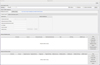 |
Fig. A.1 SPECTCOL GUI |
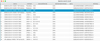 |
Fig. A.2 Example of results of the form Species search used with Stoechiometric formula = CHN on the four allowed databases. This retrieves spectroscopic and collision data corresponding to all isotopologues of HCN. |
 |
Fig. A.3 Example of results of the form Radiative used on CDMS database with InchiKey = LELOWRISYMNNSU-UHFFFAOYSA-N. This retrieves spectroscopic data related to the HCN molecule. |
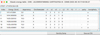 |
Fig. A.4 Energy table pop-up panel after selection of dataset 2 (TAG 27507) in Fig. A.3, and selection of Classic energy. |
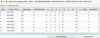 |
Fig. A.5 Energy table pop-up panel after selection of dataset 2 (TAG 27507) in Fig. A.3, and selection of Hyperfine energy. |
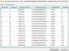 |
Fig. A.6 Radiative transitions table pop-up panel after selection of dataset 2 (TAG 27507) in Fig. A.3, and selection of Classic Einstein. |
Appendix B Tables
List of BASECOL molecules with InchiKeys and notes related to issues met with those molecules. Matched molecules are presented first.
Matched datasets between BASECOL collisional data and CDMS or JPL data. The selection does not reflect any quality assessments but aims to provide benchmark for all cases. Columns 1, 9, 10 provide the names of respectively the matched, collisional and spectroscopic files that can be found on ZENODO (https://doi.org/10.5281/zenodo.15691069). Column Levels indicates the number of matched levels.
References
- Albert, D., Antony, B., Ba, Y. A., et al. 2020, Atoms, 8 [Google Scholar]
- Amor, M. A., Hammami, K., & Wiesenfeld, L. 2021, MNRAS, 506, 957 [NASA ADS] [CrossRef] [Google Scholar]
- Ba, Y.-A., Dubernet, M.-L., Moreau, N., & Zwölf, C. M. 2020, Atoms, 8 [Google Scholar]
- Balança, C., Dayou, F., Faure, A., Wiesenfeld, L., & Feautrier, N. 2018, MNRAS, 479, 2692 [Google Scholar]
- Balança, C., Scribano, Y., Loreau, J., Lique, F., & Feautrier, N. 2020, MNRAS, 495, 2524 [Google Scholar]
- Balança, C., Quintas-Sánchez, E., Dawes, R., et al. 2021, MNRAS, 508, 1148 [CrossRef] [Google Scholar]
- Ben Abdallah, D., Hammami, K., Najar, F., et al. 2008, ApJ, 686, 379 [NASA ADS] [CrossRef] [Google Scholar]
- Biver, N., Russo, N. D., Opitom, C., Rubin, M., & Dotson, R. 2024, Chemistry of Comet Atmospheres (University of Arizona Press), 459-498 [Google Scholar]
- Bop, C. T. 2019, MNRAS, 487, 5685 [NASA ADS] [CrossRef] [Google Scholar]
- Bop, C., & Lique, F. 2025, A&A, 695, A132 [NASA ADS] [CrossRef] [EDP Sciences] [Google Scholar]
- Bop, C. T., Hammami, K., Niane, A., Faye, N. A. B., & Jaïdane, N. 2016, MNRAS, 465, 1137 [Google Scholar]
- Bop, C. T., Hammami, K., & Faye, N. A. B. 2017, MNRAS, 470, 2911 [NASA ADS] [CrossRef] [Google Scholar]
- Bop, C. T., Faye, N. A. B., & Hammami, K. 2018, MNRAS, 478, 4410 [NASA ADS] [CrossRef] [Google Scholar]
- Bop, C. T., Faye, N., & Hammami, K. 2019, Chem. Phys., 519, 21 [NASA ADS] [CrossRef] [Google Scholar]
- Bop, C., Kalugina, Y., & Lique, F. 2022a, J. Chem. Phys., 156, 204311 [NASA ADS] [CrossRef] [Google Scholar]
- Bop, C. T., Lique, F., Faure, A., Quintas-Sánchez, E., & Dawes, R. 2021, MNRAS, 501, 1911 [Google Scholar]
- Bop, C. T., Khadri, F., & Hammami, K. 2022b, MNRAS, 518, 3533 [CrossRef] [Google Scholar]
- Boursier, C., Mandal, B., Babikov, D., & Dubernet, M. L. 2020, MNRAS, 498, 5489 [NASA ADS] [CrossRef] [Google Scholar]
- Bowesman, C. A., Yurchenko, S. N., Al-Refaie, A., & Tennyson, J. 2025, TIRAMISU: Non-LTE radiative transfer for molecules in exoplanet atmospheres, https://arxiv.org/abs/2508.12873 [Google Scholar]
- Cabrera-González, L., Páez-Hernández, D., & Denis-Alpizar, O. 2020, MNRAS, 494, 129 [CrossRef] [Google Scholar]
- Cabrera-Gonzalez, L., Garcia-Vazquez, R., Paez-Hernandez, D., Stoecklin, T., & Denis-Alpizar, O. 2023, EPJD, 77, 107 [Google Scholar]
- Cernicharo, J., Spielfiedel, A., Balança, C., et al. 2011, A&A, 531, A103 [NASA ADS] [CrossRef] [EDP Sciences] [Google Scholar]
- Chandra, S., & Kegel, W. H. 2000, Astron. Astrophys. Sup., 142, 113 [Google Scholar]
- Chefai, A., Khadri, F., Alsubaie, N., Elabidi, H., & Hammami, K. 2024, MNRAS, 529, 4066 [Google Scholar]
- Cragg, D. M., Sobolev, A. M., & Godfrey, P. D. 2005, MNRAS, 360, 533 [Google Scholar]
- Dagdigian, P. J. 2020a, MNRAS, 494, 5239 [NASA ADS] [CrossRef] [Google Scholar]
- Dagdigian, P. J. 2020b, MNRAS, 498, 5361 [NASA ADS] [CrossRef] [Google Scholar]
- Dagdigian, P. J. 2021, MNRAS, 508, 118 [NASA ADS] [CrossRef] [Google Scholar]
- Daniel, F., Dubernet, M.-L., & Grosjean, A. 2011, A&A, 536, A76 [NASA ADS] [CrossRef] [EDP Sciences] [Google Scholar]
- Daniel, F., Faure, A., Wiesenfeld, L., et al. 2014, MNRAS, 444, 2544 [NASA ADS] [CrossRef] [Google Scholar]
- Daniel, F., Rist, C., Faure, A., et al. 2016, MNRAS, 457, 1535 [NASA ADS] [CrossRef] [Google Scholar]
- Demes, S., Lique, F., Faure, A., & van der Tak, F. F. S. 2022, MNRAS, 518, 3593 [NASA ADS] [CrossRef] [Google Scholar]
- Demes, S., Lique, F., Loreau, J., & Faure, A. 2023, MNRAS, 524, 2368 [NASA ADS] [CrossRef] [Google Scholar]
- Denis-Alpizar, O., Stoecklin, T., Guilloteau, S., & Dutrey, A. 2018, MNRAS, 478, 1811 [Google Scholar]
- Denis-Alpizar, O., Stoecklin, T., Dutrey, A., & Guilloteau, S. 2020, MNRAS, 497, 4276 [Google Scholar]
- Denis-Alpizar, O., Quintas-Sánchez, E., & Dawes, R. 2022, MNRAS, 512, 5546 [NASA ADS] [CrossRef] [Google Scholar]
- Denis-Alpizar, O., Guerra, C., & Zarate, X. 2023, A&A, 880, A113 [Google Scholar]
- Desrousseaux, B., Coppola, C. M., Kazandjian, M. V., & Lique, F. 2018, J. Phys. Chem. A, 122, 8390 [NASA ADS] [CrossRef] [Google Scholar]
- Desrousseaux, B., & Lique, F. 2020, J. Chem. Phys., 152, 074303 [NASA ADS] [CrossRef] [Google Scholar]
- Desrousseaux, B., Lique, F., Goicoechea, J. R., Quintas-Sánchez, E., & Dawes, R. 2021, A&A, 645, A8 [NASA ADS] [CrossRef] [EDP Sciences] [Google Scholar]
- Dubernet, M.-L., & Nenadovic, L. 2011, in Astrophysics Source Code Library [record ascl:1111.005], 11005 [Google Scholar]
- Dubernet, M.-L., & Quintas-Sánchez, E. 2019, Mol. Astrophys., 16, 100046 [NASA ADS] [CrossRef] [Google Scholar]
- Dubernet, M. L., Boudon, V., Culhane, J. L., et al. 2010, J. Quant. Spectrosc. Radiat. Transfer, 111, 2151 [NASA ADS] [CrossRef] [Google Scholar]
- Dubernet, M., Nenadovic, L., & Doronin, N. 2012, in Astronomical Society of the Pacific Conference Series, 461, Astronomical Data Analysis Software and Systems XXI, eds. P. Ballester, D. Egret, & N. P. F. Lorente, 335 [Google Scholar]
- Dubernet, M.-L., Alexander, M. H., Ba, Y. A., et al. 2013, Astron. Astrophys., 553, A50 [Google Scholar]
- Dubernet, M.-L., Antony, B., Ba, Y.-A., et al. 2016, J. Phys. B: At. Mol. Opt. Phys., 49, 074003 [NASA ADS] [CrossRef] [Google Scholar]
- Dubernet, M., Berriman, G., Barklem, P., et al. 2022, Proc. Int. Astron. Union, 18, 72 [Google Scholar]
- Dubernet, M. L., Boursier, C., Denis-Alpizar, O., et al. 2024, A&A, 683, A40 [NASA ADS] [CrossRef] [EDP Sciences] [Google Scholar]
- Endres, C., Schlemmer, S., Drouin, B., et al. 2014, in 69th International Symposium on Molecular Spectroscopy [Google Scholar]
- Endres, C. P., Schlemmer, S., Schilke, P., Stutzki, J., & Mueller, H. S. P. 2016, J. Mol. Spectrosc., 327, 95 [NASA ADS] [CrossRef] [Google Scholar]
- Faure, A., & Tennyson, J. 2003, MNRAS, 340, 468 [NASA ADS] [CrossRef] [Google Scholar]
- Faure, A., Gorfinkiel, J. D., & Tennyson, J. 2004, MNRAS, 347, 323 [NASA ADS] [CrossRef] [Google Scholar]
- Faure, A., Crimier, N., Ceccarelli, C., et al. 2007a, A&A, 472, 1029 [NASA ADS] [CrossRef] [EDP Sciences] [Google Scholar]
- Faure, A., Varambhia, H. N., Stoecklin, T., & Tennyson, J. 2007b, MNRAS, 382, 840 [Google Scholar]
- Faure, A., Wiesenfeld, L., Scribano, Y., & Ceccarelli, C. 2012, MNRAS, 420, 699 [NASA ADS] [CrossRef] [Google Scholar]
- Faure, A., Lique, F., & Wiesenfeld, L. 2016, MNRAS, 460, 2103 [NASA ADS] [CrossRef] [Google Scholar]
- Flower, D. R., & Lique, F. 2015, MNRAS, 446, 1750 [NASA ADS] [CrossRef] [Google Scholar]
- García-Vázquez, R. M., Márquez-Mijares, M., Rubayo-Soneira, J., & Denis-Alpizar, O. 2019, A&A, 631, A86 [NASA ADS] [CrossRef] [EDP Sciences] [Google Scholar]
- Gianturco, F. A., González-Sánchez, L., Mant, B. P., & Wester, R. 2019, J. Chem. Phys., 151, 144304 [NASA ADS] [CrossRef] [Google Scholar]
- Godard Palluet, A., & Lique, F. 2023, J. Chem. Phys., 158, 044303 [Google Scholar]
- Godard Palluet, A., & Lique, F. 2024, MNRAS, 527, 6702 [Google Scholar]
- Goicoechea, J. R., Lique, F., & Santa-Maria, M. G. 2022, A&A, 658, A28 [NASA ADS] [CrossRef] [EDP Sciences] [Google Scholar]
- Gong, Y., Henkel, C., Bop, C. T., et al. 2025, A&A, 696, A31 [NASA ADS] [CrossRef] [EDP Sciences] [Google Scholar]
- Gordon, I., Rothman, L., Hargreaves, R., et al. 2022, J. Quant. Spectrosc. Radiat. Transfer, 277, 107949 [NASA ADS] [CrossRef] [Google Scholar]
- Green, S. 1991, ApJS, 76, 979 [NASA ADS] [CrossRef] [Google Scholar]
- Guillon, G., & Stoecklin, T. 2012, MNRAS, 420, 579 [NASA ADS] [CrossRef] [Google Scholar]
- Hachani, L., Khadri, F., Jaïdane, N., Elabidi, H., & Hammami, K. 2024, MNRAS, 529, 4130 [Google Scholar]
- Hammami, K., Lique, F., Jaïdane, N., et al. 2007, A&A, 462, 789 [NASA ADS] [CrossRef] [EDP Sciences] [Google Scholar]
- Hammami, K., Nkem, C., Owono Owono, L. C., Jaidane, N., & Ben Lakhdar, Z. 2008, J. Chem. Phys., 129, 204305 [CrossRef] [Google Scholar]
- Hammami, K., Owono Owono, L. C., & Stäuber, P. 2009, A&A, 507, 1083 [NASA ADS] [CrossRef] [EDP Sciences] [Google Scholar]
- Hernández Vera, M., Lique, F., Dumouchel, F., et al. 2013, MNRAS, 432, 468 [CrossRef] [Google Scholar]
- Hernández Vera, M., Lique, F., Dumouchel, F., Hily-Blant, P., & Faure, A. 2017, MNRAS, 468, 1084 [Google Scholar]
- Kalugina, Y., & Lique, F. 2015, MNRAS, 446, L21 [NASA ADS] [CrossRef] [Google Scholar]
- Khadri, F., Chefai, A., & Hammami, K. 2020, MNRAS, 498, 5159 [NASA ADS] [CrossRef] [Google Scholar]
- Khadri, F., Hachani, L., Elabidi, H., & Hammami, K. 2022, MNRAS, 513, 6152 [Google Scholar]
- Klos, J., & Lique, F. 2008, MNRAS, 390, 239 [CrossRef] [Google Scholar]
- Klos, J., & Lique, F. 2011, MNRAS, 418, 271 [Google Scholar]
- Lanza, M., & Lique, F. 2012, MNRAS, 424, 1261 [NASA ADS] [CrossRef] [Google Scholar]
- Lique, F. 2010, J. Chem. Phys., 132, 044311 [NASA ADS] [CrossRef] [Google Scholar]
- Lique, F., & Spielfiedel, A. 2007, A&A, 462, 1179 [NASA ADS] [CrossRef] [EDP Sciences] [Google Scholar]
- Lique, F., Senent, M.-L., Spielfiedel, A., & Feautrier, N. 2007, J. Chem. Phys., 126, 164312 [NASA ADS] [CrossRef] [Google Scholar]
- Lique, F., Daniel, F., Pagani, L., & Feautrier, N. 2015, MNRAS, 446, 1245 [NASA ADS] [CrossRef] [Google Scholar]
- Mandal, B., & Babikov, D. 2023, A&A, 678, A51 [NASA ADS] [CrossRef] [EDP Sciences] [Google Scholar]
- Moreau, N., Zwolf, C.-M., Ba, Y.-A., et al. 2018, Galaxies, 6, 105 [Google Scholar]
- Müller, H. S. P., Thorwirth, S., Roth, D. A., & Winnewisser, G. 2001, A&A, 370, L49 [Google Scholar]
- Müller, H. S. P., Schlöder, F., Stutzki, J., & Winnewisser, G. 2005, J. of Mol. Struct., 742, 215 [Google Scholar]
- M’hamdi, M., Bop, C., Lique, F., Ben Houria, A., & Hammami, K. 2025, MNRAS, 536, 1791 [Google Scholar]
- Najar, F., Nouai, M., ElHanini, H., & Jaidane, N. 2017, MNRAS, 472, 2919 [NASA ADS] [CrossRef] [Google Scholar]
- Nesterenok, A. 2022, MNRAS, 509, 4555 [Google Scholar]
- Nkem, C., Hammami, K., Manga, A., et al. 2009, J. Mol. Struct.: THEOCHEM, 901, 220 [CrossRef] [Google Scholar]
- Pearson, J. C., Mueller, H. S. P., Pickett, H. M., Cohen, E. A., & Drouin, B. J. 2010, J. Quant. Spectrosc. Radiat. Transfer, 111, 1614 [Google Scholar]
- Pickett, H. M. 1991, J. Molec. Spect., 148, 371 [Google Scholar]
- Pickett, H. M., Poynter, R. L., Cohen, E. A., et al. 1998, J. Quant. Spectrosc. Radiat. Transfer, 60, 883 [Google Scholar]
- Pirlot Jankowiak, P., Lique, F., & Dagdigian, P. 2023a, MNRAS, 523, 3732 [NASA ADS] [CrossRef] [Google Scholar]
- Pirlot Jankowiak, P., Lique, F., & Dagdigian, P. J. 2023b, MNRAS, 526, 885 [NASA ADS] [CrossRef] [Google Scholar]
- Pirlot Jankowiak, P., Lique, F., & Goicoechea, J. R. 2024, A&A, 683, A115 [NASA ADS] [CrossRef] [EDP Sciences] [Google Scholar]
- Sahnoun, E., Nkem, C., Naindouba, A., et al. 2018, Astrophys. Space Sci., 363, 195 [NASA ADS] [CrossRef] [Google Scholar]
- Sahnoun, E., Ben Khalifa, M., Khadri, F., & Hammami, K. 2020, Astrophys. Space Sci., 365, 1 [CrossRef] [Google Scholar]
- Song, L., Balakrishnan, N., Walker, K. M., et al. 2015, ApJ, 813, 96 [NASA ADS] [CrossRef] [Google Scholar]
- Tennyson, J., Yurchenko, S. N., Zhang, J., et al. 2024, J. Quant. Spectrosc. Radiat. Transfer, 326, 109083 [Google Scholar]
- Terzi, N., Khadri, F., & Hammami, K. 2024, MNRAS, 532, 2418 [Google Scholar]
- Tonolo, F., Lique, F., Melosso, M., Puzzarini, C., & Bizzocchi, L. 2022, MNRAS, 516, 2653 [NASA ADS] [CrossRef] [Google Scholar]
- Urzúa-Leiva, R., & Denis-Alpizar, O. 2020, ACS Earth Space Chem., 4, 2384 [CrossRef] [Google Scholar]
- van der Tak, F. F. S., Black, J. H., Schöier, F. L., Jansen, D. J., & van Dishoeck, E. F. 2007, A&A, 468, 627 [NASA ADS] [CrossRef] [EDP Sciences] [Google Scholar]
- Walker, K. M., Song, L., Yang, B. H., et al. 2015, ApJ, 811, 27 [NASA ADS] [CrossRef] [Google Scholar]
- Walker, K. M., Lique, F., Dumouchel, F., & Dawes, R. 2017, MNRAS, 466, 831 [Google Scholar]
- Zhang, J., Hill, C., Tennyson, J., & Yurchenko, S. N. 2025, ApJS, 276, 67 [Google Scholar]
- Zwölf, C. M. & Moreau, N. 2023, Eur. Phys. J. D, 77, 70 [Google Scholar]
- Zwölf, C. M., & Moreau, N. 2024, Eur. Phys. J. D, 78 [Google Scholar]
- Zoltowski, M., Lique, F., Karska, A., & Zuchowski, P. S. 2021, MNRAS, 502, 5356 [CrossRef] [Google Scholar]
The InChIKey is an IUPAC product: https://iupac.org/who-we-are/divisions/division-details/inchi/ (International Union of Pure and Applied Chemistry). They can be found at: https://pubchem.ncbi.nlm.nih.gov/
All Tables
List of BASECOL molecules with InchiKeys and notes related to issues met with those molecules. Matched molecules are presented first.
Matched datasets between BASECOL collisional data and CDMS or JPL data. The selection does not reflect any quality assessments but aims to provide benchmark for all cases. Columns 1, 9, 10 provide the names of respectively the matched, collisional and spectroscopic files that can be found on ZENODO (https://doi.org/10.5281/zenodo.15691069). Column Levels indicates the number of matched levels.
All Figures
|
Fig. 1 Query form for Species search. |
| In the text | |
|
Fig. 2 Right panel of the section Retrieved Radiative data. |
| In the text | |
|
Fig. 3 Pop-up panel that gives the choice between the hyperfine, hyperfine unresolved data called classic energy, and the whole dataset. |
| In the text | |
|
Fig. 4 Right panel of the section Retrieved Collisional data. |
| In the text | |
|
Fig. A.1 SPECTCOL GUI |
| In the text | |
|
Fig. A.2 Example of results of the form Species search used with Stoechiometric formula = CHN on the four allowed databases. This retrieves spectroscopic and collision data corresponding to all isotopologues of HCN. |
| In the text | |
|
Fig. A.3 Example of results of the form Radiative used on CDMS database with InchiKey = LELOWRISYMNNSU-UHFFFAOYSA-N. This retrieves spectroscopic data related to the HCN molecule. |
| In the text | |
|
Fig. A.4 Energy table pop-up panel after selection of dataset 2 (TAG 27507) in Fig. A.3, and selection of Classic energy. |
| In the text | |
|
Fig. A.5 Energy table pop-up panel after selection of dataset 2 (TAG 27507) in Fig. A.3, and selection of Hyperfine energy. |
| In the text | |
|
Fig. A.6 Radiative transitions table pop-up panel after selection of dataset 2 (TAG 27507) in Fig. A.3, and selection of Classic Einstein. |
| In the text | |
Current usage metrics show cumulative count of Article Views (full-text article views including HTML views, PDF and ePub downloads, according to the available data) and Abstracts Views on Vision4Press platform.
Data correspond to usage on the plateform after 2015. The current usage metrics is available 48-96 hours after online publication and is updated daily on week days.
Initial download of the metrics may take a while.