| Issue |
A&A
Volume 703, November 2025
|
|
|---|---|---|
| Article Number | A180 | |
| Number of page(s) | 14 | |
| Section | Planets, planetary systems, and small bodies | |
| DOI | https://doi.org/10.1051/0004-6361/202556240 | |
| Published online | 13 November 2025 | |
Dust collisions in protoplanetary disks: From monodisperse to bidisperse grain aggregates
1
Instituto Interdisciplinario de Ciencias Básicas ICB, CONICET-FCEN UNCuyo,
Padre Contreras 1300,
5500
Mendoza, Mendoza,
Argentina
2
Instituto Argentino de Radioastronomía IAR,
CONICET-CICPBA-UNLP, CC No. 5, 1894 Villa Elisa,
Buenos Aires,
Argentina
3
Facultad de Ciencias Exactas y Naturales FCEN Sede Malargüe, UNCuyo, Campus Educativo Municipal II,
Rosario Vera Peñaloza esq. Fray L. Beltrán, 5613 Malargüe,
Mendoza,
Argentina
4
CONICET and Facultad de Ingenería, Universidad de Mendoza,
Paseo Dr. Emilio Descotte 750,
5500 Mendoza,
Mendoza,
Argentina
5
Centro de Nanotecnología Aplicada, Facultad de Ciencias, Universidad Mayor,
Camino la Pirámide 5750,
8580000 Huechuraba,
Santiago,
Chile
★ Corresponding author: This email address is being protected from spambots. You need JavaScript enabled to view it.
Received:
3
July
2025
Accepted:
12
September
2025
Abstract
Context. The coagulation of dust particles into pebbles is the first step of planet formation in protoplanetary disks. However, dust growth from micrometre-sized particles to pebble sizes has been linked to barriers that stand in the way of dust growth.
Aims. We investigate the roles of grain size, porosity, and impact velocity in collisions between equal-sized aggregates composed of monodisperse and bidisperse grains to determine the conditions that promote dust growth or fragmentation in protoplanetary disks.
Methods. We used discrete-element method (DEM) simulations to recreate collisions between granular aggregates with a given porosity, where the size of the constituent monomers can vary. Various in-house software tools were used for the sample generation and analysis of the results.
Results. Collisions between granular aggregates reveal that monomer size distribution strongly affects fragmentation outcomes. For monodisperse grain aggregates, smaller monomers favour adhesion and a sharp transition to fragmentation with steep fragment-size distributions, while larger monomers promote partial adhesion and shallower distributions. Bidisperse aggregates exhibit intermediate behaviour. Fragmentation velocity increases when monomers are smaller and porosity is higher. Coordination analysis shows that smaller grains allow more efficient reorganisation and compaction.
Conclusions. Monomer-size distribution plays a key role in determining the collisional evolution of aggregates. Together with porosity, these parameters strongly influence aggregate fragmentation and growth, with direct implications for dust evolution and pebble formation in protoplanetary disks. Our results support the inclusion of mixed-monomer aggregates in future collision models to better represent early planet formation processes.
Key words: methods: numerical / planets and satellites: formation / protoplanetary disks
© The Authors 2025
 Open Access article, published by EDP Sciences, under the terms of the Creative Commons Attribution License (https://creativecommons.org/licenses/by/4.0), which permits unrestricted use, distribution, and reproduction in any medium, provided the original work is properly cited.
This article is published in open access under the Subscribe to Open model. This email address is being protected from spambots. You need JavaScript enabled to view it. to support open access publication.
1 Introduction
Planet formation in protoplanetary disks is a complex process that is generally thought to begin with the coagulation of small dust particles to form aggregates. These aggregates collide with one another, with outcomes that include sticking, bouncing, abrasion, or fragmentation, depending on their properties, such as their size distribution, monomer material, and monomer size distribution, as well as the characteristics of the protoplanetary disk. When growth prevails over disruptive processes, aggregates form larger building blocks, known as pebbles, which range in size from millimetres to centimetres. This stage sets the foundation for the subsequent formation of planetesimals and planets.
Although pebbles play a critical role in state-of-the-art models of planetary formation, the formation of pebbles has been linked to barriers against dust growth, such as radial drift (Hyodo et al. 2021), bouncing barriers (Güttler et al. 2010; Zsom et al. 2010), and collisional fragmentation. However, such barriers are not well established, and discrepancies are sometimes found among experimental and numerical studies.
A key parameter that must be carefully considered is the collisional fragmentation threshold, which depends on several factors. Experimental studies have found fragmentation related to impact velocities above a few metres per second for colliding millimetre-sized dust aggregates of similar mass consisting of micron- or nanometre-sized silicate grains (Blum & Münch 1993; Güttler et al. 2010; Beitz et al. 2011; Blum 2018). This is relevant considering that relative collision velocities in protoplanetary disks can reach 60−100 m s−1 depending on the target-impactor size ratio and the turbulent gas velocity (Blum & Wurm 2008; Wurm & Teiser 2021). We ought to remember that the greater the difference in size between the target and the impactor, the greater the relative velocity between them due to the dependence of gaseous friction with the size of the aggregates in the protoplanetary disk (Weidenschilling 1997). In line with this correlation, experimental studies with high target-impactor size ratios report aggregate growth at high velocities. For instance, Teiser & Wurm (2009) performed experiments between centimetre- to decimetre-size SiO2 dust compact targets with only 67% porosity and submillimetre- to centimetresize SiO2 dust projectiles, finding growth for velocities up to 50 m s−1. Meisner et al. (2013) also observed growth for velocities up to 70 m s−1 for a target-impactor mass ratio of 1000 and the same material properties used by Teiser & Wurm (2009), confirming earlier findings that high-velocity collisions result in mass gain by the target for high target-impactor mass ratios.
Often, the aggregates used in experiments and simulations may have significantly different physical parameters, internal structures, and monomer properties, which can lead to discrepancies among results. Recent studies show that the threshold velocities separating fragmentation and coagulation regimes depend not only on the mass ratio between the colliding aggregates, but also on variables such as porosity and the properties of the monomers constituting the aggregates (Kimura et al. 2015; Ormel et al. 2007; Planes et al. 2020, 2021).
Porosity plays a critical role in dust aggregate behaviour in protoplanetary disks. The existence of porous particles in protoplanetary disks is well-supported by both theoretical models and experimental findings, which suggest that small dust particles coagulate to form fluffy agglomerates (Weidenschilling & Cuzzi 1993; Ormel et al. 2007; Krijt et al. 2015; Estrada et al. 2022). Experiments indicate that agglomerates ranging from millimetre to centimetre sizes (pebble-sized), which are unable to surpass the bouncing barrier in collisions, undergo compression, eventually reaching an equilibrium with porosity around 64% (Weidling et al. 2009; Zsom et al. 2010). Observationally, NIR scattered-light imaging has begun to provide insights into the porosity of small dust particles in protoplanetary disks. Notably, recent observations using the Very Large Telescope (VLT)/SPHERE have shown that all ten disks in their sample contain porous micron-sized dust particles with porosities ranging from 55% to 87% (Ginski et al. 2023). Moreover, observational studies using porous particles to fit multiwavelength continuum and millimetre-polarisation observations from the Atacama Large Millimeter/submillimeter Array (ALMA) and the Very Large Array (VLA) have inferred that the porosity of pebble-sized particles in the HL Tau disk ranges from 70% to 97% (Zhang et al. 2023). Molecular dynamics simulations have shown that the variation in porosity is a significant factor in collisional outcomes (Planes et al. 2020; Ormel et al. 2007; Gunkelmann et al. 2016), which has profound implications for the evolution of astrophysical systems composed of dust aggregates.
A grain is the smallest component of matter, being solid and homogeneous in composition. These monomers are the constituents that form the aggregates (Planes et al. 2020, 2021; Millán et al. 2025) and their size plays a crucial role in determining collisional outcomes (Kimura et al. 2015). Theoretical studies (Chokshi et al. 1993; Dominik & Tielens 1997) and experimental studies (Blum & Wurm 2008) suggest that the threshold velocity for sticking is approximately inversely proportional to the monomer size, implying that the inclusion of larger monomers generally decreases the sticking efficiency.
It is essential to consider whether the monomers in an aggregate are of a single size or a mixture of different sizes. While many studies in astrophysical scenarios have worked with aggregates composed of monodisperse monomers (Ringl et al. 2012; Wada et al. 2008, 2009; Planes et al. 2020, 2021), real aggregates often consist of monomers across a range of sizes (Güttler et al. 2019). Size polydispersity has received limited attention in astrophysical dust modelling. Umstätter et al. (2019) and Umstätter & Urbassek (2021a) simulated porous aggregates composed of one to five large grains, representing chondrules, with sizes ranging from 6 to 9 μ m, together with several hundred to several thousand small grains of 0.76 μ m. The grain size variability has been studied more extensively in other granular systems (see Millán et al. (2025) and references therein). Kimura et al. (2015) stated that it is unclear whether aggregates formed by particles of different sizes are mechanically weaker or stronger than aggregates made solely of monomers of the same size. These authors suggested that the net effect of monomer size variation should be clarified through future numerical and experimental studies.
Despite the limited investigation into the formation and evolution of aggregates composed of polydisperse grains, the aggregate size distribution in astrophysical settings is relatively well-constrained. Theoretical models of dust growth and fragmentation in protoplanetary disks incorporating processes such as turbulent stirring, radial drift, and coagulation have shown that dust follows a power-law size distribution with an exponent of −3. This is a natural outcome under a wide range of conditions (Birnstiel et al. 2012; Testi et al. 2014; Zhu & Yang 2021). This implies a steeper distribution towards smaller particles, suggesting that fragmentation and collisional processes are dominant. Observations from advanced facilities such as ALMA and VLA have uncovered intricate structures within protoplanetary disks, providing evidence for the presence of pebbles and smaller dust particles with size distributions that follow a powerlaw with an exponent close to −3 (Carrasco-González et al. 2019; Doi & Kataoka 2023; Sierra et al. 2021; Macías et al. 2019; Zhang et al. 2023). This is also confirmed by Spitzer infrared observations of the Zodiacal cloud in the Solar System (Trilling et al. 2020). These observations provide strong evidence for the ubiquity of this size distribution in protoplanetary disks. Also, cometary dust provides a unique opportunity to study primordial materials from the early solar nebula. Comets have been proposed to preserve pristine particles, offering a direct window into the properties of the early Solar System (Bentley et al. 2016). For example, studies by Lasue et al. (2009) and Kolokolova et al. (2003) demonstrate that cometary dust follows a similar power-law size distribution, with an exponent around −3, similar to that found in protoplanetary disks. These distributions are used to model the light scattering properties of cometary aggregates, providing valuable insight into the composition and size distribution of the particles. Furthermore, the analysis of dust collected from comets, such as those by the COSIMA experiment on Rosetta (Hilchenbach et al. 2016), reveals an average power-law exponent of −3.1 for the dust size distribution, with a range of sizes from 15 μ m to 225 μ m. This similarity in dust size distributions between protoplanetary disks and comets reinforces the idea that cometary dust can serve as a link to understanding the conditions in the early solar nebula, which is crucial to unravelling the mechanisms behind the formation of planetary bodies.
In this paper, we aim to advance our understanding of the role of porosity and monomer size in dust evolution and pebble formation by conducting numerical simulations that replicate interactions between micrometric silica dust. We study collisions between equal-sized porous aggregates in which all monomers have the same size within each aggregate, comparing cases with small monomers to those with large monomers. A key challenge of our study is incorporating more realistic porous aggregates, which better reflect actual astrophysical conditions. These aggregates include monomers of two different sizes and we also study collisions involving these more complex aggregates. All aggregates are generated using our recently published software (Millán et al. 2025). By varying the monomer size, their size distribution within the aggregates, and porosity, we aim to provide insights into the role these factors play in dust evolution and the formation of pebbles in protoplanetary disks.
In Section 2, we present a summary of our AGGENT aggregate generation software, the parameters of the simulations, and the analysis tools used. In Section 3, we present our results, along with relevant discussion. Finally, the conclusions and future work are outlined in Section 4.
Definitions, symbols, and abbreviations.
2 Materials and methods
In this section, we summarise the software used to construct the aggregates, AGGENT (Millán et al. 2025), along with the parameters selected for its configuration. Next, we describe the procedure for our simulations of collisions between pairs of equal-sized aggregates. The definitions, symbols, and abbreviations used in this work are listed in Table 1.
2.1 Aggregate building
Millán et al. (2025) has detailed how the software AGGENT constructs granular aggregates composed of monodisperse grains (meaning composed of identical grains) and composed of bidisperse grains (meaning composed of monomers of two different radii). While some previous studies have modelled the formation of polydisperse aggregates using dynamic simulations with frictionless particles (Estrada 2016; Oquendo-Patiño & Estrada 2020), we adopted a static approach for aggregate building that incorporates both adhesive and frictional forces to capture interparticle interactions more accurately. Details of the granular model are presented in Appendix A.
In this work, aggregates with various configurations were assembled using AGGENT. All aggregates were considered to be spherical, with a radius of Ragg=50 μ m. The material of the grains was assumed to be amorphous silica, whose parameters are detailed in Table 2.
Three different monomer size configurations were tested: Aggsg aggregates are composed of monodisperse grains with a radius of Rg=Rsg=0.5 μ m; Agglg aggregates are composed of monodisperse grains with a radius of Rg=Rlg=2.5 μ m; and Aggmix aggregates are composed of bidisperse grains, which are made of a mixture of grains with radii Rsg and Rlg. Table 3 presents the equilibrium distance, d0, (Eq. (A.4)) and the equilibrium overlap, δ0, (Eq. (A.5)) for the different grain sizes used in this study.
In the bidisperse case, the relationship μr between the number of grains Nsg, of a size Rsg, and the number of grains Nlg, of a size Rlg, is given by the condition that the radii Rsg and Rlg follow a power-law distribution, with an exponent of −3 (see Section 1). This results in the following number of grains of each size for aggregates with filling factor ϕ (defined as 1 – porosity)1 calculated as
 (1)
(1)
 (2)
(2)
Furthermore, two values of the filling factor ϕ were considered, ϕ=0.15 and ϕ=0.35 (Ginski et al. 2023; Zhang et al. 2023). Combining these values with the monomer size configurations results in six distinct aggregates. Table 4 details the number of grains of radius Rsg and Rlg, contained in each of these aggregates, according to their filling factor. A global view of each aggregate is shown in Figure 1.
Amorphous silica parameters used in this work.
Equilibrium distance, d0, and equilibrium overlap, δ0, between grains.
2.2 Simulations
The simulations performed in this work were executed in LAMMPS software (Thompson et al. 2022) using the JKR model (Johnson et al. 1971). Every simulation starts with two identical spherical aggregates separated by a short distance along the z-axis. There are six cases, each corresponding to a simulation with initial configurations of the colliding samples shown in Figure 1 and detailed in Table 4.
Each aggregate pair is given a set of velocities in opposite directions along the z-axis, each with a magnitude, v*, resulting in a relative velocity between them of v=2 v*. The time step used in all simulations is 5 × 10⁻¹¹ s (Ringl & Urbassek 2012). At the end of each simulation, two possible outcomes are considered for the results of the collisions (Wada et al. 2008):
fragmentation: the largest fragment has less than half of the total mass of the aggregates;
adhesion: a fragment is obtained that contains half or more of the total mass of the aggregates.
Some recent numerical studies on icy aggregates have reported an additional bouncing regime, whereby aggregates with radii larger than 300 μ m rebound rather than stick or fragment (Oshiro et al. 2025; Arakawa et al. 2023). This regime was observed for more compact and larger aggregates and different monomer properties and radii, which may explain why we did not observe such events in the lower filling-factor silica aggregates considered here.
Collision velocity is a fundamental factor in obtaining different results. The literature shows that fragment size decreases as collision velocity increases (Ringl et al. 2012; Wada et al. 2008, 2009). The fracture velocity, vfrac, is defined as the threshold above which the sample undergoes fragmentation following the collision. For each of the six simulation cases, a range of velocities, v, was tested to determine the velocity, vfrac, that separates the fragmentation and adhesion regimes. Another relevant aspect is obtaining the size distribution of the fragments resulting from the collisions; the methods used for this purpose are detailed in Appendix B.
The simulations were run until no significant changes were observed in the final structure, which means no differentiation in the number and size of the fragments. To report the numerical error, the aggregates were rotated and the simulations were repeated. The errors in the number of fragments obtained after the collision and in the fracture velocity were found to be less than 10% for the six simulation cases.
The execution times of the simulations varied considerably among the six simulation cases. The main determining factor was the total number of grains, Ng. Execution times ranged from 45 minutes for sample 3 (Ng=2542) to 72 hours for sample 2 (Ng=714 734).
Initial configurations of the aggregates.
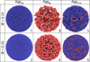 |
Fig. 1 Global view of each aggregate type with ϕ=0.15 and ϕ=0.35. Blue and pink grains correspond to Rg=0.5 μ m and Rg=2.5 μ m, respectively. Numbers refer to the cases listed in Table 4. |
3 Results and discussion
In this section, the results obtained from a series of simulations are presented, where the following parameters were varied: the radius Rg of the monomers composing the aggregates, the filling factor ϕ of the aggregates, and the collision velocity, v, which ranged from 1 to 50 m s−1. It is typically assumed that aggregates with radii of ∼50 μ m are expected to collide at ∼0.1−1 m s−1 depending on local disk conditions (Blum & Wurm 2008). However, Carballido et al. (2010) found, assuming that turbulence is generated by magnetorotational instability, that relative velocities in a protoplanetary disc may be as high as the sound speed for values of the viscosity parameter α of ∼10−2 and minimum mass solar nebulae conditions. Carballido et al. (2010) calculated relative velocities as functions of particle Stokes number St. The grey vertical band in their Figure 5 represents the approximate range of disruption velocities (0.1−10 m s−1) as found in Ormel et al. (2007); Dominik et al. (2007); Blum & Wurm (2008). However, Carballido et al. (2010) also shows in their Figure 5 that the peak of their distributions of relative velocities for different values of St are at relative speeds of the order of 10−100 m s−1, in line with our choosing of collision velocities as high as 50 m s−1. High collision velocities among aggregates are also useful for the study of dust collision in cometary comas (Planes et al. 2024), in planetary rings and debris disks, as well as asteroid rings (Beitz et al. 2016).
3.1 Collisional evolution for different aggregate types
We show three examples of the collisional evolution of aggregates of different types. We first analysed collisions between two aggregates composed of monodisperse grains and we later analysed the collision between two aggregates composed of bidisperse monomers.
In Figure 2a, we show the time evolution of a collision with velocity v between two Aggsg aggregates (Ragg=50 μ m and Rg= Rsg=0.5 μ m) with ϕ=0.35 (case 2 of Table 4) and in Figure 2b, we show the time evolution of a collision with velocity v between two Agglg aggregates (Ragg=50 μ m and Rg=Rlg=2.5 μ m) with ϕ=0.35 (case 4 of Table 4). The colour-coding indicates the magnitude of the velocity vi (in m s−1) of each i-monomer.
In Figure 2a, which corresponds to the case of small monodisperse monomers, we observe:
at t=0, each aggregate moves towards the centre of mass of the system with a velocity of 20 m s−1; thus, the relative collision velocity of the aggregates is v = 40 m s−1;
at t=2.5 μ s, the aggregates have merged into a single entity, with numerous collisions among monomers near the collision area, resulting in a velocity reduction due to intergranular dissipative processes. However, regions near the poles still retain their initial velocity. A belt of grains ejected at high velocity is observed around the equator;
at t=15 μ s, the sample is flattened into a disk shape. The velocity, vi, of the grains is minimal at the centre and increases radially towards the edges. A large number of grains and ejected fragments are observed;
at t=50 μ s, the simulation displays the final system of fragments. The largest fragment consists of 47279 grains, representing 6.6% of the total sample. This is a clear example of complete fragmentation, where none of the fragments make up half or more of the total system mass.
In Figure 2b, which corresponds to the case of large monodisperse monomers, we observe:
again, at t=0, the aggregates approach each other, each moving with a velocity of 3.5 m s−1, so the relative velocity, v= 7 m s−1, is lower compared to the case shown in Figure 2a.
at t=10 μ s, the aggregates encountered each other, forming an ellipsoidal body with minimum velocity vi at its centre. Once again, grains at the poles experienced the last changes in velocity due to their further distance from the collision zone. Compared to the case shown in Figure 2a, a more diffuse shockwave is observed;
at t=40 μ s, there is a drastic decrease in vi, with some grains and small fragments ejected;
at t=100 μ s, a large fragment is observed, resembling an almost flattened disk and containing nearly all of the grains in the sample (99.5%), with vi approaching zero. In this case, the collisional outcome is adhesion with minor erosion caused by ejected grains.
In all simulated cases, there is a notable decrease in the velocity, vi, of the grains in the system as the collision progresses. This is due to the frictional forces associated with the various degrees of freedom that the motion between interacting grains can exhibit (see Appendix A and Section 2.2). Previous studies have shown that these intergranular frictional forces dissipate the majority of the energy in granular systems (Planes et al. 2019).
The initial relative velocity, v, of the aggregates has only a vertical (z) component. After the collision, the samples undergo flattening. The grains belonging both to the resulting final aggregate and to ejected fragments have velocities vi primarily lying in the x−y plane. This is correlated with the linear momentum transfer previously analysed by Planes et al. (2020).
We should point out that for all cases analysed, erosion increases as the collision velocity v increases, reaching the so-called fragmentation velocity, vfrac, beyond which the sample is considered to belong to the ‘fragmentation’ outcome defined in Section 2.2. This issue is discussed in Sections 3.2 and 3.3.
Finally, we analysed a collision between two aggregates composed of bidisperse monomers. Figure 3 shows the time evolution of a collision with velocity v = 10 m s−1 between two aggregates type Aggmix(Ragg=50 μ m, Rsg=0.5 μ m., and Rlg= 2.5 μ m) with ϕ=0.35 (case 6 of Table 4). The colour-coding indicates the magnitude of the velocity vi (in m s−1) of each i monomer. We can observe from the temporal evolution of this collision the following characteristics.
initially, the simulation begins with two identical spherical aggregates separated by a short distance, each having an initial velocity magnitude of 5 m s−1.
at t=10 μ s, the aggregates have made contact and it is notable that there are similarities with the simulations previously presented in Figure 2. Compared to Figure 2a at 2.5 μ s, a similar effect is observed, with grains at the poles maintaining their velocity, while others at the equator are ejected. The difference now lies in the fact that a well-marked wave front cannot be distinguished, which is an effect that is analogous to that observed at t=10 μ s in Figure 2b. Thus, the samples composed of bidisperse grains analysed here lead to an intermediate case between those observed for samples composed of small and large monodisperse grains shown in Figure 2.
at t=60 μ s, we have the final state of the simulation. There is partial adhesion with a large percentage of the sample concentrated in a larger central fragment (91%) with ejection of some smaller fragments and grains. This is an intermediate case between the two scenarios presented in Figure 2, featuring a large final aggregate that contains more than 50% of the total mass, similar to the large fragment observed in the final state of Figure 2b. However, it also shows ejected material in the form of smaller fragments and monomers, resembling the small fragments ejected in the case shown in Figure 2a.
We can see from Figures 2 and 3 that the size distribution of the ejected fragments shows differences between the various cases discussed. Next, we study the dependence of the size of the final fragments on the collision velocity and examine how the monomer size that forms the aggregate influences these outcomes.
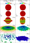 |
Fig. 2 Temporal evolution of a collision between aggregates composed of identical grains. (a) Simulation of case 2: Rg=Rsg=0.5 μ m with ϕ=0.35. (b) Simulation of case 4: Rg=Rlg=2.5 μ m with ϕ=0.35. The colour-coding indicates the magnitude of the velocity vi of each particle. |
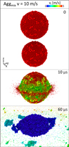 |
Fig. 3 Temporal evolution of a collision with v = 10 m s−1 between aggregates composed of bidisperse grains. Simulation of case 6: Rsg = 0.5 μ m and Rlg=2.5 μ m with ϕ=0.35. The colour-coding indicates the magnitude of the velocity vi of each particle. |
3.2 Fragment distribution
The final fragments, defined as those with fewer than 100 grains (n<100), are identified following the methodology described in Appendix B. F(n) represents the number of fragments composed of n monomer grains. The distribution of the final fragments, F(n), depends on the number of particles, n, in the fragment as follows:
 (3)
where k and s are constants and N=2 Ng is the total number of grains.
(3)
where k and s are constants and N=2 Ng is the total number of grains.
Figure 4 shows the distribution of fragments resulting from simulations with v = 10 m s−1 for all cases. For the six cases of Table 4, there is a predominance of isolated ejected monomers (n=1) with a subsequent drop in frequency as n increases. For the smaller fragments, the data points for each sample can be fitted by a straight line with a negative slope. However, this trend is lost for larger fragment sizes. Two fitted lines consistent with Eq. (3) were plotted: the blue dotted line corresponding to case 1 with a slope s=2.72 and the green dotted line corresponding to case 3 with slope s=1.74. Higher s values indicate a greater predominance of monomers and small ejected fragments.
Planes et al. (2021) carried out granular-mechanics simulations to study the influence of porosity and impact velocity in collisions of spherical granular aggregates with different mass ratios, but the same monomer size. They found that the number of monomers in the final fragment distribution followed a power-law, in accordance with Eq. (3) and with previous works referenced therein (Biswas et al. 2019; Kun et al. 2019; Kobayashi & Shibayama 2021; Akiba et al. 2023; Pueyo 2011; Ishii & Matsushita 1992). Their simulations were carried out using aggregates composed of monomers with Rg=0.76 μ m, similar to those of radius 0.5 μ m employed in this work. Planes et al. (2021) found an exponent of approximately s=2.8, independent of the collision velocity, the projectile-target mass ratio, and the porosity. The blue fit in Figure 4, corresponding to case 1, shows excellent agreement with Planes et al. (2021), and the exponent also matches the results for case 2, which has different porosity. Both cases, 1 and 2, are aggregates composed of grains of size 0.5 μ m, similar to the size used in Planes et al. (2021) with different filling factor values (0.12 ≤ ϕ ≤ 0.40). Therefore, for small monomers, our results are in agreement with that work, and we conclude that the distribution of fragments does not appear to show a dependence on the porosity of the samples.
However, the green adjustment performed for case 3 gives an exponent s=1.74, which also fits the results of case 4, very different from the exponent obtained for cases 1 and 2. Based on the values of s for cases 1 to 4 (monodisperse monomers), we observe that fragments originating from aggregates composed of smaller grains exhibit a greater number of monomers and dimers than those from aggregates composed of larger grains. We conclude that, at least at low velocities, the fragment distributions follow a power-law whose exponent appears to depend more on the grain size than on the porosity of the aggregates.
The mixed samples deviate slightly from the blue fit, showing higher s values. For case 5, the fit gives s=3.3 and for case 6, s=3.1. Although large grains (size Rlg) account for only 0.8% of the total, compared to 99.2% for small grains (size Rsg), they are highly relevant to the resulting distribution. It is worth noting that the exponent found for the collisions between aggregates Aggsg(s=2.72) provides a good fit for the fragments from collisions between aggregates Aggmix, when these fragments contain five or more particles. This indicates that the difference is primarily relevant in the frequencies of the smaller ejected fragments, mainly monomers and dimers.
In other studies, similar values of s have been reported for the fragment distribution of aggregates with fewer than 100 particles. For example, Paszun & Dominik (2009) examined collisions of both compact and fluffy aggregates with monomers of 1.2 μ m in diameter. They observed that the slopes of the fragment distributions ranged from approximately 0.3 to nearly 3 (see their Fig. 4). They proposed that, although the compactness and structure of the aggregates may be important, the main factor determining the collisional outcome is the kinetic energy of the impact.
In addition, Bandyopadhyay & Urbassek (2023) reported an s value between 1.5 and 2 for the fragment distribution resulting from collisions between granular aggregates with a monomer size of 0.76 μ m (comparable to Rsg) and a filling factor of ϕ= 0.24. However, the total number of particles in their aggregates was 20000, a value closer to the Ng in our cases 3 and 4 than to those in cases 1 and 2 (see Table 4). This suggests that, in addition to the monomer size, there may also be an influence from the ratio between the aggregate’s size and the grain’s size. Specifically, it may not just be the monomer size that influences the fragmentation, but rather how the size of the monomers relative to the size of the aggregate affects the available surface area for interaction, as adhesion primarily depends on surface area.
To analyse what happens at higher velocities where the ejecta is greater, we show in Figure 5 the distribution for minor fragments for simulations with velocity v=40 m s−1. Again, the curves described by Eq. (3) can be fitted to these distributions.
For the fit of case 1, a value s=2.66 was obtained (blue dashed line in Fig. 5). This value is very similar to the fit of the same case obtained with collision velocity v = 10 m s−1 shown in Figure 4. A similar exponent fits the data for case 2 as well. This indicates that, for aggregates composed of small grains, the exponent s appears to be independent not only of porosity but also of collision velocity, in agreement with the findings of Planes et al. (2021). The nearly velocity independence of the power-law exponent for our Aggsg aggregates aligns with the weak velocity dependence found by Arakawa et al. (2022) and Hasegawa et al. (2023) for icy aggregates, suggesting that this nearly velocity-independent behaviour may hold across different materials, although further studies are needed to test this. The fit for case 3 has a value s=1.97 (green dashed line in Fig. 5), which is slightly higher than the value obtained for the collision at v = 10 m s−1 (Figure 4). However, now with a collision velocity of 40 m s−1, the difference between the exponents (s=2.66 and s=1.97) is smaller. For case 4 (red full squares), the fit with s=1.97 holds if monomers and dimers are not considered. However, when the complete distribution, including monomers and dimers, is taken into account, the fit gives an exponent s= 1.5. Although a more in-depth analysis is required, it seems that porosity might become relevant in the case of aggregates formed by grains of 2.5 μ m.
Finally, we observed that at high collision velocities, where all samples undergo fragmentation, the fit for the mixed samples appears to be similar to that obtained for case 1 (blue dashed line). In other words, the exponent s=2.66 provides a reasonably good fit for cases 1, 2, 5, and 6. It is then understood that at higher v, the influence of the large grains within the aggregates Aggmix on the resulting fragment distribution decreases. The values for the exponent s of Eq. (3) obtained from the fitting for all cases are reported in Table 5.
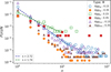 |
Fig. 4 Fragment distribution, F(n), for simulations with a collision velocity of v = 10 m s−1. |
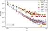 |
Fig. 5 Fragment distribution F(n) for simulations with collision velocity v = 40 m s−1. |
3.3 Fragmentation velocity
The simulations were conducted within the framework of the coagulation process, in which adhesion between grains leads to the formation of pebbles and larger bodies. Understanding how micrometric dust grains stick to each other is key to comprehending dust coagulation during the early stages of planetary formation in protoplanetary disks. The maximum collision velocity in a protoplanetary disk is important to determine the fate of the aggregates and is given by the difference between the Keplerian speed and the circular velocity of the gas, which is of the order of 40−60 m s−1 throughout a laminar disk or a disk with low turbulence (Weidenschilling 1997).
The fragmentation velocity, vfrac, is defined as the threshold velocity that separates aggregate fragmentation from growth. Following the criterion of Wada et al. (2009), the ratio between the number of particles in the largest resulting fragment after the collision, nf, and the total number of particles, N=2 Ng, is taken. If nf/N > 0.5, this means that the largest resulting fragment is larger than one of the initial aggregates and, therefore, growth or mass gain has occurred. Conversely, if nf/N<0.5, it indicates that mass has been lost. The velocity that separates these two regimes, i.e., where nf/N=0.5, is vfrac.
Figure 6 shows the relationship between the normalised number of particles within the final largest fragment, expressed as nf/N, where nf is the number of particles in the largest resulting fragment and N is the total number of grains, and the collision velocity, v, for all cases. The dotted line delimits the fragmentation threshold. The fragmentation velocity, vfrac, is estimated as the velocity at which each curve intersects the threshold, and the corresponding values are listed in Table 6.
The behaviour of the curves shown in Figure 6 is similar: in all cases, nf/N decreases as v increases. There is also a rapid drop near the fragmentation velocity, followed by subsequent stabilisation. The samples exhibiting the highest resistance to fragmentation (i.e. higher vfrac) are of the Aggsg type, followed by Aggmix and, finally, Agglg, as shown in Table 6. The Aggmix (cases 5 and 6) display behaviour similar to that of the Agglg (cases 3 and 4). Therefore, the larger radius grains of the bimodal aggregates have a dominant effect, even though they are present in a lower percentage (only 1%). Regarding the dependence on porosity, case 1 (in blue) proved to be particularly resistant to fracture, exhibiting a notable difference compared to case 2 (in orange), even though both aggregates are of the same type, Aggsg. For the other aggregate types, this difference is not so obvious. Furthermore, case 1 presents a behaviour that stands out compared to all the other cases, characterised by a less pronounced slope with an abrupt drop near vfrac. Therefore, to corroborate this result, numerous simulations were carried out for case 1 close to the estimated vfrac, confirming the trend shown in Figure 6. One possible explanation is that these grains can be restructured more easily during the collisional process. This hypothesis will be evaluated in the next section.
Table 6 also highlights that the filling factor was less decisive in determining the different results. In general, the lower fill factor is associated with a higher fragmentation velocity. This is particularly evident for Aggsg aggregates, where the difference in vfrac between case 1 (ϕ=0.15) and case 2 (ϕ=0.35) is approximately 15 m s−1. This difference in vfrac is less pronounced for the other aggregate types, where the discrepancy of 1 m s−1 is not significant enough to be attributed to the filling factor ϕ. Porous aggregates seem to be more resistant than more compact ones. This trend was also found in smoothed-particle hydrodynamics (SPH) simulations (Jutzi et al. 2010). For the bidisperse samples, the slight effect of porosity on fragmentation velocity is consistent with results reported in other studies (Umstätter & Urbassek 2021a).
Several previous studies have reported that the fragmentation velocity increases with the number of monomers Ng (e.g. Wada et al. (2009); Umstätter & Urbassek (2021b)). In the present study, the aggregate radius is fixed, so that Ng varies with the monomer radius as  , meaning that for monodisperse aggregates, smaller monomers favour adhesion. Previous authors have proposed a relation between the impact kinetic energy Eimp required to fracture an aggregate and the number of particles initially contained in it. This relation takes into account the energy required to break the contact between two monomers, Ebreak. For example, Wada et al. (2009) suggested that the growth efficiency for head-on collisions can be scaled as
  for collisions between equal-sized water-ice aggregates with monomer radius Rg=0.1 μ m. They found good agreement with α=1.5 for BPCA aggregates (more compact) and α=1 for BCCA aggregates (more porous). Umstätter & Urbassek (2021b) further investigated this relation for equal-size collisions between silica aggregates with Rg=0.76 μ m and filling factor ϕ=0.28, varying both Ng and the energy dissipation. They found that α lies in the range 0.6−0.7. In our results with equal monomer size (Cases 1–4), we therefore find that the relation is preserved for velocities close to vfrag, with α=0.65 for the cases with ϕ=0.15 (Cases 1 and 3) and α=0.84 for the cases with ϕ=0.35 (Cases 2 and 4). Our results agree with previous studies in the sense that α is larger for aggregates that are initially more compact. Although our α values differ somewhat from those reported in previous studies, they roughly agree with the range reported by Umstätter & Urbassek (2021b), who used material parameters similar to ours. We also concur with their interpretation that the observed scaling arises from the spatial distribution of energy during cluster collisions and the resulting energy dissipation. Since dissipation occurs, not all of the energy Eimp is available for fragmentation: energy is transported only slowly away from the collision zone, while part of it is dissipated in the process.
To conclude this section, it is emphasised that the monomer radius is the primary factor influencing fragmentation velocity, whereas porosity appears relevant only when aggregates are composed of small monomers. Previous models have indeed investigated the dependence of the fragmentation velocity on monomer size in monodisperse grain aggregates (sometimes also considering the effects of mass ratio and impact parameter between colliding aggregates) and proposed simple power-law relations such as  (Wada et al. 2009, 2013). However, these studies did not account for additional factors such as porosity, the distribution of monomer sizes, or the dissipative forces acting between monomers within the aggregates (Arakawa et al. 2023). Our results indicate that such simple dependencies do not hold in more complex cases, as in bidisperse grain aggregates, and that further studies are required to obtain a more reliable picture of the fragmentation velocity, a key parameter in understanding aggregate dust growth in protoplanetary disks. Several studies have proposed that the structure of aggregates and the contacts between particles are key parameters in determining the energy involved in their fragmentation, which directly influences the fragmentation velocity (Dominik & Tielens 1997; Wada et al. 2009). To gain further insight into the samples’ behaviour during collisions, the next section explores the evolution of coordination as a key factor influencing collision outcomes.
Fragmentation velocity for the six cases.
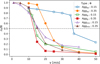 |
Fig. 6 Normalised number of particles within the final largest fragment (nf/N) as function of the collision velocity, v. |
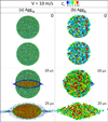 |
Fig. 7 Central sections of thickness 14 Rg showing the temporal evolution of a collision for (a) Aggsg with ϕ=0.15 and (b) Agglg with ϕ= 0.15. The colour scale shows the coordination for each grain. |
3.4 Coordination
The coordination Ci is the number of contacts that each grain i has. Two grains are considered to be in contact if they exhibit a non-zero overlap δ (Eq. (A.1)). The total number of contacts in an aggregate is then ∑ Ci/2 and the mean coordination is given by
 (4)
which represents the average number of contacts per grain for an aggregate composed of Ng grains. Table 7 presents the initial mean coordination 〈C〉0 for all samples shown in Figure 1. Only a slight variation in 〈C〉0 is observed, despite the fact that the samples are constructed with significantly different filling factors (ϕ=0.15 and ϕ=0.35). This is a result of the aggregate assembly method, which is detailed in Section 2.1.
(4)
which represents the average number of contacts per grain for an aggregate composed of Ng grains. Table 7 presents the initial mean coordination 〈C〉0 for all samples shown in Figure 1. Only a slight variation in 〈C〉0 is observed, despite the fact that the samples are constructed with significantly different filling factors (ϕ=0.15 and ϕ=0.35). This is a result of the aggregate assembly method, which is detailed in Section 2.1.
During the simulations, grains break existing contacts and form new ones, causing Ci to vary and, consequently, altering the mean coordination 〈C〉. This evolution is illustrated in Figure 7a for case 1 and in Figure 7b for case 3, both corresponding to simulations conducted with a collision velocity of v = 10 m s−1 and filling factor of ϕ=0.15. The colour scale represents the coordination Ci of each individual grain i. Red corresponds to coordination values of 4 or higher. Figure 7 displays central slices to visualise the variation in Ci towards the centre of the aggregates. These slices have a thickness of 14 Rg, which corresponds to 7 μ m in Figure 7a and 35 μ m in Figure 7b.
In Figure 7a, we examined case 1 (Aggsg and ϕ=0.15). Initially (t=0), the grains have different Ci values, but the distribution is homogeneous throughout the aggregates, with no uncoordinated grains (there are no grains with Ci=0). As the aggregates come into contact, a shock wave characterised by uncoordinated grains is generated and propagated from the collision zone toward the edge of the aggregates. At t=10 μ s this wave is visible in blue (indicating Ci=0), behind a central region where Ci is higher, predominantly displaying values of 3, 4, or greater. By t=25 μ s, the wave reaches the extremes, and a more compact central region is observed: a remnant denser than the initial aggregate. The thickness of this wave of uncoordinated grains is defined as the distance between the innermost and outermost grains of the wave, while the shock propagation speed is defined as the average rate at which the wave position changes over time. For the case shown in Figure 7a, the average wave thickness and propagation speed are 2.7 μ m and 1.75 m s−1, respectively. These propagation waves in uncoordinated grains may depend, in addition to monomer size and sample porosity, on the material composition of the monomers. Studies of low-velocity collisions between more compact aggregates composed of smaller ice monomers do not appear to display this trend (Arakawa et al. 2024). Future investigations considering variations in both monomer size and material could provide a more comprehensive understanding of this behaviour. Ejecta grains are mostly monomers or small fragments, as discussed in Section 3.2.
In Figure 7b, the shock wave is less evident than in Figure 7a, with only a small number of uncoordinated grains (in blue) at 10 μ s. These few grains barely appear to form a shock front similar to that observed in Figure 7a. This effect is primarily due to the lower number of grains in the aggregates (see Table 4). However, compaction is also achieved, and the remnant observed at 25 μ s exhibits grains with higher coordination, resulting in an increase in 〈C〉 by the end of the simulation.
The effect shown in Figure 7 is common to all collisions performed between monodisperse aggregates (cases 1-4). In general, it is found that for collisions between aggregates of type Aggsg, there is a well-defined wave of uncoordinated grains that propagates from the moment the aggregates collide. This generates a rearrangement of the monomers with compaction, as the smaller grains have more space to reorganise. The most porous samples facilitate this process even more, which is in line with previous studies (Planes et al. 2020). On the other hand, collisions between aggregates of type Agglg are hindered by the size of the monomers, making rearrangement more difficult. It is important to recall that the fragmentation velocity for aggregates of type Aggsg is higher than for Agglg aggregates, which is directly correlated with the fact that smaller monomer size allows for easier compaction and consequently greater fracture resistance.
Figure 8 presents a collision at v = 10 m s−1 and ϕ=0.15 with aggregates Aggmix (case 5), illustrating the evolution of the coordination of the grains. The colour scale shows the coordination value of each grain. A central slice with a thickness of 12 μ m was taken. Initially, the majority of the small grains (radius Rsg) have an initial coordination Ci less than 4, while large grains (radius Rlg), colored in red, exhibit much higher coordination values, exceeding 4, with a maximum value of Ci=68, as a large grain can make simultaneous contacts with many small grains. In Figure 8, coordination values are shown up to 4 to emphasise the change in the coordination of the small grains. At t= 10 μ s, the aggregates come into contact, and an effect similar to the one previously shown in Figure 7a is again observed. There is a shock wave marked in blue with uncoordinated small grains (radius Rsg) travelling from the centre to the ends, but lacking a shape as symmetrical as in the case of Figure 7a. This is due to the presence of large grains that are not uncoordinated, since they have a large number of contacts maintained from the beginning, mainly with small grains, making it very difficult for them to be completely isolated from the rest of the sample. Also, a central section showing an increase in coordination is generated. At t= 25 μ s, the wave reaches the extremes, and grains and fragments are ejected. The observed fragments are generally composed of a few large grains, accompanied by many small ones.
To perform a more quantitative analysis, we examined the temporal evolution of the mean coordination 〈C〉 for v = 10 m s−1, where all cases lead to coagulation. We did the same for v= 40 m s−1, where all cases lead to fragmentation (see Table 6).
Figure 9a shows the variation of 〈C〉 for all samples at v = 10 m s−1, a velocity at which no fracture occurs. We denote 〈C〉f as the final mean coordination, which represents the value at which 〈C〉 stabilises by the end of the simulation. A similar behaviour is observed for the six cases. The initial values, 〈C〉0, at t=0 are shown in Table 7; all are close to 2. When the aggregates come into contact, 〈C〉 decreases, since, as seen in Figures 7 and 8, a shock wave is generated composed of uncoordinated grains (with a null C value). After reaching a minimum, 〈C〉 begins to grow because in the central region the coordination of the grains increases. Then, 〈C〉 reaches its maximum value 〈C〉f and stabilises as interactions between the grains cease. For all cases where the collision velocity was 10 m s−1, an increase in the final value of 〈C〉f with respect to the initial value is observed. If we consider the filling factor of ϕ=0.15, we see that the highest value is reached in case 1(Aggsg), followed by case 5(Aggmix) and finally by case 3(Agglg). We observe that, in general, the order of the curves follows the trend according to which the grain radius determines the highest value of 〈C〉 reached. Similarly, for samples with a filling factor of ϕ=0.35, the same pattern is observed. These results appear to follow the same trend as those obtained for the fragmentation velocity of the aggregates (see Section 3.3). This was expected based on the results from the previous sections and further confirms the relevance of monomer size in the outcomes.
All curves for cases with ϕ=0.15 show a steeper slope before reaching their minimum, whereas the curves for cases with ϕ= 0.35 exhibit a much less pronounced slope, or are virtually flat, as seen in case 4 (red curve in Figure 9a. This may be due to the higher number of uncoordinated grains, which is a result of the larger void volume in the more porous samples (lower ϕ). Additionally, for samples with a higher filling factor (ϕ=0.35), the increase in 〈C〉 is faster (the maximum is reached in less time compared to the more porous analogue samples), likely due to the reduced capacity for grain rearrangement.
On the other hand, the analysis of Figure 6 pointed out that the filling factor, ϕ, was also decisive for samples of type Aggsg, but not so relevant in the other cases. Case 1(Aggsg and ϕ=0.15) showed a different behaviour from the rest and greater resistance to fragmentation. If the behaviour of this case (blue curve in Figure 9a) is compared with case 5 (violet curve), it can be seen that both start with a similar initial mean coordination, but later, for case 1, the minimum in 〈C〉 is higher and reaches a higher 〈C〉f than case 5. In percentage terms, 〈C〉 increases by 39% for case 1 and only 24% for case 5. A possible explanation is that, in case 5, the presence of even a small number of particles with Rlg=2.5 μ m, due to their large size, acts as a barrier hindering the growth of the average number of contacts.
It is worth noting that cases 3 and 4, shown in Fig. 9a, begin and end with approximately equal values of 〈C〉 despite their different porosities. However, case 4 differs from all the other cases by presenting a smoother curve where the minimum is barely perceptible. This suggests that even with large monodisperse monomers, a high filling factor prevents particle miscoordination. This highlights that while porosity does not affect the final outcome for the aggregate type Agglg, it plays an important role in understanding the physical processes involved in the dynamics of any collisional event.
Figure 9b illustrates the evolution of 〈C〉 for v = 40 m s−1, where fragmentation occurs for all cases. The behaviour differs between the six cases, and the main determining factor is the radius of the monomers.
Cases 1 and 2 in Fig. 9b show an evolution similar to that obtained for the velocity v = 10 m s−1, with a drop in 〈C〉 at the beginning of the simulation and its subsequent increase, obtaining maximum values at the end of the simulation. This first drop in 〈C〉 is associated with the uncoordination of many grains at the time of impact and the consequent wave propagation of grains with C=0. These simulations with collisions between aggregates of type Aggsg are the only ones that report a net increase in 〈C〉 for this velocity, even though they fragment after the collision. This occurs because the final fragments, although smaller than the initial aggregates, are more compact, with a greater number of contacts between grains. Although the final value 〈C〉f is similar for both, as they start from a different initial value, it is worth noting that the case with the highest percentage increase in its average coordination is case 1(22%) compared to case 2 (13%).
For cases 3 and 4 of Fig. 9b (Agglg), there is an initial drop in 〈C〉, followed by a gradual increase after 5 μ s, but overall a net decrease in 〈C〉(〈C〉f. less than 〈C〉0). The filling factor does not seem to affect the evolution of the 〈C〉f values obtained for these cases, with percentage drops of 12% and 13% for cases 3 and 4, respectively. The size of the monomer is again identified as the key factor influencing the final variation of 〈C〉. Specifically, for aggregates composed of large monomers (radius Rlg), 〈C〉 decreases, whereas for aggregates composed of smaller monomers (radius Rsg), 〈C〉 increases.
For cases 5 and 6 of Fig. 9b (Aggmix), a distinct behaviour characterised by peaks is observed: after an initial decrease in 〈C〉, the value momentarily rises at times t=3.75 μ s and 2.5 μ s, respectively. Since this effect was observed only for Aggmix, it is speculated that it is due to the differential monomer radius. These abrupt growths can be explained considering that large grains (radius Rlg) act as barriers, causing many small grains (radius Rsg) to adhere to them in a short time. This effect is momentary, as the subsequent lack of coordination of the small grains causes the mean coordination of the samples to drop rapidly until reaching a minimum, after which it begins to grow until stabilising at 〈C〉f. It is observed that cases 5 and 6 (Aggmix) in both Figs. 9a and 9b exhibit a final coordination number relative to the initial one that is higher for ϕ=0.35 than for ϕ= 0.15. This is consistent with previous studies on bidisperse samples conducted by Umstätter & Urbassek (2021a), who found that, at higher initial filling factors, the fragments reach higher coordination numbers.
Thus, the observed behaviours highlight the complex interactions between grain size, coordination, and porosity in the evolution of the samples during collisions. The appearance of transient peaks in 〈C〉 for bidisperse grain aggregates suggests that the combination of small and large grains introduces additional dynamics not seen in monodisperse grain aggregates. These results further reinforce the importance of considering the monomer size distribution when analysing the fragmentation dynamics in granular systems. Studying these collisions is relevant for understanding the early stages of protoplanetary disk evolution, where such interactions play a significant role in dust coagulation and the initial stages of planetary formation.
Initial average coordination for the six samples.
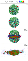 |
Fig. 8 Central sections of thickness 12 μ m showing the temporal evolution of a collision for case 5(Aggmix and ϕ=0.15). The colour scale shows the coordination for each grain. |
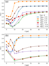 |
Fig. 9 Time evolution of the mean coordination of the six cases with: (a) v = 10 m s−1, where all outcomes are adhesion, (b) v = 40 m s−1, where all outcomes are fragmentation. The values of the final mean coordination number 〈C〉f for each case are reported in the same order as the legend (from top to bottom): (a) 3.03, 3.29, 2.69, 2.68, 2.72, 3.02; (b) 2.66,2.76,1.8,1.81,2.0, and 2.25. |
4 Conclusions and future outlook
We used numerical simulations to recreate dust-dust collisions between micrometric amorphous silica aggregates. This study offers insights into how monomer size and distribution influence fragmentation and coagulation processes. We conducted simulations with bimodal or mixed monomer size samples, which improve the representation of dust in protoplanetary environments and set a precedent for their broader use in collision studies. These samples exhibit distinct behaviours compared to monodisperse aggregates, highlighting the importance of considering porosity and monomer size distribution when modelling dust evolution. In this work, we developed a software tool and used it to efficiently track the fragmentation dynamics of these aggregates throughout the simulations.
The simulations show that collision velocity and monomer size are the main drivers of fragmentation. Higher velocities increase fragmentation and aggregates composed of smaller grains resist breaking due to their larger number of contacts, leading to steeper fragment distributions. Porosity plays a secondary role, enhancing resistance in aggregates with small grains, whereas larger grains hinder reorganisation. Mixed aggregates behave in between, but even a small fraction of large grains strongly affects the outcome. The results emphasise that monomer size distribution and porosity significantly impact aggregate growth and fragmentation, shaping the conditions under which pebbles form. Since pebbles are essential building blocks in planetesimal and planet formation, understanding their formation mechanisms contributes to refining planetary formation models.
Collisions in protoplanetary disks generally involve a range of impact parameters. Head-on collisions represent an idealised subset of the full collisional dynamics. Previous studies have shown that the outcomes of offset collisions can differ significantly from head-on cases with critical disruption velocities that could be largely independent of aggregate size in the presence of an impact parameter (Wada et al. 2009). While our current study focuses on head-on collisions to isolate the collisional behaviour due to the different monomer sizes and configurations, it would be important in future works to explore collisions with varying impact parameters. This would enable us to obtain a better understanding of more realistic scenarios of aggregate growth and fragmentation in protoplanetary environments.
In future work, we aim to investigate samples with a broader range of monomer sizes to better replicate the size distributions observed in the studied environments. Additionally, we plan to study samples with more values of porosity to gain a deeper understanding of the underlying dependencies. An interesting avenue for further research would be to explore the barrier effect of larger grains, which is expected to play a significant role in the coordination evolution of mixed samples. One approach could involve generating coordination histograms at different time intervals and performing coordination analyses that distinguish between different monomer sizes.
Acknowledgements
FP, MBP, ENM, and MGP acknowledge support from SIIPUNCuyo grant 80020240100348 UN. We thank Herbert Urbassek for valuable discussions. This work used the Toko Cluster from FCEN, UNCuyo, which is part of the SNCAD, MinCyT, Argentina.
Appendix A Granular model
Granular aggregates consist of monomers, also referred to as grains, which are indivisible spherical particles. All the grains that form the aggregate must be in contact with at least one other grain. The overlap of two individual grains is denoted as:
 (A.1)
where 1/R*=1/R1+1/R2 (Ri is the radius of the grain i=1, 2) and r12 is the distance between their centres. The normal force between two grains consists of:
(A.1)
where 1/R*=1/R1+1/R2 (Ri is the radius of the grain i=1, 2) and r12 is the distance between their centres. The normal force between two grains consists of:
a repulsive part described by the Hertzian δ3/2 law, based on elasticity theory for isotropic materials (Pöschel & Schwager 2005), which is given by
 (A.2)
where E* represents the effective elastic modulus:
(A.2)
where E* represents the effective elastic modulus:  , being Yi the Young’s modulus and vi is the Poisson’s ratio for the grains i=1,2. If the grains have the same material composition, Y1=Y2=Y and v1=v2=v. The normal direction is indicated by n̂=r12/‖r12‖.
an attractive contribution Fadh, which is taken to be proportional to the specific surface energy γ. Different models related Fadh with γ. In this work, we use the JKR model (Johnson et al. 1971), in which the short-range surface forces act only within the contact area, expressed as
 (A.3)
where a is the radius of the contact zone, related to the overlap δ according to
(A.3)
where a is the radius of the contact zone, related to the overlap δ according to  .
.
For the construction of our aggregates, each grain must be attached to another at its equilibrium distance, d0, following
 (A.4)
which is obtained by equating FHertz (Eq. A.2) and Fadh (Eq. A.3). Then, the corresponding equilibrium overlap δ0 between two grains in contact is
(A.4)
which is obtained by equating FHertz (Eq. A.2) and Fadh (Eq. A.3). Then, the corresponding equilibrium overlap δ0 between two grains in contact is
![Mathematical equation: $\delta_{0}=\sqrt[3]{3 R^{*}}\left(\frac{\pi \gamma}{E^{*}}\right)^{2 / 3}.$](/articles/aa/full_html/2025/11/aa56240-25/aa56240-25-eq14.png) (A.5)
(A.5)
After constructing the aggregates, we modelled their subsequent dynamical interaction, incorporating both normal and tangential frictional forces, which depend on the type of motion between two grains. The normal direction experiences viscoelastic dissipation, while the tangential forces include sliding friction, rolling friction, and torsional (twisting) friction. For sliding motion, the frictional force is characterised by parameters such as the shear modulus and the radius of the contact area. In contrast, rolling motion is hindered by a torque that prevents the grains from freely rotating over each other, governed by a specific distance over which they can move without breaking atomic contacts. Additionally, torsional motion experiences resistance through a torque that depends on the material properties and the size of the contact area, further hindering the grains’ rotation. For more details on the calculation of the forces, we refer to Ringl & Urbassek (2012); Dominik & Tielens (1997).
Appendix B Graph-based method
A graph is a way of organising information using points, called nodes, and lines that connect them, called edges (Bollobás 2013). They are used to represent relationships and connections in various fields, such as computer science, engineering, and social sciences. For example, they can model transportation networks, electrical circuits, relationships between people, or even structures in biology. Granular materials have been studied using graphs, and extensively within the framework of network science (Papadopoulos et al. 2018).
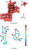 |
Fig. B.1 Two fragments of case 3 (Rg=2.5 μ m, ϕ=0.15). In (a), the Ovito visualisation, and in (b), its representation as a graph coloured by the coordination, Ci. |
Two methods were used to obtain the fragments after the collisions. For the monodisperse samples (cases 1−4 in Table 4), the Ovito software (Stukowski 2010) was used with the coordination analysis modifier, which calculates the coordination number of each grain by counting the number of neighbouring particles within a specified cutoff distance. For the bidisperse samples (cases 5 and 6, Table 4), we developed software that uses graphs to calculate the coordination and cluster analysis of these samples.
For both types of analysis, a cutoff distance is specified, and the following is obtained:
cluster analysis: groups monomers according to contacts where each cluster represents a fragment;
coordination analysis: returns the coordination of each grain, namely, the number of contacts it has with other grains.
To obtain the coordination of each grain, its distance from all the other grains is calculated. Then, it is evaluated whether these distances are equal to the equilibrium distance, d0, which depends on the radius of the grains and is specified in Table 3 for each case. The contacts are counted, and the information is saved. For the analysis of fragments, the generated code performs the aforementioned procedure. Then, a graph of the sample is generated using the Python library NetworkX (Aric A. Hagberg & Swart 2008). This graph-based tool allows the calculation of the coordination Ci for each grain i in the mixed samples.
Figure B.1 shows the graph obtained for two fragments resulting from the collision at v=30 m s−1 for case 3 of Table 4. Figure B.1(a) shows the fragments in perspective, but all grains are of the same size. Figure B.1(b) displays the graph projected onto a plane, where each node (grain) is coloured according to its degree. This degree represents the coordination Ci (see Section 3.4). The edges (connections) of the graph represent contacts between grains that are at the equilibrium distance, d0.
References
- Akiba, Y., Wang, S., Sato, M., & Shima, H., 2023, J. Phys. Soc. Jpn., 92, 104801 [Google Scholar]
- Arakawa, S., Tanaka, H., & Kokubo, E., 2022, ApJ, 933, 144 [NASA ADS] [CrossRef] [Google Scholar]
- Arakawa, S., Okuzumi, S., Tatsuuma, M., et al. 2023, ApJ, 951, L16 [NASA ADS] [CrossRef] [Google Scholar]
- Arakawa, S., Tanaka, H., Kokubo, E., Nishiura, D., & Furuichi, M., 2023, A&A, 670, L21 [NASA ADS] [CrossRef] [EDP Sciences] [Google Scholar]
- Arakawa, S., Tanaka, H., Kokubo, E., et al. 2024, Granular Matter, 26, 92 [Google Scholar]
- Aric A. Hagberg, D. A. S., & Swart, P. J., 2008, Proceedings of the 7th Python in Science Conference (SciPy2008), 11 [Google Scholar]
- Bandyopadhyay, R., & Urbassek, H. M., 2023, Sci. Rep., 13, 2072 [Google Scholar]
- Beitz, E., Güttler, C., Blum, J., et al. 2011, ApJ, 736, 34 [NASA ADS] [CrossRef] [Google Scholar]
- Beitz, E., Blum, J., Parisi, M. G., & Trigo-Rodriguez, J., 2016, ApJ, 824, 12 [Google Scholar]
- Bentley, M. S., Arends, H., Butler, B., et al. 2016, Acta Astronaut., 125, 11 [NASA ADS] [CrossRef] [Google Scholar]
- Birnstiel, T., Klahr, H., & Ercolano, B., 2012, A&A, 539, A148 [NASA ADS] [CrossRef] [EDP Sciences] [Google Scholar]
- Biswas, S., Goehring, L., & Chakrabarti, B. K., 2019, Statistical Physics of Fracture and Earthquakes [Google Scholar]
- Blum, J., 2018, Space Sci. Rev., 214, 52 [NASA ADS] [CrossRef] [Google Scholar]
- Blum, J., & Münch, M., 1993, Icarus, 106, 151 [Google Scholar]
- Blum, J., & Wurm, G., 2008, Annu. Rev. Astron. Astrophys., 46, 21 [CrossRef] [Google Scholar]
- Bollobás, B., 2013, Modern Graph Theory, 184 (Springer Science & Business Media) [Google Scholar]
- Carballido, A., Cuzzi, J. N., & Hogan, R. C., 2010, MNRAS, 405, 2339 [NASA ADS] [Google Scholar]
- Carrasco-González, C., Sierra, A., Flock, M., et al. 2019, ApJ, 883, 71 [Google Scholar]
- Chokshi, A., Tielens, A., & Hollenbach, D., 1993, ApJ, 407, 806 [NASA ADS] [CrossRef] [Google Scholar]
- Doi, K., & Kataoka, A., 2023, ApJ, 957, 11 [CrossRef] [Google Scholar]
- Dominik, C., & Tielens, A., 1997, ApJ, 480, 647 [NASA ADS] [CrossRef] [Google Scholar]
- Dominik, C., Blum, J., Cuzzi, J. N., & Wurm, G., 2007, in Protostars and Planets V, eds. B. Reipurth, D. Jewitt, & K. Keil, 783 [Google Scholar]
- Estrada, N., 2016, Phys. Rev. E, 94, 062903 [Google Scholar]
- Estrada, P. R., Cuzzi, J. N., & Umurhan, O. M., 2022, ApJ, 936, 42 [NASA ADS] [CrossRef] [Google Scholar]
- Ginski, C., Tazaki, R., Dominik, C., & Stolker, T., 2023, ApJ, 953, 92 [NASA ADS] [CrossRef] [Google Scholar]
- Gunkelmann, N., Ringl, C., & Urbassek, H. M., 2016, A&A, 589, A30 [NASA ADS] [CrossRef] [EDP Sciences] [Google Scholar]
- Güttler, C., Blum, J., Zsom, A., Ormel, C. W., & Dullemond, C. P., 2010, A&A, 513, A56 [Google Scholar]
- Güttler, C., Mannel, T., Rotundi, A., et al. 2019, A&A, 630, A24 [NASA ADS] [CrossRef] [EDP Sciences] [Google Scholar]
- Hasegawa, Y., Suzuki, T. K., Tanaka, H., Kobayashi, H., & Wada, K., 2023, ApJ, 944, 38 [NASA ADS] [CrossRef] [Google Scholar]
- Hilchenbach, M., Kissel, J., Langevin, Y., et al. 2016, ApJ, 816, L32 [CrossRef] [Google Scholar]
- Hyodo, R., Ida, S., & Guillot, T., 2021, A&A, 645, L9 [NASA ADS] [CrossRef] [EDP Sciences] [Google Scholar]
- Ishii, T., & Matsushita, M., 1992, J. Phys. Soc. Jpn., 61, 3474 [Google Scholar]
- Johnson, K. L., Kendall, K., & Roberts, A. D., 1971, Proc. Roy. Soc. Lond. A Math. Phys. Sci., 324, 301 [Google Scholar]
- Jutzi, M., Michel, P., Benz, W., & Richardson, D. C., 2010, Icarus, 207, 54 [Google Scholar]
- Kimura, H., Wada, K., Senshu, H., & Kobayashi, H., 2015, ApJ, 812, 67 [NASA ADS] [CrossRef] [Google Scholar]
- Kobayashi, N., & Shibayama, H., 2021, J. Phys. Soc. Jpn., 90, 124002 [Google Scholar]
- Kolokolova, L., Lara, L., Schulz, R., Stüwe, J., & Tozzi, G., 2003, JQSRT, 79, 861 [Google Scholar]
- Krijt, S., Ormel, C. W., Dominik, C., & Tielens, A. G., 2015, A&A, 574, A83 [NASA ADS] [CrossRef] [EDP Sciences] [Google Scholar]
- Kun, F., Pál, G., Varga, I., & Main, I. G., 2019, Philos. Trans. Roy. Soc. A, 377, 20170393 [Google Scholar]
- Lasue, J., Levasseur-Regourd, A. C., Hadamcik, E., & Alcouffe, G., 2009, Icarus, 199, 129 [NASA ADS] [CrossRef] [Google Scholar]
- Macías, E., Espaillat, C. C., Osorio, M., et al. 2019, ApJ, 881, 159 [CrossRef] [Google Scholar]
- Meisner, T., Wurm, G., Teiser, J., & Schywek, M., 2013, A&A, 559, A123 [NASA ADS] [CrossRef] [EDP Sciences] [Google Scholar]
- Millán, E. N., Planes, M. B., Bringa, E. M., & Parisi, M. G., 2025, Granular Matter, 27, 3 [Google Scholar]
- Oquendo-Patiño, W. F., & Estrada, N., 2020, Granular Matter, 22, 1 [CrossRef] [Google Scholar]
- Ormel, C., Spaans, M., & Tielens, A., 2007, A&A, 461, 215 [NASA ADS] [CrossRef] [EDP Sciences] [Google Scholar]
- Oshiro, H., Tatsuuma, M., Okuzumi, S., & Tanaka, H., 2025, ApJ, 983, 75 [Google Scholar]
- Pabst, W., & Gregorová, E., 2013, Ceram. Silikaty, 57, 167 [Google Scholar]
- Papadopoulos, L., Porter, M. A., Daniels, K. E., & Bassett, D. S., 2018, J. Complex Networks, 6, 485 [Google Scholar]
- Paszun, D., & Dominik, C., 2009, A&A, 507, 1023 [NASA ADS] [CrossRef] [EDP Sciences] [Google Scholar]
- Planes, M. B., Millán, E. N., Urbassek, H. M., & Bringa, E. M., 2019, MNRAS, 487, L13 [CrossRef] [Google Scholar]
- Planes, M. B., Millán, E. N., Urbassek, H. M., & Bringa, E. M., 2020, MNRAS, 492, 1937 [NASA ADS] [CrossRef] [Google Scholar]
- Planes, M. B., Millán, E. N., Urbassek, H. M., & Bringa, E. M., 2021, MNRAS, 503, 1717 [CrossRef] [Google Scholar]
- Planes, M. B., Parisi, M. G., Millán, E. N., Bringa, E. M., & Cañada-Assandri, M., 2024, MNRAS, 531, 3168 [Google Scholar]
- Pöschel, T., & Schwager, T., 2005, Computational Granular Dynamics: Models and Algorithms (Springer Science & Business Media) [Google Scholar]
- Pueyo, S., 2011, Landscape Ecol., 26, 305 [Google Scholar]
- Ringl, C., & Urbassek, H. M., 2012, Comput. Phys. Commun., 183, 986 [NASA ADS] [CrossRef] [Google Scholar]
- Ringl, C., Bringa, E. M., Bertoldi, D. S., & Urbassek, H. M., 2012, ApJ, 752, 151 [NASA ADS] [CrossRef] [Google Scholar]
- Sierra, A., Pérez, L. M., Zhang, K., et al. 2021, ApJS, 257, 14 [NASA ADS] [CrossRef] [Google Scholar]
- Stukowski, A., 2010, Modelling and Simulation in Materials Science and Engineering, 18 [Google Scholar]
- Teiser, J., & Wurm, G., 2009, MNRAS, 393, 1584 [NASA ADS] [CrossRef] [Google Scholar]
- Testi, L., Birnstiel, T., Ricci, L., et al. 2014, Protostars and Planets VI, 339 [Google Scholar]
- Thompson, A. P., Aktulga, H. M., Berger, R., et al. 2022, Comput. Phys. Commun., 271, 108171 [CrossRef] [Google Scholar]
- Trilling, D. E., Lisse, C., Cruikshank, D. P., et al. 2020, Nat. Astron., 4, 940 [Google Scholar]
- Umstätter, P., & Urbassek, H. M. 2021a, A&A, 652, A40 [NASA ADS] [CrossRef] [EDP Sciences] [Google Scholar]
- Umstätter, P., & Urbassek, H. M. 2021b, Granular Matter, 23, 33 [CrossRef] [Google Scholar]
- Umstätter, P., Gunkelmann, N., Dullemond, C. P., & Urbassek, H. M., 2019, MNRAS, 483, 4938 [NASA ADS] [Google Scholar]
- Wada, K., Tanaka, H., Suyama, T., Kimura, H., & Yamamoto, T., 2008, ApJ, 677, 1296 [NASA ADS] [CrossRef] [Google Scholar]
- Wada, K., Tanaka, H., Suyama, T., Kimura, H., & Yamamoto, T., 2009, ApJ, 702, 1490 [Google Scholar]
- Wada, K., Tanaka, H., Okuzumi, S., et al. 2013, A&A, 559, A62 [NASA ADS] [CrossRef] [EDP Sciences] [Google Scholar]
- Weidenschilling, S., & Cuzzi, J. N., 1993, in Protostars and Planets III, 1031 [Google Scholar]
- Weidenschilling, S. J., 1997, in Astronomical Society of the Pacific Conference Series, 122, From Stardust to Planetesimals, ed. Y. J. Pendleton, 281 [Google Scholar]
- Weidling, R., Güttler, C., Blum, J., & Brauer, F., 2009, ApJ, 696, 2036 [NASA ADS] [CrossRef] [Google Scholar]
- Wurm, G., & Teiser, J., 2021, Nat. Rev. Phys., 3, 405 [CrossRef] [Google Scholar]
- Zhang, S., Zhu, Z., Ueda, T., et al. 2023, ApJ, 953, 96 [NASA ADS] [CrossRef] [Google Scholar]
- Zhu, Z., & Yang, C.-C., 2021, MNRAS, 501, 467 [Google Scholar]
- Zsom, A., Ormel, C. W., Güttler, C., Blum, J., & Dullemond, C. P., 2010, A&A, 513, A57 [NASA ADS] [CrossRef] [EDP Sciences] [Google Scholar]
The filling factor ϕ is called global packing fraction in Millán et al. (2025) (see their Table 1).
All Tables
All Figures
|
Fig. 1 Global view of each aggregate type with ϕ=0.15 and ϕ=0.35. Blue and pink grains correspond to Rg=0.5 μ m and Rg=2.5 μ m, respectively. Numbers refer to the cases listed in Table 4. |
| In the text | |
|
Fig. 2 Temporal evolution of a collision between aggregates composed of identical grains. (a) Simulation of case 2: Rg=Rsg=0.5 μ m with ϕ=0.35. (b) Simulation of case 4: Rg=Rlg=2.5 μ m with ϕ=0.35. The colour-coding indicates the magnitude of the velocity vi of each particle. |
| In the text | |
|
Fig. 3 Temporal evolution of a collision with v = 10 m s−1 between aggregates composed of bidisperse grains. Simulation of case 6: Rsg = 0.5 μ m and Rlg=2.5 μ m with ϕ=0.35. The colour-coding indicates the magnitude of the velocity vi of each particle. |
| In the text | |
|
Fig. 4 Fragment distribution, F(n), for simulations with a collision velocity of v = 10 m s−1. |
| In the text | |
|
Fig. 5 Fragment distribution F(n) for simulations with collision velocity v = 40 m s−1. |
| In the text | |
|
Fig. 6 Normalised number of particles within the final largest fragment (nf/N) as function of the collision velocity, v. |
| In the text | |
|
Fig. 7 Central sections of thickness 14 Rg showing the temporal evolution of a collision for (a) Aggsg with ϕ=0.15 and (b) Agglg with ϕ= 0.15. The colour scale shows the coordination for each grain. |
| In the text | |
|
Fig. 8 Central sections of thickness 12 μ m showing the temporal evolution of a collision for case 5(Aggmix and ϕ=0.15). The colour scale shows the coordination for each grain. |
| In the text | |
|
Fig. 9 Time evolution of the mean coordination of the six cases with: (a) v = 10 m s−1, where all outcomes are adhesion, (b) v = 40 m s−1, where all outcomes are fragmentation. The values of the final mean coordination number 〈C〉f for each case are reported in the same order as the legend (from top to bottom): (a) 3.03, 3.29, 2.69, 2.68, 2.72, 3.02; (b) 2.66,2.76,1.8,1.81,2.0, and 2.25. |
| In the text | |
|
Fig. B.1 Two fragments of case 3 (Rg=2.5 μ m, ϕ=0.15). In (a), the Ovito visualisation, and in (b), its representation as a graph coloured by the coordination, Ci. |
| In the text | |
Current usage metrics show cumulative count of Article Views (full-text article views including HTML views, PDF and ePub downloads, according to the available data) and Abstracts Views on Vision4Press platform.
Data correspond to usage on the plateform after 2015. The current usage metrics is available 48-96 hours after online publication and is updated daily on week days.
Initial download of the metrics may take a while.