| Issue |
A&A
Volume 703, November 2025
|
|
|---|---|---|
| Article Number | A88 | |
| Number of page(s) | 6 | |
| Section | Cosmology (including clusters of galaxies) | |
| DOI | https://doi.org/10.1051/0004-6361/202556337 | |
| Published online | 07 November 2025 | |
Cosmological implications of the Gaia Milky Way declining rotation curve
1
École Centrale de Lyon, 36 Avenue Guy de Collongue, 69134 Écully, France
2
Université de Toulouse, UPS-OMP, IRAP, CNRS, 14 Avenue Edouard Belin, F-31400 Toulouse, France
⋆ Corresponding authors: This email address is being protected from spambots. You need JavaScript enabled to view it.
; This email address is being protected from spambots. You need JavaScript enabled to view it.
Received:
9
July
2025
Accepted:
19
September
2025
Abstract
Although the existence of dark matter has been widely acknowledged in the cosmology community, its nature remains unknown despite decades of research. This calls into questions its very existence. This never-ending search for dark matter has led us to consider alternatives. Since increasing the enclosed mass is the only way to explain the flat appearance of galaxies’ rotation curves in a Newtonian framework, modified Newtonian dynamics (MOND) theory proposes a modification to Newton’s dynamics when the acceleration of matter at given radius is around or below a threshold value, a0. Observed rotation curves, generally flat at large distances, are then usually well reproduced by MOND with an a0 of ∼1.2 × 10⁻¹⁰ m/s2. However, recent Gaia evidence indicates a decline in the Milky Way rotation curve, which a distinct behavior. Therefore, we examine whether MOND can accommodate the Gaia declining rotation curve of the Milky Way. We first use a standard model to describe the Milky Way’s baryonic components. Secondly, we show that a Navarro, Frenk, and White model is able to fit the decline, assuming a scale radius (Rs) on the order of 4 kpc. In a third step, we show that the usual MOND paradigm is not able to reproduce the declining part in a standard baryonic model. Finally, we examine whether the MOND theory can accommodate the declining part of the rotation curve when the characteristics of the baryonic components are relaxed. To do so, we used a Markov chain Monte Carlo method to determine the characteristics of the stellar and HI disks, including their masses, that would result in the best possible fit of the decline. We find that the stellar disk should be massive, on the order of 1011 M⊙. The HI disk mass is capped at nearly 1.8 × 10¹¹ M⊙ but could also be negligible. Finally, a0 is consistent with 0, with an upper limit of 0.53 × 10⁻¹⁰ m/s2 (95%), a value much lower than that usually advocated to explain standard flat rotation curves in MOND theory (∼1.2 × 10⁻¹⁰ m/s2).
Key words: Galaxy: kinematics and dynamics / dark matter
© The Authors 2025
 Open Access article, published by EDP Sciences, under the terms of the Creative Commons Attribution License (https://creativecommons.org/licenses/by/4.0), which permits unrestricted use, distribution, and reproduction in any medium, provided the original work is properly cited.
This article is published in open access under the Subscribe to Open model. This email address is being protected from spambots. You need JavaScript enabled to view it. to support open access publication.
1. Introduction
Studying galaxies’ rotation curves (RCs) is of paramount importance in cosmology, as they hint at the existence of dark matter. Observations have shown that most galaxies’ RCs are flat, which is in strong disagreement with Newtonian dynamics’ predictions for known baryonic components. Historically, cosmologists’ favorite answer to this crisis is to assume the existence of an invisible mass in order to accommodate the observations. This assumption is also supported by the observations of unrelated phenomena, including gravitational lensing (Refregier 2003) and the cosmological microwave background (Ade et al. 2016). Dark matter, whose quantity was estimated to be nearly 30% of the Universe’s mass-energy content, has now become a pillar of cosmology’s standard model, Λ cold dark matter (ΛCDM).
However, since dark matter has never been observed directly, we could alternatively envisage that Newtonian dynamics changes under certain conditions. Modified Newtonian dynamics (MOND) theory (Milgrom 1983) proposes a modification of Newtonian dynamics in regimes where the acceleration approaches or drops below a characteristic value of the acceleration, a0. In the deep MOND limit, the rotation velocity of a circular orbit resumes to v = (GMa0)1/4, which explains the flat appearance of most RCs. Previous fits of RCs using MOND agree on a value of about 1.2 × 10⁻¹⁰ m/s2 (Begeman et al. 1991), an acceleration threshold so low that MONDian effects could not be detected on Earth nor in the Solar System. This theory has been further developed, leading to more complex formulations such as AQUAL (Bekenstein & Milgrom 1984), QUMOND (Milgrom 2023), or the relativistic TeVeS (Bekenstein 2004). However, these theories face tensions in multiple fields, such as galaxy cluster dynamics (Sanders 2003), cosmological microwave background anisotropies, and difficulties to fit the matter power spectrum (Dodelson 2011). To alleviate these tensions, hybrid theories have been put forward (see for example Bruneton et al. 2009 or Skordis & Złośnik 2021 for ΛCDM cosmology with MONDian effects at galactic scales). Despite those tensions, MOND remains a simple theory for reproducing flat galaxies’ RCs. However, according to a statistical analysis of galaxy RCs from Spitzer Photometry and Accurate Rotation Curves (SPARC), the agreement does not favor MOND (Khelashvili et al. 2024).
Although it is relatively easy to measure other galaxies’ RCs (Corbelli & Salucci 2000; Roberts 1975), probing the Milky Way’s from the inside is a challenge at high radii. Available data tend to confirm that the MW’s RC is flat (Mroz et al. 2019), consistent with both dark matter and MOND. However, some moderate decline has been reported (Robin et al. 2022), in agreement with an earlier claim consistent with the radial acceleration relation (McGaugh 2019). A moderate decline was also inferred for the most luminous galaxies (Persic et al. 1996; Salucci et al. 2007). However, Gaia’s latest data release (Vallenari et al. 2022) sheds light on a velocity decline after ≈15 kpc, on the order of 3.5 km/s/kpc, which different analyses agree on (see for example Wang et al. 2022; Zhou et al. 2023; Jiao et al. 2023; Ou et al. 2024). This decline is also consistent with previous indications for the presence of a dip in the Milky Way’s RC (Huang et al. 2016) with a higher significance level. Some other galaxies’ RCs were also found to be declining: a sample of 22 galaxies was studied under the MOND paradigm by Zobnina & Zasov (2020). They conclude that some galaxies’ RCs do not align with the usual MOND paradigm, needing a value of a0 lower than values obtained from previous fits of the RCs. Studying Gaia’s newfound decline might yield similar conclusions regarding the Milky Way. Milky Way RC measurements before the decline are nonetheless more scattered; different papers have found very different values (e.g. Iocco et al. 2015; Mroz et al. 2019; Zhou et al. 2023; Sylos Labini et al. 2023; Wang et al. 2022; McGaugh 2018; Robin et al. 2022). Such considerations led us to focus on the declining part of the RC without considering the inner part.
In this study we aim to shed light on the declining RC’s implications regarding MOND as inferred from Gaia, without attempting to fit the inner part. We started by building a model for the baryonic components of the Milky Way in order to compute the RC at various radii from the Galactic center. To compare ΛCDM with MOND, we implemented this model both under a dark matter paradigm and under Milgrom’s modified dynamics. We then used this model as a basis to find the optimal value of a0 that fits the decline – if such a value exists. Finally, we compared MOND results with ΛCDM, and we detail why the MOND paradigm does not accommodate the Milky Way RC under reasonable assumptions. This interpretation of the data is based on the assumption of simple dynamics that are not violently disturbed in the outer parts of the Galaxy (Koop et al. 2024; Kroupa et al. 2024).
2. The Milky Way’s rotation curve
2.1. Modeling the baryonic components of the Milky Way
In order to compute the RC, we first need to establish a model for the spatial distributions of the baryonic components of the Milky Way. We chose to work with the B2 model used in Jiao et al. (2023) and described in de Salas et al. (2019). This model consists of three components: (i) a spherical bulge modeled by a Hernquist potential,
 (1)
(1)
(ii) a thin stellar disk, and (iii) multiple gas disks. Given the values provided by de Salas et al. (2019) and references therein, we only considered the HI disk since the other gas masses are negligible.
Both the stellar disk and the HI disk densities are given by a double exponential,
 (2)
(2)
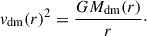
where i ∈ {st., HI} and ρ0i is a normalization constant:
We used the Mi, Mbulge, rdi, zdi, Rt, and rb values from de Salas et al. (2019), which are listed in Table 1.
B2 model parameters (de Salas et al. 2019).
The stellar population of the Galaxy can be described by more complex models with several different components. The presence of a thick disk, for instance, impacts the vertical structure of the velocity dispersion as well as the possible flaring of the disk (López-Corredoira 2025). To determine what the presence of a thick disk would imply, we also computed the circular velocity in a model comprising two equal-mass components (Pouliasis et al. 2017), one in a thin disk and one in a thick disk, following the Miyamoto–Nagai profile (Miyamoto & Nagai 1975). From Figs. 1 and 2, one can see that the RCs are nearly identical. Concerning the flaring, we note that Sylos Labini (2024) conclude that its impact has only a marginal effect on the RC at large distances, i.e., at the scales relevant to our study. In our work the RC is examined at a distance far from the bulk of the stellar components.
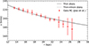 |
Fig. 1. RC decline example using NFW with ρ0,NFW = 1.8 × 10⁸ M⊙/kpc3, Rsthin = 3.97 kpc, and Rsthin + thick = 3.98 kpc. The parameters for the baryonic components are those of the B2 model in Table 1 taken from Jiao et al. (2023). We also provide the RC (gray lines) with two disks, one thin and one thick (see Sect. 2.1). |
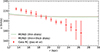 |
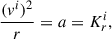
Fig. 2. Decline fit under the MOND paradigm. a0thin = 2.417 × 10⁻¹⁰ m/s2, and a0thin + thick = 2.429 × 10⁻¹⁰ m/s2. The parameters for the baryonic components are the same as in Fig. 1. |
2.2. Rotation curve under ΛCDM
In Newtonian dynamics, assuming a circular movement, each mass component produces an acceleration field that can be written in terms of a circular velocity associated with this component:
 (3)
(3)
where a is the radial acceleration, Kri is the total radial force per unit mass, and i corresponds to any baryonic component described above (stellar disk, bulge, or gas disk) or to the added dark matter mass component: i ∈ {st.,bulge, HI,dm}.
This means that in order to compute the velocity, we first have to determine the radial force. We did so by integrating Poisson’s equation with the density ρi. For the density given in Eq. (2), Poisson’s equation can be solved in terms of Hankel transforms. We can thus find the radial force by considering the R derivative. Details of calculation can be found in Kuijken & Gilmore (1989). We can easily determine vbulge using Eq. (3) and the first derivative of Hernquist’s potential, Eq. (1).
Finally, we need to specify a dark matter model to compute vdm. In ΛCDM, dark matter potentials are expected to follow a Navarro, Frenk, and White (NFW) profile (Navarro et al. 1996). We therefore used a standard NFW model (Navarro et al. 1996):
 (4)
(4)
where ρ0,NFW and the scale radius (Rs) are free parameters. Then we only needed to integrate the density of Eq. (4) between 0 and a given radius (r) to get the enclosed mass in the corresponding sphere, and then used the circular movement assumption to obtain the velocity:
The RC under a circular movement assumption can now be evaluated:
 (5)
(5)
Using Eq. (5), we can now compute the RC under the ΛCDM dark matter paradigm. We provide an example in Fig. 1, with parameters chosen to yield an acceptable fit to the declining part of the RC. This example shows that NFW is able to accommodate the declining part, with a χ2 of χthin2 = 2.6, χthin + thick2 = 3.1 (reduced χ of 0.2 and 0.24), which is low but acceptable.
This yields different results than Jiao et al. (2023). When computing the dynamical mass using the same critical density value as Jiao et al. (2023) using the parameters from our fit of the RC under NFW, we get Mdyn = 4.28 × 10¹¹ M⊙ for a virial radius of 153.5 kpc. These values are higher than the results from Jiao et al. (2023) and consistent with Sylos Labini (2024). They are also consistent with their newfound upper limit on the dynamical mass. In addition, extrapolation to a distance nearly ten times greater is highly uncertain: on galaxy scales, strong feedback is expected (Blanchard et al. 1992), which could seriously alter the dark matter distribution in the inner part of galaxies (Li et al. 2022). The concentration parameter (c) for the above characteristics is larger than found by Eilers et al. (2019), but our fit is performed only on R > 13 kpc. Our value of c is much larger than the average value expected from ΛCDM simulations involving only dark matter (Bullock et al. 2001). The role of baryons may, however, considerably increase the concentration parameter on galaxy scales (Shao et al. 2023). We note that Lin & Li (2019) infer a determination of the Milky Way’s RC up to 100 kpc, consistent with a NFW profile, with data roughly consistent with those used in Fig. 1, although not reproduced by the global fit that covers the RC in the range 4.6 − 98 kpc from Huang et al. (2016). Finally, we note that dynamical arguments from the stellar streams dynamics (Ibata et al. 2024) as well as from the local group kinematics (Benisty 2024) point consistently toward a Milky Way mass on the order of or above 1012 M⊙.
2.3. Rotation velocity under MOND
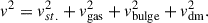
Using the standard MOND formulation instead of a more rigorous one in a RC computation leads to a difference of about 5% (López-Corredoira & Betancort-Rijo 2021). For the sake of simplicity, we thus stuck to Newton’s second law as modified in Milgrom (2015):
 (6)
(6)
where a is the acceleration that now may differ from the total radial force per unit mass (Kr), and μ is a function chosen such that (McGaugh 2004)
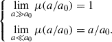
We chose to work with  , as it is standard and was used by McGaugh (2004)1. By only keeping the a > 0 solution, one can derive the total velocity from Eq. (6):
We then fit the declining part of the RC with this MOND paradigm under the baryonic models described above. The value of a0 was determined by minimizing the χ2 and considering the Jiao et al. (2023) declining part of the RC. The best value of a0 found here is 2.417 × 10⁻¹⁰ m/s2, which is not consistent with the value derived from the RC in other galaxies. The resulting RC is shown in Fig. 2. The corresponding χ2, 49.7 and 57.6 (reduced χ2 of 3.83 and 4.43), confirm the visual impression that the fits are not satisfying. We thus conclude that using the B2 model described in Jiao et al. (2023), both with thin and thick disks, the declining RC cannot be reproduced with Milgrom dynamics. The physical reason for the behavior of the RC can be understood: the bulk of the mass is within 13 kpc, and the mass beyond 13 kpc is so low that the dynamic is in the MONDian regime and the RC is nearly flat.
3. Relaxing the baryonic components to fit the decline with MOND
3.1. Methodology
We have seen that MOND theory cannot accommodate the declining part of the RC of the Milky Way when the baryonic components are those of the B2 model as presented in Sect. 2.1. In this section we examine whether relaxing the properties of the baryonic components could alleviate this inconsistency. As the disk mass is the dominant baryonic component, it is clearly an important parameter in the Milky Way RC. We thus treated this quantity as a free parameter, as well as a0. For the scale radius, we used two values: rd = 2.35 kpc (which is the value measured by Misiriotis et al. 2006 and used by both Jiao et al. 2023 and de Salas et al. 2019) and rd = 3.1 kpc, which are close to the bounds provided by Bland-Hawthorn & Gerhard (2016).
To determine our two parameters, the disk mass (Mst.) and a0, we ran two Markov chain Monte Carlo (MCMC) analyses, one for each scale radius. We applied the MCMC ensemble slice sampler algorithm from ZEUS (Karamanis et al. 2021). Mst. was allowed to vary between 3 × 10¹⁰ M⊙ and 2 × 10¹¹ M⊙ and a0 between 0 and 3 × 10⁻¹⁰ m/s2.
3.2. Results
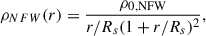
Applying the methodology described above yields constraints on the parameter space (see Fig. 3). The uncertainty on Mst. is representative of the extreme values found in Binney & Tremaine (2011) and Bland-Hawthorn & Gerhard (2016), and the uncertainty on a0 can be found in Milgrom (2015). One can see that there is a correlation between the stellar disk mass and a0. Moreover, the value of rd does not have much of an impact on the results. From these contours we extracted the pair of values (Mst., a0) presented in Table 2 that minimizes the χ2: χ2 = 5.53 for rd = 2.35 kpc, and χ2 = 3.84 for rd = 3.1 kpc; these values are slightly higher than with NFW but still acceptable considering we only have two free parameters (see Fig. 4).
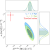 |
Fig. 3. MCMC contours for rd = 2.35 kpc and rd = 3.1 kpc. The stellar disk mass and a0 are left as free parameters. The red cross indicates the observed values of Mstellar and the standard value of a0 with their respective uncertainty (see the main text). |
Central values for rd = 2.35 kpc and rd = 3.1 kpc.
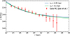 |
Fig. 4. Fits using MCMC results (Table 2). The parameters for the other baryonic components are the same as in Fig. 2. |
The obtained value of a0 is smaller than the standard 1.2 × 10⁻¹⁰ m/s2 and is not consistent with previous results, namely from Begeman et al. (1991). In other words, according to our study, there is no way for MOND to explain both the Milky Way RC and other galaxies’ RCs with the same value of a0. A similar conclusion is obtained by Chan & Law (2023).
Moreover, the stellar disk mass used to find such a value is about 10 × 1010 solar masses, which is not consistent with the value (3.5 ± 1)×1010 M⊙ from Bland-Hawthorn & Gerhard (2016). The physical reason is that in order to produce a decreasing RC at r> 15 kpc, the dynamic needs to be close to the Newtonian regime, which in turn requires a high mass (more than 95‰ of the mass lies within a radius of 15 kpc). The MONDian regime starts at a larger radius with a value of a0 lower than the standard value.
3.3. More freedom on the baryonic components
Since relieving constraints on the stellar disk mass alone does not yield satisfying results, in this section we explore possibilities by increasing the number of free parameters on the baryonic components. We launched another MCMC run with Mst., a0, MHI, rd, and zd as free parameters. Each prior used for this MCMC can be found in Table 3.
A number of interesting properties can be inferred from Fig. 5: it is possible to adequately fit the RC with the baryonic components provided that they are allowed to take values well above the standard values: for the models taken in the 1σ domain, the χ2 typically lies between 3 and 6, which is acceptable and similar to the ΛCDM case. The scale height of the disk has no correlation with other parameters (except a weak correlation with the disk mass) and has no preferred value. The HI disk mass (MHI) has little to no impact on the results; a wide range of values allowed us to fit the decline. High HI disk masses are allowed, far above the standard value but still below the preferred stellar disk mass. The 1σ intervals for the scale radius of the stellar disk and for its mass are higher than found in Bland-Hawthorn & Gerhard (2016) and show a correlation with the stellar disk mass. Relieving the constraints on the baryonic matter distribution yields a lower value for a0 than found in the previous MCMC analysis, and a0 does not appear to be correlated with the baryonic distribution parameters. One can see that a0 = 0 m/s2 is in the 1σ interval, assuming a heavy stellar disk and a scale radius (rd) > 3 kpc. The fact that the stellar disk is heavier than usual observations (Bland-Hawthorn & Gerhard 2016) can be explained by the close-to-zero value of a0: since little to no MONDian effect is required and no dark halo is assumed, one needs extra matter in the disk to reach an acceptable value of the circular velocity. Essentially, this consists in a dark matter disk instead of the halo used in Fig. 1, and models using a lighter disk and a nonvanishing a0 are not significantly preferred over the a0 = 0 paradigm.
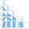 |
Fig. 5. MCMC contours with a free stellar disk mass, free HI disk mass, free a0, free scale radius, and free scale height. |
4. Discussion and conclusion
In this work we examined the two major solutions to the missing mass problem in galaxies, applied to the Milky Way. More precisely, we compared the ability of ΛCDM and MOND to fit the Milky Way’s declining RC measured by Gaia, assuming a simple dynamic that is not significantly disturbed in the outer parts of the Galaxy (Koop et al. 2024; Kroupa et al. 2024). Using a standard model for the baryonic components of the Milky Way, we show that a simple dark matter distribution model like NFW, expected in ΛCDM, is able to explain Gaia’s decline with ease, albeit with an extreme value for the concentration parameter. On the other hand, the MOND formulation cannot accommodate the decline under the B2 model, even when allowing a0 to be a free parameter. We then considered relieving constraints on baryonic parameters as well as the value of a0 in order to examine whether MOND could accommodate the decline. For this we performed an MCMC analysis on a0 and the parameters of the baryonic components using the data of the declining part of the Milky Way RC. Preferred models have disk masses at odds with values inferred from observations, with no significant preference for a nonvanishing a0. We get an upper limit on a0 of 0.53 × 10⁻¹⁰ m/s−2 (95%), which is significantly lower (by 5σ) than what has been found necessary to fit flat RCs in other galaxies with MOND.
We conclude that the declining RC of the Milky Way as recently inferred from Gaia data can be interpreted as being due to the presence of an NFW-type dark matter halo. It is not easy to reproduce in the MOND alternative.
This choice is not important as we focus on the asymptotic behavior of the curve. We have verified that the flattening of the RC is similar to the so-called simple function (Famaey & Binney 2005).
Acknowledgments
This work was supported by the Programme National Cosmology et Galaxies (PNCG) of CNRS/INSU with INP and IN2P3, co-funded by CEA and CNES. This work was supported by CNES.
References
- Ade, P. A. R., Aghanim, N., Arnaud, M., et al. 2016, A&A, 594, A13 [NASA ADS] [CrossRef] [EDP Sciences] [Google Scholar]
- Begeman, K. G., Broeils, A. H., & Sanders, R. H. 1991, MNRAS, 249, 523 [Google Scholar]
- Bekenstein, J. D. 2004, Phys. Rev. D, 70, 083509 [Google Scholar]
- Bekenstein, J., & Milgrom, M. 1984, ApJ, 286, 7 [NASA ADS] [CrossRef] [Google Scholar]
- Benisty, D. 2024, A&A, 689, L1 [NASA ADS] [CrossRef] [EDP Sciences] [Google Scholar]
- Binney, J., & Tremaine, S. 2011, Galactic Dynamics Second Edition (Princeton University Press) [Google Scholar]
- Blanchard, A., Valls-Gabaud, D., & Mamon, G. A. 1992, A&A, 264, 365 [NASA ADS] [Google Scholar]
- Bland-Hawthorn, J., & Gerhard, O. 2016, ARA&A, 54, 529 [Google Scholar]
- Bruneton, J.-P., Liberati, S., Sindoni, L., & Famaey, B. 2009, JCAP, 2009, 021 [Google Scholar]
- Bullock, J. S., Kolatt, T. S., Sigad, Y., et al. 2001, MNRAS, 321, 559 [Google Scholar]
- Chan, M. H., & Law, K. C. 2023, ApJ, 957, 24 [Google Scholar]
- Corbelli, E., & Salucci, P. 2000, MNRAS, 311, 441 [NASA ADS] [CrossRef] [Google Scholar]
- de Salas, P. F., Malhan, K., Freese, K., Hattori, K., & Valluri, M. 2019, JCAP, 2019, 037 [Google Scholar]
- Dodelson, S. 2011, Int. J. Mod. Phys. D, 20, 2749 [NASA ADS] [CrossRef] [Google Scholar]
- Eilers, A.-C., Hogg, D. W., Rix, H.-W., & Ness, M. K. 2019, ApJ, 871, 120 [Google Scholar]
- Famaey, B., & Binney, J. 2005, MNRAS, 363, 603 [NASA ADS] [CrossRef] [Google Scholar]
- Huang, Y., Liu, X. W., Yuan, H. B., et al. 2016, MNRAS, 463, 2623 [CrossRef] [Google Scholar]
- Ibata, R., Malhan, K., Tenachi, W., et al. 2024, ApJ, 967, 89 [NASA ADS] [CrossRef] [Google Scholar]
- Iocco, F., Pato, M., & Bertone, G. 2015, Nat. Phys., 11, 245 [NASA ADS] [CrossRef] [Google Scholar]
- Jiao, Y., Hammer, F., Wang, H., et al. 2023, A&A, 678, A208 [NASA ADS] [CrossRef] [EDP Sciences] [Google Scholar]
- Karamanis, M., Beutler, F., & Peacock, J. A. 2021, MNRAS, 508, 3589 [NASA ADS] [CrossRef] [Google Scholar]
- Khelashvili, M., Rudakovskyi, A., & Hossenfelder, S. 2024, ArXiv e-prints [arXiv:2401.10202] [Google Scholar]
- Koop, O., Antoja, T., Helmi, A., Callingham, T. M., & Laporte, C. F. P. 2024, A&A, 692, A50 [NASA ADS] [CrossRef] [EDP Sciences] [Google Scholar]
- Kroupa, P., Pflamm-Altenburg, J., Mazurenko, S., et al. 2024, ApJ, 970, 94 [NASA ADS] [CrossRef] [Google Scholar]
- Kuijken, K., & Gilmore, G. 1989, MNRAS, 239, 571 [NASA ADS] [CrossRef] [Google Scholar]
- Li, P., McGaugh, S. S., Lelli, F., Schombert, J. M., & Pawlowski, M. S. 2022, A&A, 665, A143 [NASA ADS] [CrossRef] [EDP Sciences] [Google Scholar]
- Lin, H.-N., & Li, X. 2019, MNRAS, 487, 5679 [CrossRef] [Google Scholar]
- López-Corredoira, M. 2025, ApJ, 978, 45 [Google Scholar]
- López-Corredoira, M., & Betancort-Rijo, J. E. 2021, ApJ, 909, 137 [Google Scholar]
- McGaugh, S. S. 2004, ApJ, 609, 652 [NASA ADS] [CrossRef] [Google Scholar]
- McGaugh, S. S. 2018, RNAAS, 2, 156 [Google Scholar]
- McGaugh, S. S. 2019, ApJ, 885, 87 [Google Scholar]
- Milgrom, M. 1983, ApJ, 270, 365 [Google Scholar]
- Milgrom, M. 2015, Can. J. Phys., 93, 107 [NASA ADS] [CrossRef] [Google Scholar]
- Milgrom, M. 2023, Phys. Rev. D, 108, 084005 [NASA ADS] [CrossRef] [Google Scholar]
- Misiriotis, A., Xilouris, E. M., Papamastorakis, J., Boumis, P., & Goudis, C. D. 2006, A&A, 459, 113 [NASA ADS] [CrossRef] [EDP Sciences] [Google Scholar]
- Miyamoto, M., & Nagai, R. 1975, PASJ, 27, 533 [NASA ADS] [Google Scholar]
- Mroz, P., Udalski, A., Skowron, D. M., et al. 2019, ApJ, 870, L10 [Google Scholar]
- Navarro, J. F., Frenk, C. S., & White, S. D. M. 1996, ApJ, 462, 563 [Google Scholar]
- Ou, X., Eilers, A.-C., Necib, L., & Frebel, A. 2024, MNRAS, 528, 693 [NASA ADS] [CrossRef] [Google Scholar]
- Persic, M., Salucci, P., & Stel, F. 1996, MNRAS, 281, 27 [Google Scholar]
- Pouliasis, E., Di Matteo, P., & Haywood, M. 2017, A&A, 598, A66 [NASA ADS] [CrossRef] [EDP Sciences] [Google Scholar]
- Refregier, A. 2003, ARA&A, 41, 645 [NASA ADS] [CrossRef] [Google Scholar]
- Roberts, M. S. 1975, in Dynamics of the Solar Systems, ed. A. Hayli, IAU Symp., 69, 331 [Google Scholar]
- Robin, A. C., Bienaymé, O., Salomon, J. B., et al. 2022, A&A, 667, A98 [NASA ADS] [CrossRef] [EDP Sciences] [Google Scholar]
- Salucci, P., Lapi, A., Tonini, C., et al. 2007, MNRAS, 378, 41 [CrossRef] [Google Scholar]
- Sanders, R. H. 2003, MNRAS, 342, 901 [NASA ADS] [CrossRef] [Google Scholar]
- Shao, M. J., Anbajagane, D., & Chang, C. 2023, MNRAS, 523, 3258 [Google Scholar]
- Skordis, C., & Złośnik, T. 2021, Phys. Rev. Lett., 127, 161302 [NASA ADS] [CrossRef] [Google Scholar]
- Sylos Labini, F. 2024, ApJ, 976, 185 [CrossRef] [Google Scholar]
- Sylos Labini, F., Chrobáková, Ž., Capuzzo-Dolcetta, R., & López-Corredoira, M. 2023, ApJ, 945, 3 [NASA ADS] [CrossRef] [Google Scholar]
- Vallenari, A., Brown, A., & Prusti, T. 2022, A&A, 674, A1 [Google Scholar]
- Wang, H.-F., Chrobáková, Ž., López-Corredoira, M., & Sylos Labini, F. 2022, ApJ, 942, 12 [Google Scholar]
- Zhou, Y., Li, X., Huang, Y., & Zhang, H. 2023, ApJ, 946, 73 [CrossRef] [Google Scholar]
- Zobnina, D. I., & Zasov, A. V. 2020, Astron. Rep., 64, 295 [NASA ADS] [CrossRef] [Google Scholar]
All Tables
All Figures
|
Fig. 1. RC decline example using NFW with ρ0,NFW = 1.8 × 10⁸ M⊙/kpc3, Rsthin = 3.97 kpc, and Rsthin + thick = 3.98 kpc. The parameters for the baryonic components are those of the B2 model in Table 1 taken from Jiao et al. (2023). We also provide the RC (gray lines) with two disks, one thin and one thick (see Sect. 2.1). |
| In the text | |
|
Fig. 2. Decline fit under the MOND paradigm. a0thin = 2.417 × 10⁻¹⁰ m/s2, and a0thin + thick = 2.429 × 10⁻¹⁰ m/s2. The parameters for the baryonic components are the same as in Fig. 1. |
| In the text | |
|
Fig. 3. MCMC contours for rd = 2.35 kpc and rd = 3.1 kpc. The stellar disk mass and a0 are left as free parameters. The red cross indicates the observed values of Mstellar and the standard value of a0 with their respective uncertainty (see the main text). |
| In the text | |
|
Fig. 4. Fits using MCMC results (Table 2). The parameters for the other baryonic components are the same as in Fig. 2. |
| In the text | |
|
Fig. 5. MCMC contours with a free stellar disk mass, free HI disk mass, free a0, free scale radius, and free scale height. |
| In the text | |
Current usage metrics show cumulative count of Article Views (full-text article views including HTML views, PDF and ePub downloads, according to the available data) and Abstracts Views on Vision4Press platform.
Data correspond to usage on the plateform after 2015. The current usage metrics is available 48-96 hours after online publication and is updated daily on week days.
Initial download of the metrics may take a while.