| Issue |
A&A
Volume 703, November 2025
|
|
|---|---|---|
| Article Number | A188 | |
| Number of page(s) | 13 | |
| Section | Stellar atmospheres | |
| DOI | https://doi.org/10.1051/0004-6361/202556440 | |
| Published online | 13 November 2025 | |
Fluorescent Fe K line emission of γ Cas stars
II. Predictions for magnetic interactions and white-dwarf accretion scenarios
Space sciences, Technologies and Astrophysics Research (STAR) Institute, Université de Liège,
Allée du 6 Août, 19c, Bât B5c,
4000
Liège,
Belgium
★ Corresponding author: This email address is being protected from spambots. You need JavaScript enabled to view it.
Received:
16
July
2025
Accepted:
2
October
2025
Abstract
Context. About 12% of the early-type Be stars, which are not known X-ray binaries, exhibit an unusually hard and bright thermal X-ray emission. The X-ray emission of these so-called γ Cas stars could result from accretion onto a white dwarf companion or from magnetic interactions between the Be star and its decretion disc.
Aims. Exploring the full power of high-resolution X-ray spectroscopy of γ Cas stars requires the comparison of observations of the fluorescent Fe Kα emission lines near ~6.4keV with synthetic lines simulated for both scenarios.
Methods. We computed synthetic profiles of this line complex within the framework of the magnetic interaction and the accreting white dwarf scenarios. For the latter, we further distinguished between accretion onto a non-magnetic and a magnetic white dwarf. The various models account for different reservoirs of reprocessing material: the Be circumstellar decretion disc, the Be photosphere, an accretion disc around the putative white dwarf companion, a magnetically channelled accretion flow, and the white dwarf photosphere.
Results. We find considerably different line properties for the different scenarios. For a non-magnetic accreting white dwarf, the global Fe Kα complex is extremely broad, reaching a full width of 140 eV, whilst it is ~40 eV for the magnetic star–disc interaction and the magnetic accreting white dwarf cases. In the magnetic star-disc interaction, the line centroid is expected to follow the orbital motion of the Be star, whereas it should move along with the white dwarf in the case of an accreting white dwarf. For γ Cas, given the ~15× larger amplitude of the white dwarf orbital motion, the shift in position for an accreting white dwarf should be easily detectable with high-resolution spectrographs such as Resolve on XRISM, but remains essentially undetectable for the magnetic star-disc interaction.
Conclusions. Upcoming high-resolution spectroscopy of the fluorescent Fe Kα emission lines in the X-ray spectra of γ Cas stars will offer important insights into the properties of the primary X-ray source and of the illuminated material, allowing us to distinguish between the competing scenarios.
Key words: line: formation / line: profiles / stars: early-type / stars: emission-line, Be / X-rays: binaries / X-rays: stars
© The Authors 2025
 Open Access article, published by EDP Sciences, under the terms of the Creative Commons Attribution License (https://creativecommons.org/licenses/by/4.0), which permits unrestricted use, distribution, and reproduction in any medium, provided the original work is properly cited.
This article is published in open access under the Subscribe to Open model. This email address is being protected from spambots. You need JavaScript enabled to view it. to support open access publication.
1 Introduction
The star γ Cassiopeiae (HD 5394, B0.5 IVe) is well known as the prototype of classical Be stars, which are main-sequence or giant B-type stars that display or have displayed HI Balmer emission lines in their spectra (Rivinius et al. 2013). Half a century ago, the Small Astronomy Satellite (SAS-3) discovered a hard and moderately bright X-ray emission associated with γ Cas (Jernigan 1976; Mason et al. 1976). The properties of this X-ray emission, which is much brighter and harder than in the majority of Be stars but significantly fainter than in Be high-mass X-ray binaries (BeHMXBs), are a puzzle in stellar X-ray astrophysics (Smith et al. 2016; Nazé 2025). For a long time, γ Cas was the only object known to display these properties. However, over the past two decades, more than 30 Be stars with similar X-ray properties have been discovered (e.g. Smith & Balona 2006; Lopes de Oliveira et al. 2006; Nazé & Motch 2018; Nazé et al. 2020, 2022b; Nazé & Robrade 2023). Rather than an oddball, γ Cas is the prototype of a new class of objects, accounting for ~12% of the early-type Be stars (Nazé & Robrade 2023). The defining characteristics of these γ Cas stars are X-ray luminosities (in the 0.5–10keV band) ranging from LX ~ 4 × 1031 to 1.6 × 1033 erg s−1, log (LX / Lbol) between ~–6.2 and –4, and an X-ray emission arising in a thermal plasma with kT ≥ 5 keV (Nazé & Robrade 2023).
Observationally, γ Cas and a number of its comrades were found to be single-lined spectroscopic binary systems with orbital periods between weeks and months (Nazé et al. 2022a, and references therein). Existing orbital solutions allow for the unseen companions to be stripped helium subdwarfs1, white dwarfs (WDs), or neutron stars (NSs). The role of the compact companion in the generation of the peculiar X-ray emission remains currently debated. Indeed, the scenarios proposed to explain the X-ray emission can be divided into two broad categories: accretion onto a compact companion or magnetic star-disc interactions.
In the first category, ‘classical’ accretion onto a NS (White et al. 1982) as in BeHMXBs was excluded because of the thermal nature of the emission, its comparatively low luminosity, and the lack of X-ray pulsations and bursts (see e.g. Smith et al. 2016, and references therein). Postnov et al. (2017) proposed that the companion could be a rapidly spinning magnetic NS in the propeller regime with the rapid rotation of the magnetosphere prohibiting accretion. However, this scenario was refuted based on evolutionary as well as observational considerations (Smith et al. 2017; Rauw 2024). As an alternative to a NS, accretion onto a WD companion was put forth (e.g. Murakami et al. 1986; Hamaguchi et al. 2016; Tsujimoto et al. 2018, 2023; Gies et al. 2023; Toalá et al. 2025, and references therein). If this scenario were confirmed, γ Cas stars could populate the category of Be + WD systems predicted by binary evolution population synthesis models but which are currently largely under-represented in the observations (Shao & Li 2014).
The second category attributes the hard X-ray emission to interactions between the Be star and its decretion disc, without any direct intervention of the companion star. Motivated by observed correlations between X-ray and UV variability, which indicate that the two radiations arise close to each other, Smith et al. (1998) and Smith & Robinson (1999) elaborated the star-disc magnetic interaction scheme (see also Robinson & Smith 2000; Motch et al. 2015; Smith et al. 2016; Smith 2019). This scenario attributes the hard X-ray emission to magnetic reconnections between small-scale magnetic fields at the Be star surface, such as predicted by Cantiello & Braithwaite (2011), and a magnetic field rooted in the Be disc.
Whilst γ Cas stars have been observed with nearly every past or existing X-ray telescope, high-resolution X-ray spectroscopy of these objects, especially at energies between 6 and 7 keV, is still in its infancy. This energy range is especially relevant as it contains several emission lines with complementary diagnostic potentials. The He-like Fe XXV lines near 6.7 keV and the H-like Fe XXVI Lyα line at 6.97 keV provide information about the very hot plasma that makes up the primary source of hard X-rays. The fluorescent Fe Κα line near 6.4keV in turn probes the properties of both the primary hard X-ray source and the illuminated cool fluorescent material. Previous X-ray telescopes lacked the spectral resolution to resolve the details of those lines. Thanks to the Resolve X-ray microcalorimeters on board the X-ray and Imaging Spectroscopy Mission (XRISM, Ishisaki et al. 2022), this situation is changing as the first high-resolution spectra of γ Cas stars in this energy range are becoming available. Further progress will come with the X-ray Integral Field Unit (X-IFU, Peille et al. 2025) on the European Space Agency’s future Athena X-ray observatory.
Therefore, it is timely to investigate the diagnostic potential of the Fe Κα line in γ Cas stars. As a first step, Rauw (2024, hereafter Paper I) modelled the fluorescent line expected in the Postnov et al. (2017) propeller NS scenario. This study showed that the theoretical predictions could not be reconciled with the observed line strengths and absorbing column densities. In the present paper, we focus on the magnetic star-disc interaction and the accreting WD scenarios. Section 2 recalls the fundamental concepts of fluorescence, while Sect. 3 describes the circumstel-lar environment of the Be star and its putative WD companion. Fluorescent Fe Κα lines from the star-disc interaction scenario are discussed in Sect. 4, while Sect. 5 provides the results for accreting WDs. Finally, Sect. 6 presents our conclusions.
2 Modelling fluorescent emission
When a volume of relatively cool gas is illuminated by a bright and hard X-ray source, some atoms and ions in the gas undergo K-shell photoionisation by photons with energies exceeding that of the K-shell ionisation edge. Provided there remain electrons on the L- or M-shell, the ensuing vacancy on the K-shell is filled by one of these electrons. The excess energy of this electron is given away either via Auger autoionisation or by the emission of a fluorescent line photon. The probability that the process leads to fluorescent line emission instead of Auger autoionisation is called the fluorescent yield (e.g. Palmeri et al. 2003). The fact that Fe atoms and ions have relatively high fluorescent yields of about 0.3 (Kallman et al. 2004) makes the Fe Κα fluorescence line a rather prominent feature.
In γ Cas stars, several media provide reservoirs of cool material that can contribute to the fluorescent line emission. In the framework of the scenarios that we study here, these are the Be decretion disc, the Be photosphere, the circumstellar environment of the WD, and the WD atmosphere.
2.1 Fluorescence by circumstellar matter
Our approach to model the fluorescent emission from the cir-cumstellar material closely follows the method outlined in Paper I. The primary X-ray spectrum is described by an APEC optically thin thermal plasma model (Smith et al. 2001) extended by a bremsstrahlung continuum at energies above 100 keV. The energies of Fe Kα and Kβ lines as well as the branching ratios between those lines are taken from Yamaguchi et al. (2014) whilst fluorescent yields are from Kallman et al. (2004).
We briefly recall the main concepts of our method adopting the formalism for a point-like source of primary X-ray photons. Further details can be found in Paper I. The Fe Kα emissivity of a cell of material, of volume dV and hydrogen particle density nH(r), located at a position vector r from the centre of the Be star, and at a position d from the illuminating primary X-ray source can be written
 (1)
(1)
where σK–shell and Ethres are respectively the K-shell photoionisation cross section and the ionisation threshold energy, both evaluated according to Verner & Yakovlev (1995), EKα is the energy of the Kα line (Yamaguchi et al. 2014), zFe is the (solar) abundance of iron by number with respect to hydrogen (Asplund et al. 2009), xion is the relative abundance of a specific Fe ion, ωion+1 is the Kα fluorescent yield (Kallman et al. 2004), f (E, d) is the photon flux per unit energy at position d, and τ(Ε, d) is the optical depth along the line joining the cell to the primary X-ray source.
For an observer located in the direction n, the contribution of the cell of volume dV to the total line luminosity is expressed as
 (2)
(2)
where obs(r, n) is equal to 1 or 0 depending on whether or not the cell can be seen by the observer, and τ(ΕΚα, r, n) yields the optical depth at the energy of the Kα line integrated from the position r along the direction n.
2.2 Fluorescence in the stellar atmospheres
Some part of the hard X-rays illuminate the photosphere of either the Be star or the WD companion and could thus give rise to fluorescent line emission. Expressing the position inside the stellar atmosphere via the Rosseland optical depth, τRoss, the photosphere can be considered a semi-infinite medium illuminated from above by the primary X-ray source under an angle θin.
To represent the density structure inside the photospheres, we used the non-local thermodynamic equilibrium (nLTE) plane-parallel model atmosphere code TLUSTY (Hubeny & Lanz 2017a,b,c; Hubeny et al. 2021, and references therein). For the Be star, we used TLUSTY models from the BSTAR2006 grid of Lanz & Hubeny (2007). For the WD, we computed dedicated models with version 208 of TLUSTY (Hubeny et al. 2021). The optical depth for incoming X-rays of energy Ε is given by
 (3)
(3)
where σ(Ε) is the cross-section of the stellar material per H atom, and z stands for the geometrical position measured from the top of the photosphere (z < 0 inside the atmosphere). Using the TLUSTY tables, z can be converted into τROSS.
Here, we assume that we can treat the illuminating X-rays as a small perturbation that does not strongly alter the density, temperature and ionisation stratifications of the photosphere given by the TLUSTY models. To treat the radiative transfer, we adopt the Feautrier formalism of García & Kallman (2010). The mathematical details are outlined in Appendix A. The Feautrier equations are solved for a grid of values of μin = cos θin from 0.025 to 0.975. The stellar surface is discretised into 360 × 180 small cells. Depending on the geometry (point-like or extended) and location of the illuminating source of hard X-rays, and depending on the location of the observer, we evaluate for each of the cells the visibility of the source, the associated value of μin, and the value of μ = cos θ, where θ is the angle between the direction n towards the observer and the vertical z-axis. Moreover, the rotational velocity of each cell as seen by the observer is used to Doppler-shift the emerging fluorescent photon. All photons received by the observer are then grouped into a line profile according to their energy as seen by the observer.
2.3 Global Fe Κα profiles
As in Paper I, we first compute synthetic line profiles of individual transitions taking into account the Doppler shift due to the velocity component of the emitting cell along the n direction. The Κα line consists of an unresolved array of transitions arising from the various combinations of L and K shell electronic configurations (Palmeri et al. 2003). Each individual transition has its specific energy and intrinsic strength. The synthetic profiles of the full Fe Κα complex are then obtained by convolving the energy distribution of the transitions with the individual line profile weighted by the intrinsic strength of the transitions.
3 The circumstellar environment
To model the fluorescence from γ Cas, we need several parameters of the system. These include the spectral energy distribution of the primary X-ray emission, the orbital parameters of the binary system, the mass and radius of the Be star, and a description of the density structure of the circumstellar material. In Paper I, a set of relevant parameters was compiled. These default parameters are given in Table 1. Here, we added also our default parameters for the WD and its circumstellar environment.
The decretion discs of Be stars in low-eccentricity binary systems are usually expected to be truncated at the 3:1 resonance radius via gravitational interaction with the companion (Okazaki & Negueruela 2001; Okazaki et al. 2002; Panoglou et al. 2016). This concept has been revised in recent years, giving way to a more complex view of Be binary systems. Indeed, based on smoothed particle hydrodynamics (SPH) simulations, Martin et al. (2024) showed that in BeHMXBs the efficiency of tidal truncation depends on the disc aspect ratio. For H/R ≤ 0.1 tidal truncation was found to operate efficiently, but for larger H/R values its effect is much weaker. Since Be discs are flared, their aspect ratio increases with radius, which implies that disc truncation should be less efficient for longer period binaries which have wider orbital separations. Martin et al. (2024) further showed that material that escapes the Roche lobe of the Be star flows along tidal streams towards the compact companion’s gravitational sphere of influence where it forms an accretion disc. Similar conclusions were reached by Rubio et al. (2025) and Rast et al. (2025) who showed that instead of a sharp truncation, the density of the decretion disc undergoes a strong, azimuthally dependent decrease over a range of several stellar radii. Rubio et al. (2025) distinguished five regions in the Be binary system. With increasing distance from the Be star, these are (1) the inner Be disc, which is least perturbed by the companion, (2) a spiral-dominated disc featuring two-armed density waves, (3) a bridge formed by the denser arm that extends into the companion’s Roche lobe, (4) a disc-like accretion structure around the companion, and (5) a circumbinary envelope fed by material lost from the system. Figure 1 provides a sketch of the circumstellar environment of the Be star.
We assume that the innermost parts of the Be decretion disc can be described as an axisymmetric structure with a hydrogen number density distribution given by
![Mathematical equation: ${n_{\rm{H}}}\left( {r,z} \right) = {n_0}{\left( {{r \over {{R_*}}}} \right)^{ - \alpha }}\exp \left[ { - {1 \over 2}{{\left( {{z \over {H\left( r \right)}}} \right)}^2}} \right]$](/articles/aa/full_html/2025/11/aa56440-25/aa56440-25-eq6.png) (4)
(4)
(e.g. Hummel & Vrancken 2000). In this relation, r and z are the radial and vertical components of the cylindrical coordinates, n0 is the hydrogen number density at the inner edge of the disc, and H(r) is the disc scale height. The latter quantity varies with r as
 (5)
(5)
where cs(R*) is the speed of sound at the inner edge of the disc. The exponent p, introduced by Kurfürst et al. (2014) to describe the radial temperature profile of the disc, was taken to be p = 0.25. In the case of our default simulations for γ Cas, the aspect ratio remains below 0.1 all the way out to the 3:1 resonance radius (about 176 R⊙, Rauw et al. 2022), indicating that truncation might remain effective. The transition to an aspect ratio above 0.1 takes place at r = 194 R⊙.
To account for the more complex disc structure described by Rubio et al. (2025), we assumed the inner disc to extend out to 8 R* and represented the spiral dominated disc, the bridge region and the circumbinary region by two logarithmic spirals (see Fig. 1). To mimic the properties found by Rubio et al. (2025), both spirals were assumed to arise over a range in azimuthal angle of 30° and to have a density of 3 times the nominal density expected at this distance (as given by Eq. (4)). Conversely the inter-arm medium was assumed to have a density 0.6 times that given by Eq. (4). The spiral arms emanate from the disc at the points facing the secondary and opposite to it. The leading spiral arm, which turns into the bridge that connects with the secondary’s Roche lobe, stops at the position of the secondary, whilst the trailing arm feeds the circumbinary region (see Fig. 1). To avoid introducing additional parameters, we assume that the companion’s orbital plane coincides with the equatorial plane of the Be star, and hence the plane of the decretion disc.
Model parameters of γ Cas.
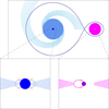 |
Fig. 1 Upper box: schematic pole-on view of the Be star (blue dot), its decretion disc and spiral extensions (sky blue), the WD companion, and its truncated accretion disc (magenta). The dark blue contour shows the Roche lobe of the system. The boxes at the bottom provide zooms on vertical cuts through the inner part of the Be decretion disc (left) and the surroundings of the WD (shown by the violet dot) with its magnetically truncated accretion disc (right). The red crosses correspond to the emitting regions of the primary X-rays. The left box illustrates the case of the magnetic star-disc interaction with magnetic field lines that connect the star and the disc. The right box corresponds to an accreting magnetic WD scenario where a magnetically channelled flow connects the truncated accretion disc to the magnetic poles of the WD. |
4 X-ray emission from the magnetic interaction scenario
In the context of the magnetic interaction scenario, the X-ray emission is attributed to magnetic reconnection events between localised magnetic fields at the surface of the Be star and magnetic fields arising inside the Be disc. The hot X-ray-emitting plasma would thus be located near the apex of the magnetic loops (Smith et al. 1998) in ‘canopies’ above the Be star and close to the innermost parts of the disc (Smith et al. 2016). To represent this situation, we consider two rings of material encircling the Be star, one above the equatorial decretion disc, the second one below the disc. In our default model, the rings are assumed to have a radius of Rs = 1.5 R* as measured from the Be star’s rotation axis, and to be located at a height Zs = 0.5 R* above or below the disc. In the absence of dedicated magneto-hydrodynamic simulations, these values were motivated by the constraint that, in this model, the primary X-ray emission arises near the Be star surface. The rings are discretised into 180 elements of 2° azimuthal extension. The total X-ray luminosity is distributed equally over those elements. Each element of the ring is assimilated to a point source, and the total fluorescent emission is obtained as the combination of the illumination by these 180 fake point sources.
This assumption implies that our model represents a time-averaged configuration. Indeed, at any given time, localised magnetic spots arising from the subsurface iron convection zone (Cantiello & Braithwaite 2011) are probably not distributed evenly in stellar longitude. Moreover, in the magnetic interaction scenario, the ubiquitous X-ray shots are interpreted as individual reconnection events taking place randomly, which implies a significant temporal variability of the X-ray emission from a specific element. Considering a typical ~50 ks integration time, needed to collect high-resolution X-ray spectra, we expect these rapid variations to average out.
As a first ingredient, we consider the fluorescent emission arising from the decretion disc. Because the illumination is maximum over the innermost parts of the disc, we start by assuming that the spiral part of the disc as well as the bridge and other components of the flow play only a minor role. The predicted individual line profile is shown in Fig. 2. The individual profile displays a double-peaked morphology reflecting the Keplerian velocity field of the inner disc part. The total equivalent width (EW) of the Be disc fluorescent line2 is predicted to be 49 eV whilst the line luminosity amounts to 3.3 × 1030 erg s−1. Part of the generated Fe Κα photons are reabsorbed by the disc material which is mildly optically thick in its inner regions3. Indeed, without this re-absorption, the EW would be 70 eV.
In our model of the magnetic interactions, the strength of the fluorescent line depends on the assumed location of the illuminating hot plasma ring. Figure 3 explores the dependence of the EW on the location of the extended primary source. If it is located very close to the Be star and to the decretion disc, it illuminates only a small part of the disc. Moreover, this part has the highest density and thus the highest optical depth for absorption of Fe Κα photons by the disc material. As a result, we expect the EW of the disc line to be relatively low. Moving to higher altitudes above the disc, that is increasing Zs, the illuminated part of the disc increases, but the ionising flux received by each cell of the disc decreases. Therefore, for Rs ≤ 1.3 R* and increasing Zs, the EW first increases before it decreases again. Finally, as Rs increases above 1.3 R*, those parts of the disc that are most strongly illuminated by the primary X-ray source are no longer optically thick and fully contribute to the strength of the fluorescence line. Over this part of the parameter space, where optical depth no longer plays a role, the EW is set by two competing trends. On the one hand, the density of the disc material, that most strongly contributes to the fluorescence, decreases with Rs, whereas, on the other hand, the extent of the illuminated region increases asymptotically with Rs. Hence, for a fixed Zs, EW increases as Rs increases from 1.3 R* up until ~2 R* and slowly decreases afterwards as the density of the most-strongly illuminated parts of the disc decreases.
We repeated the calculation of the line due to the Be disc, but this time accounting for the disc structure found by Rubio et al. (2025) according to our description above. The resulting individual line profile is compared with our simple disc model in Fig. 2. The two profiles are nearly identical as are the total EWs. This is because the bulk of the fluorescent emission arises from illumination of the inner part of the disc which is not impacted by the spiral structure. The observer’s viewing angle on the spiral arms (and thus their velocity along the observer’s sightline) changes as a function of orbital phase, which could lead to variations in the individual line profiles. However, because of their low density and large distance from the primary source, these arms contribute very little to the profile (see Fig. 2), and the ensuing variations should be very small.
Beside the Be disc, a second contribution to the fluorescent line comes from the illumination of the Be photosphere. Again the primary X-ray source was discretised into 180 small sectors, each one assimilated to a point source located at a distance  from the star’s centre. We then used the Feautrier method described in Appendix A in combination with a TLUSTY model atmosphere of solar metallicity, Teff = 25000 K, and log ɡ = 3.75, taken from the BSTAR2006 grid (Lanz & Hubeny 2007), to simulate the photospheric fluorescence.
In this model, the bulk of the photoelectric absorption by Fe ions, that is at the 7.1 keV K-shell ionisation edge, happen to occur at τRoss ≃ 1 (see Fig. 4). According to Fig. 16 of Lanz & Hubeny (2007), the dominant ionisation stage of Fe at these depths is Fe IV (≥90 %) with minor contributions from Fe III and Fe V (≤5 % for each of those species). We can use the ionisation parameter ξ, defined as
 (6)
(6)
with ne the electron density, and FX the X-ray flux over the 1–1000 Ry energy domain (Kallman et al. 2004), to assess the impact of the illumination by a powerful X-ray source on the ionisation balance. This impact is very small for log ξ < 0, but strongly increases for log ξ > 1 (see Fig. 6 of Kallman et al. 2004). At τRoss = 1, the electron density in the TLUSTY model is ≃4.6 × 1014 cm−3. For an extended source, with  , we obtain log ξ ≤ –5.1. Therefore, one does not expect significant changes of the ionisation of the photospheric material at the depths where most of the K-shell photoionisation takes place.
The predicted line profile is illustrated in Fig. 5. The total line luminosity from fluorescence in the Be photosphere amounts to 2.7 × 1027 erg s−1, and the EW to 0.05eV for Rs = 1.5 R* and Zs = 0.5 R*. This line strength is thus several orders below the disc contribution.
Accounting for the fact that the Fe Kα emission consists of a complex array of transitions, we convolved this array with the individual profiles obtained after summing the disc line and photospheric profiles. The result is illustrated in Fig. 6. We compare the synthetic profiles expected for the two quadrature orbital phases. The blue (resp. red) histogram yields the global Fe Kα fluorescent line profile with energy bins of 1 eV at the quadrature phase when the Be primary moves towards us (resp. away from us). We further convolved these synthetic profiles with an instrumental profile whose full width at half maximum (FWHM) would be equal to 5 eV. The results are shown in the bottom panel of Fig. 6. Owing to the widths of the individual profiles, the resulting blend does not allow one to distinguish the Kα1 and Kα2 subgroups. Kα2 only appears as an extension of the red wing of the blend. Moreover, with a semi-amplitude of 4.1 km s−1 (e.g. Rauw et al. 2022), the radial velocity (RV) motion of the Be star is too small to induce a measurable shift in the overall line profiles, even when considering the most extreme orbital phases.
The energy shift between the overall lines at those phases should be only ~0.2 eV.
At this stage, we thus conclude that the magnetic interaction scenario can reproduce the observed EWs of the fluorescent Fe Kα emission lines in γ Cas stars. An important observational test for this scenario stems from the fact that the line morphology should not vary in a systematic way with orbital phase of the companion and that the line centroid should not display significant RV variations.
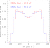 |
Fig. 2 Normalised individual Fe Κα line profile contributed by the Be decretion disc assuming an extended source represented by two rings of hot plasma of radius 1.5 R* and located 0.5 R* above or below the Be decretion disc. The line profile is binned into velocity bins of 50 km s−1 and is normalised by dividing by the total flux over the entire line profile. The spectral energy distribution of the illuminating source is an optically thin thermal plasma model with kT = 12.5 keV. The red histogram corresponds to an axisymmetric disc truncated at r = 176 R⊙. The blue histogram yields the results for a disc with spiral extensions as described in the text and computed out to a = 375 R⊙. The normalised profiles are displayed in velocity bins of 50 km s−1. |
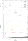 |
Fig. 3 Top: EW of the fluorescent Fe Κα line contributed by the Be decretion disc in the star-disc interaction scenario as a function of Rs for different values of Zs. Bottom: EW contours for the same scenario as a function of Rs and Zs. The primary source is modelled as a uniform axisymmetric ring of radius Rs from the polar axis of the Be star and of altitude Zs above the equatorial plane of the Be star. The hatched area in the bottom part corresponds to the scale height of the Be decretion disc. |
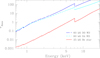 |
Fig. 4 Rosseland optical depth inside the photosphere where the optical depth for photoelectric absorption of X-rays reaches unity. The continuous red line illustrates the results for the Teff = 25 000 K, log ɡ = 3.75 TLUSTY model adopted for the Be star. The short-dashed cyan line and the long-dashed blue line correspond respectively to DA and DO WD models with Teff = 60 000 K and log ɡ = 8.5. |
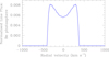 |
Fig. 5 Individual Fe Kα line profile contributed by the Be photosphere. The illuminating source is an extended ring-like source located at Rs = 1.5 R* and Zs = 0.5 R*. The spectral energy distribution of the illuminating source is an optically thin thermal plasma model with kT = 12.5 keV. |
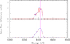 |
Fig. 6 Top: global line profile (i.e. combining the Be-disc and photo-spheric contributions and accounting for the full array of transitions) for our default magnetic interaction model, at two opposite quadrature orbital phases. The profiles are shown as histograms binned in energy bins of 1 eV. Bottom: convolution of the global line profiles with an instrumental response function of 5 eV FWHM. The magenta lines yield the theoretical energies of the centroids of the Fe V Kα1 and Kα2 subgroups (Palmeri et al. 2003) assuming Fe IV target ions. |
5 X-ray emission from accreting white dwarfs
Accreting WDs are found in two important categories of interacting binaries: cataclysmic variables (CVs) where the WD accretes material via Roche lobe overflow of a main-sequence low-mass star, and symbiotic stars where the mass donor is a red giant. X-ray emission of accreting WDs (for reviews see Mukai 2017; Page & Shaw 2022) is powered by accretion and/or nuclear fusion (either explosively, as in novae, or more steady). Nuclear burning at the surface of a WD manifests itself in the soft X-ray domain (below about 0.5 keV) as a so-called supersoft source. A few Be + WD systems have been identified in the SMC whilst they were undergoing an outburst (Kennea et al. 2021). These systems displayed bright (LX ≃ 1036 erg s−1 ) supersoft emission attributed to an enhanced accretion activity (rather than nuclear burning on the WD surface, Kennea et al. 2021). This situation differs significantly from γ Cas stars which rather exhibit a moderately bright, hard, and optically thin thermal X-ray emission that is more reminiscent of CVs in quiescence.
A key parameter of known accreting WDs is the strength of the WD’s magnetic field. If it is strong enough (>105 G, Page & Shaw 2022), the magnetic field takes control of the inflowing material which either entirely prevents the formation of an accretion disc or disrupts the accretion disc at the Alfvén radius of the WD, RA. Systems lacking an accretion disc are dubbed polars, whereas those with truncated discs are called intermediate polars (IPs). The former feature WDs with magnetic fields of about 7 × 10⁶–2 × 10⁸ G, whereas the latter have WD field strengths between 105 and 107 G (e.g. Ramsay & Cropper 2007). In such systems, the magnetically channelled accretion flow undergoes a hydrodynamic shock at some height, hs, above the WD surface near the magnetic poles. The hard primary X-ray emission arises in shock-heated plasma. The hardness of the corresponding emission depends directly on the WD mass (Mukai 2017). Frequently, this standoff shock is located close enough to the WD surface, typically at some fraction of the WD radius, RWD, so that the solid angle illuminated by the downward radiation is large (Hailey et al. 2016; Tsujimoto et al. 2018; Lopes de Oliveira & Mukai 2019). Assuming a point-like primary X-ray source, this solid angle is given by
 (7)
(7)
For low values of hs, the WD surface intercepts and reprocesses nearly half of the primary X-rays: they are either reflected, Compton scattered or absorbed to ionise iron atoms, resulting in fluorescent line emission. This allows for rather strong Fe Kα lines with EWs up to 100 and 200 eV in polars or IPs. By contrast, quiescent dwarf nova systems with low accretion rates (≤10−10 M⊙ yr−1) usually display weaker fluorescent lines (Ezuka & Ishida 1999; Pandel & Córdova 2005; Byckling et al. 2010; Eze 2015; Xu et al. 2016).
In this section, we consider the two scenarios, non-magnetic and magnetic WD in terms of the ensuing fluorescent Fe Kα line. Unfortunately, very little is known about the nature and properties of the companion of γ Cas. Assuming it to be a WD, its formation did not proceed along the path followed by classical WDs that are descendants of single low-mass stars. Instead, it would be the outcome of binary evolution, descending from a stripped hot subdwarf. Therefore, its temperature and chemical composition could differ from those of classical WDs. Similar uncertainties apply to the WD’s rotational velocity. In polars, one usually considers that the WD rotates synchronously with the orbital motion (e.g. Ramsay et al. 2001). Given the wide orbital separation and relative youth of γ Cas, synchronisation, which would imply a WD equatorial rotational velocity of 2.5 m s−1, is unlikely. From the observational viewpoint, several authors attempted to identify X-ray pulsation periodicities in the light curves of γ Cas stars that could reflect the rotational period of the putative WD companion. So far, no stable periodicity was found for γ Cas itself (Tsujimoto et al. 2018), but occasional transient signals have been reported for other γ Cas stars. For instance, Lopes de Oliveira et al. (2006) found an oscillation in the XMM-Newton light curve of HD 161103 with a period of about 3200 s, and Huenemoerder et al. (2024) reported a 3400 s periodicity in one Chandra observation of π Aqr. If these signals truly reflect the rotation of a WD companion, they would hint at low rotational velocities. In our calculations, we assumed  , corresponding to a rotation period of 1750 s. For the WD’s mass and radius, we adopted the parameters used by Rast et al. (2025): RWD = 0.01 R⊙, MWD = 0.98 M⊙. The SPH simulations carried out by Rast et al. (2025) predict an accretion rate of the WD in γ Cas of 2 × 10⁻¹¹ M⊙ yr−1, and we used this value as our baseline.
5.1 Accretion onto a non-magnetic WD
In non-magnetic CVs, accretion-powered X-rays are emitted in the boundary layer between the Keplerian accretion disc and the WD where the material slows down from a Keplerian rotation velocity near 3000 km s−1 to the significantly slower rotational velocity of the WD (Mukai 2017; Page & Shaw 2022). The hot gas then forms a hot corona with emission of X-rays up to 20 keV (Page & Shaw 2022).
For a non-magnetic WD secondary, the accretion disc extends from the radius of the WD’s Roche lobe down to the surface of the WD. We assimilated the primary X-ray source, that is the whole boundary layer, to a point-like source. To compute the fluorescence produced by an accretion disc illuminated by a compact object, we modified the code used in Sect. 4 by implementing a variable mesh step in the radial direction of the disc. This was necessary to account for the existence of two very different length scales which are RWD, and the orbital separation, a. In the innermost regions of the WD accretion disc, the radial step was set to 0.05 RWD and it was increased to 0.1 RWD (starting at r = 10 RWD), 1 RWD (starting at r = 100 RWD) and finally to  (starting at r = 500 RWD).
From dedicated SPH simulations of the γ Cas system, and assuming a WD nature of the secondary component, Rast et al. (2025) showed that the accretion disc around the WD follows a density profile as in Eq. (4) with αWD = 2.4 and with a density ρ = 10−14 g cm−3 at a distance of 700 RWD from the WD. If we extrapolate this WD disc density profile inwards to 1 RWD, the hydrogen particle density at the inner boundary of the disc becomes  .
.
As a first step, we considered that the primary source is located at the geometric centre of the disc. Despite the proximity of the primary source to the reprocessing material and despite the great density at the inner disc boundary, the EW of the fluorescent line generated in the accretion disc amounts to ≤0.6 eV. There are two reasons for this extremely weak line. On the one hand, the solid angle occupied by the WD accretion disc as seen from the point source is very small (0.074 sr, that is 0.6% of the complete 4 π solid angle). On the other hand, the density in the inner regions of the disc is so high that it becomes optically thick in the radial direction even at energies of the Fe K-shell ionisation edge. Therefore, most of the ionising X-ray radiation only penetrates over a short radial distance into the disc. Hence, in such a configuration most parts of the disc do not contribute to the formation of the fluorescent line.
It is probably more realistic to assume that the accretion boundary layer and the associated hot corona extend out of the plane of the disc, and that the bulk of the primary X-ray emission arises from regions at intermediate latitudes above and below the WD equator. To mimic such a configuration, we considered a source located at an altitude zs = 0.5 RWD above the disc, which corresponds to a source located at a latitude of 30° on the WD surface. In this configuration, the fluorescent line EW increases significantly to 38.9 eV. This total EW of the line from the WD accretion disc increases to 44.2 eV if the density at the inner disc boundary is doubled compared to the results of Rast et al. (2025)4. The EW also depends on zs: when zs increases from 0.2 to 0.7 RWD, that is when the primary X-ray source moves from an 11° latitude on the WD surface to 44°, the total EW of the fluorescent line produced in the WD accretion disc increases from 23.7 to 41.3 eV (for a density at the inner boundary of 3 × 1016 cm−3 ) as a larger part of the disc is illuminated.
While the situation might at first sight seem reminiscent of the fluorescence by the Be disc produced by an extended source near the Be star (Sect. 4), Fig. 7 reveals an important difference in the shape of the line profile. Indeed, the first cosmic velocity5 of the WD amounts to 4325 km s−1, which is nearly 8 times the value of the first cosmic velocity of the Be star. Hence, individual fluorescent line components formed via illumination of the WD accretion disc are expected to be considerably broader than those from the magnetic interaction scenario. Therefore, we find a total width of the individual line profiles of about 6000 km s−1 (Fig. 7). The line profile is also quite different, displaying a roughly parabolic shape. Another difference concerns the centroid of the line. The fluorescent line from a WD accretion disc should follow the orbital motion of the WD which is expected to have a semi-amplitude near 60 km s−1, that is, 15 times larger than the RV semi-amplitude of the Be star.
In addition to the fluorescent emission from the WD accretion disc, we must consider the contribution from the Be decretion disc. As shown in Paper I, when illuminated from the outside by a compact source, the Be decretion disc produces a contribution whose shape and centroid vary with orbital phase. In Paper I, a simple axisymmetrical decretion disc was assumed and the total EW of the ensuing fluorescent Fe Κα component was estimated to be 1.35 eV. In our present calculations, we account for the more complex morphology of the Be disc as described by Rubio et al. (2025). The resulting individual fluorescent line profiles at four orbital phases are displayed in Fig. 7. Compared to the results of Paper I, the profiles at conjunction phase now present a double-peaked morphology instead of a box-shaped profile. This double-peaked shape reflects the presence of the spiral arms in the outer parts of the disc. However, the EW contributed by the fluorescence from the Be disc remains at a modest value, 1.41 eV.
Adding the two contributions, we conclude that an accreting non-magnetic WD scenario can actually reproduce line EWs around 30–50 eV, that is in the range of the observational values, provided that the primary X-ray source is located at intermediate latitudes on both sides of the WD equator. Figure 8 displays the expected global Κα profile at both quadrature orbital phases. Because of the considerable width of the individual profiles, the FWHM of the overall profiles observed with an instrument with a resolution of 5 eV amounts to about 83 eV as opposed to ~23 eV in the magnetic interaction scenario. Finally, because the WD disc follows the WD’s orbital motion, the shift of the global line profiles between the two quadrature phases is about 2.6 eV, a value within reach of the Resolve instrument.
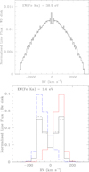 |
Fig. 7 Top: normalised individual fluorescent line profile of the Fe Κα line arising from the accretion disc around the WD in velocity bins of 50 km s−1. The primary X-ray source is located on the WD at a latitude of 30° (i.e. zs = 0.5 RWD). Bottom: Normalised individual fluorescent Fe Kα line contributed by the Be decretion disc illuminated by the WD at four orbital phases. The outer Be disc was assumed to follow the structure described by Rubio et al. (2025). The black histograms stand for the conjunction phases with the WD behind (solid line) or in front (dashed line). The blue and red histograms stand for the quadrature phases with the WD moving respectively towards us and away from us. |
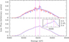 |
Fig. 8 Top: global line profile (i.e. combining the contributions from the WD’s accretion disc and the Be decretion disc and accounting for the full array of transitions) for our default non-magnetic WD model, at two opposite quadrature orbital phases. The profiles are shown as histograms with energy bins of 1 eV. Bottom: convolution of the global line profiles with an instrumental response function of 5 eV FWHM. The insert displays a zoom on the energy range 6480–6420 eV, to highlight the ~2.6 eV shift between the profiles at the extreme orbital phases. The magenta lines yield the theoretical energies of the centroids of the FeV Kαl and Kα2 subgroups. |
5.2 Accretion onto a magnetic white dwarf
In the accreting magnetic WD model, the primary X-ray emission is thought to arise in the shock-heated plasma of the post-shock accretion column (PSAC, see e.g. Hayashi & Ishida 2014). Immediately behind the shock, the plasma temperature follows from the pre-shock velocity, υpre-shock, via the Rankine-Hugoniot relations for strong shocks (e.g. Ezuka & Ishida 1999). Assuming a ballistic flow, from the Alfvén radius to the standoff shock, the post-shock temperature becomes
 (8)
(8)
where μ is the mean molecular weight and mH the mass of the hydrogen atom. Taking, for instance, RA = 20 RWD and hs = 0.5 RWD results in an expected plasma temperature of 27keV. This is well above the observational kT = 12.5 keV. As the shock-heated material settles towards the WD surface, its temperature rapidly decreases and its density increases. Hydro-dynamic models of the PSAC indicate that the regions close to the WD surface, which have the highest densities and thus the highest emission measure, display significantly lower plasma temperatures (see Fig. 2 of Hayashi & Ishida 2014). The temperature and density stratification of the PSAC yields an X-ray spectral energy distribution (Tsujimoto et al. 2018, 2023) that mimics that of conventional optically thin thermal plasma models of significantly lower kT (Rauw et al. 2022). For the simulations in this section, we kept the plasma temperature at kT = 12.5 keV, that is the mean value obtained from broadband X-ray spectral fitting of γ Cas (Rauw et al. 2022). This value should thus not be seen as the immediate post-shock temperature, but rather as an emission-measure-weighted average along the PSAC. In the same way, the hs parameter in our simulations should not be taken as the actual height of the standoff shock, but represents instead the height where most of the primary X-ray emission arises.
In this scenario, we must consider four reservoirs of fluorescent material. These are the WD photosphere, the truncated accretion disc, the pre-shock accretion flow and the circumstellar material of the Be star.
We first consider the contribution of the WD atmosphere. For this purpose, we used version 208 of the TLUSTY nLTE model atmosphere code (Hubeny & Lanz 2017a,b,c; Hubeny et al. 2021) to compute a WD model atmosphere with Teff = 60 000 K and log ɡ = 8.5. We considered three different situations. First, we assumed a hot DA WD with a nearly pure H atmosphere containing only traces of C (0.01 × solar) and Fe (0.4 × solar). As a second step, we considered a DO WD with a He abundance a hundred times that of hydrogen and the same traces of C and Fe (Nouh & Fouda 2007). For each case, we first built a pure H (or pure He + H) LTE model atmosphere. This model was then used as the starting point of an iterative process to compute a nLTE model. Finally, C and Fe were incorporated and the model was iterated to obtain a full nLTE solution (Hubeny & Lanz 2017c). In addition, we considered the moderately cool pure-H DA WD model (Teff = 10 000 K, log ɡ = 8.0) of Hubeny & Lanz (2017c).
For the two hot WD model atmospheres, the optical depth for photoelectric absorption of X-rays with energies above the Fe K edge reaches unity at higher Rosseland optical depths than in the case of the Be star (see Fig. 4). In the case of the DA WD, this occurs at τRoss ≃ 25, whereas it happens at τRoss ≃ 56 for the DO WD model. This difference with respect to the Be star is a consequence of the higher temperature and the low metal contents of the WD models. Both effects reduce the Rosseland opacity. According to our TLUSTY models, the dominant Fe ions at these optical depths are Fe V for the DA WD and Fe VI for the DO WD. Some studies of DA WDs indicate that metals might not be homogeneously distributed in the WD atmosphere, but could instead follow a stratification with nearly pure H or He atmospheres at the top (e.g. Rauch et al. 2013). Whilst our TLUSTY models were computed with rather low iron abundances and assuming a chemically homogeneous atmosphere without stratification, in the computation of the source function due to fluorescence, we assume a solar abundance. This assumption was introduced to account for stratification resulting in a higher Fe abundance at the τRoss where fluorescence occurs, and to ease comparison with other calculations in this paper which all assume solar Fe abundances.
We then used these WD model atmospheres in combination with our Feautrier method (Sect. 2.2 and Appendix A) to compute the WD’s photospheric contribution to the fluorescent line. We assume accretion near the WD’s magnetic poles which we consider, for simplicity, to coincide with the rotational poles. We further assume that the rotation and orbital axes are aligned and are seen under an angle i = 45° by the observer. We computed the EWs for different values of hs and considering all three WD atmosphere models (see top panel of Fig. 9). The hs parameter was varied between 0.005 RWD and 1.0 RWD in steps of 0.005 RWD for hs/RWD between 0.005 and 0.1, 0.01 RWD for hs/RWD between 0.1 and 0.2, 0.05 RWD for hs/RWD between 0.2 and 0.5, and 0.1 RWD for hs/RWD between 0.5 and 1.
For a primary X-ray source located at hs = 0.04 RWD above the WD’s pole, we obtain EWs of 3.68 eV and 4.90 eV respectively for the DA and DO WD models. This EW increases to 8.15 eV for the moderately cool DA WD. If we assume instead an extremely small hs = 0.001 RWD, then the hot and moderately cool DA WD atmospheres produce EWs of respectively 45.9 and 101.5 eV. These comparisons underline the strong dependence of the line strength on the unknown properties of the putative WD and of its accretion flow.
Finally, as one could expect given the WD’s rotational velocity, which is much lower than that of the Be star, the synthetic profiles of the individual components are extremely narrow (see Fig. 9). This conclusion is independent of the assumptions made for the WD atmospheric model and depends only on the adopted projected rotational velocity.
We can compare our results with those of van Teeseling et al. (1996) who considered the formation of the fluorescent Kα line via isotropical illumination of the WD atmosphere. In the absence of a strong temperature inversion, which occurs above a threshold value of the illuminating flux (see below), van Teeseling et al. (1996) predict an EW by reflection on the WD of about 57 eV for a WD with an effective temperature near 50 kK and considering a primary bremsstrahlung radiation with kT = 10 keV. Our EW values are much lower than those reported by van Teeseling et al. (1996). The reasons for this difference lie in their assumption of a fluorescent medium occupying a 2 π solid angle, as seen from the primary source, and undergoing isotropic illumination, that is with all fluorescent elements located at the same distance from the primary source. However, the actual geometry is that of a point source illuminating a sphere from the outside. As a result, only a limited cap with an extension in polar angle from 0 to arccos  of the WD surface will be illuminated. For hs = 0.04 RWD, this cap intercepts a solid angle of 0.725 × 2 π as seen from the primary source. Moreover, the majority of the illuminated parcels are farther away from the primary source than the parcel at the nadir point of the primary source and will thus receive a diluted flux. For hs = 0.04 RWD, the geometrical dilution produces a reduction of the EW by a factor 7. Finally, the EW obviously also depends on the viewing angle. Adopting i = 90° instead of 45° yields a 40% increase of the EW. Taken together, these effects can thus easily account for the lower EWs in our calculations compared to those of van Teeseling et al. (1996).
Additional uncertainties affect the level of the WD’s photospheric contribution. For instance, van Teeseling et al. (1996) drew attention to the fact that the optically thin layers at the top of an irradiated WD atmosphere can be subject to a temperature inversion if the primary flux exceeds 1016 erg cm−2 s−1. This leads to the occurrence of a range of ionisation stages resulting in fluorescent Kα line emission for ions up to Fe XXII. Because the energy of the lines increases for the highest ionisation stages, the energy domain between 6.4 and 6.6 keV gets populated with weaker fluorescent emissions. Hence the overall EW and the line width increase, and the centre of the whole fluorescent complex shifts towards higher energies. The maximum observed luminosities of γ Cas stars (Smith et al. 2016; Nazé & Motch 2018) yield an incident flux exceeding the threshold for temperature inversion for cases where hs < 0.16 RWD. Temperature inversion is currently not accounted for in our TLUSTY models which consider the X-rays as a perturbation of the atmosphere that does not alter its temperature and density structure.
The second most important contribution to the fluorescent line for the accreting magnetic WD scenario comes from the truncated accretion disc. Obviously, the WD Alfvén radius plays a key role here. Figure 10 illustrates the EW and the line width for individual fluorescent line components as a function of RA. The EW of this contribution is nearly insensitive to hs, but rapidly decreases from values near 27.6 eV, for RA = 2 RWD = 0.02 R⊙, to 8.8 eV, for RA = 8 RWD = 0.08 R⊙, and < 1 eV, for RA ≥ 80 RWD = 0.8 R⊙. The full width of the line is independent of hs and also displays a steep decrease with RA. This is expected as the truncation of the inner disc removes the material with the fastest orbital motion around the WD.
Finally, we address the contribution to the fluorescent line arising in the material of the magnetically channelled accretion flow. We assume here that the material flows along the magnetic field lines and the magnetic field can be described as dipolar. The field lines connect the inner boundary of the accretion disc, truncated at the Alfvén radius, with the magnetic pole of the WD. Assuming the relevant field line to be located in the (x, z) plane, we have x = RA sin3 θ, z = RA sin2 θ cos θ, and  sin2 θ. Following Hayashi et al. (2021), we assume that the material moves at the free fall velocity,
  , and that the accretion flow has a cross-section
  . Here S0 is the cross-section at the surface of the WD which is directly related to the accretion rate αacc by the expression
 (9)
(9)
Tsujimoto et al. (2018) applied the acrad model of Hayashi et al. (2018) for a magnetic accreting WD to the NuSTAR and Suzaku observations of γ Cas. In this model, the X-ray spectrum is computed as a function of WD mass by solving the plasma fluid equation along the magnetic field line and dealing with reprocessing of the X-rays that reflect off the WD surface6. In this way, Tsujimoto et al. (2018) inferred Ṁacc = 1.3 × 10⁻¹⁰ M⊙ yr−1 and log αacc = –0.61, where αacc is expressed in units g cm−2 s−1. This accretion rate is 6.5 times higher than the value found in the SPH calculations of Rast et al. (2025) and corresponds to a hydrogen number density of 1.8 × 1014 cm−3 at the Wd surface. To infer an optimistic value of the contribution of the accretion flow, we thus adopt the Tsujimoto et al. (2018) values. The number density decreases with distance from the WD as  (Hayashi et al. 2021), whilst the volume occupied by the flow increases as r4. We assume that accretion flows take place in both magnetic hemispheres.
Because of the high escape velocity of the WD, and because we assume that flows occur along field lines in both hemispheres, the contribution to the fluorescent line profile displays a broad profile with a double-peaked morphology (see Fig. 11). The peaks are quite narrow and their location depends on the aspect angle of the field lines with respect to the line of sight. The profiles are thus expected to change with the rotation phase of the WD’s magnetosphere (see Fig. 11). The EW of this contribution remains quite modest, however. For small Alfvén radii, the EW first increases with RA but quickly reaches a nearly constant value around 0.54 eV for RA ≥ 0.08 R⊙.
Finally, fluorescence from the illumination of the Be disc by the primary X-ray source located at the WD position is also included in our model (see Paper I). As for the non-magnetic WD case, this component yields rather low contribution of 1.4 eV to the EW.
Our ignorance of the properties of the putative WD and of the location of the accretion shock prevents us from computing all the ingredients of the magnetic WD model self-consistently. Nonetheless, we again combine all these ingredients to build a global line profile. For this purpose, we assume that the photospheric contribution has an EW of 50 eV, close to the observed EWs, and take a value of RA = 20 RWD. We then proceed as for the other scenarios to build the global Fe Kα line profile. The result is shown in Fig. 12. Whilst this specific model is not necessarily representative of the companion of γ Cas or any of its siblings, our calculations in this section nonetheless provide some important insight. First of all, the magnetic WD scenario can produce fluorescent lines with the strengths observed in γ Cas stars. The actual strength depends strongly on the properties of the WD atmosphere and to a lesser extent on its magnetic field strength. Our calculations suggest that cooler WDs are more efficient in producing fluorescent Fe Kα lines. However, given the expected youth of the WD in γ Cas which presumably formed as the outcome of a mass-exchange episode, the hot DA or DO WD models are probably more appropriate to describe the WDs associated with early-type Be stars. Second, synthetic line profiles are considerably narrower than those expected for a non-magnetic WD. The overall width is very similar to what we found for the magnetic star-disc interaction scenario. Finally, the centroids of the lines change with orbital phase as they are expected to follow the orbital motion of the WD, leading to a shift between quadrature phases of 2.6 eV which is measurable with Resolve and X-IFU.
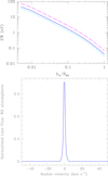 |
Fig. 9 Top: EW of the Fe Kα fluorescent line due to reflection on the WD surface as a function of the height of the accretion shock above the WD surface. The short-dashed cyan, solid blue, and long-dashed magenta lines correspond to the hot DA, the DO, and the moderately cool DA WD models, respectively. In all cases, an inclination of 45° was assumed. Bottom: synthetic profile for an individual component of the Fe Kα fluorescent line produced in the hot DA WD atmosphere for |

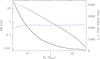 |
Fig. 10 Dependence of the EW and line width of individual fluorescent components from the truncated accretion disc and accretion flow on the WD Alfvén radius, RA. The grey-shaded area, with the corresponding vertical axis on the left, yields the total EW contributed by the accretion disc for values of hs ranging between 0.005 RWD and 1 RWD. The dashed blue curve indicates the EW contributed by the accretion flow. The solid black line yields the full width of the individual lines formed in the truncated accretion disc with the corresponding vertical axis on the right. |
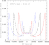 |
Fig. 11 Illustration of the expected individual line profiles for Fe Kα fluorescent lines arising from illumination of the material in the accretion flow. The Alfvén radius, RA, was taken to be 20 R* = 0.2 R⊙. The different lines correspond to different azimuthal rotation angles of the magnetosphere. The observer is located in the direction corresponding to the positive (x, z) plane and seeing the system under an inclination of i = 45°. The WD is located at the origin of the axes. The line colours correspond to orientations of the accretion flow located inside the positive (x, z) plane (continuous red line), the (y, z) plane (dashed black line), and the negative (x, z) plane (short dashed blue line). |
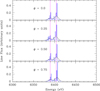 |
Fig. 12 Global Fe Kα lines for the case of an accreting magnetic WD assuming an EW of 50 eV for the component arising via reflection on the WD. We assume an Alfvén radius of 20 RWD = 0.2 R⊙. The blue histograms show the profiles with 1 eV energy bins, whereas the black lines show the results of a convolution with an instrumental response function of 5 eV FWHM. The magenta lines indicate the theoretical energies of the centroids of the Fe vi Kα1 and Kα2 subgroups (i.e. assuming Fe v target ions). We note the changes in energy of the line peaks, which amount to 2.6 eV between opposite quadrature phases. |
6 Conclusions
In this article, we investigated the fluorescent Fe Kα line profiles as they will be seen in high-resolution X-ray spectra of γ Cas stars according to the most-plausible scenarios: magnetic star-disc interaction or accretion by a WD companion. Our simulations indicate that the observable line profiles provide strong constraints on the origin of the hard primary X-ray emission. The most important constraints are summarised in Table 2.
For a non-magnetic accreting WD, the fluorescence mostly occurs in the WD accretion disc, close to the WD itself. Hence, the predicted global Fe Kα complex is very broad with a full width near 140 eV. In strong contrast with this situation, for the magnetic star-disc interaction and the magnetic accreting white dwarf cases, the full width of the Fe Ka complex is expected to be ~40 eV. This offers the first powerful diagnostic to distinguish the non-magnetic WD case from the other two scenarios.
Despite the very similar shapes of the overall line profiles, the magnetic star–disc interaction scheme and the magnetic WD scenario can also be distinguished thanks to the fluorescent line. Indeed, in the magnetic star–disc interaction, the inner decretion disc of the Be star provides the main reservoir of fluorescent material, which implies that the centroids of the Fe Kα transitions follow the orbital motion of the Be star. On the contrary, in the magnetic accreting WD configuration, the bulk of the fluorescence comes from the WD photosphere with some additional contributions from the WD accretion disc and the magnetically channelled accretion flow. In this case, the centroid of the line complex thus follows the motion of the WD, which is in antiphase with the motion of the Be star and has a significantly larger amplitude (around 2.6 eV for γ Cas).
Comparing upcoming XRISM/Resolve observations of γ Cas at some well-chosen orbital phases (orbital quadratures) with our synthetic line profiles will provide a major step forwards in the understanding of the mysterious X-ray emission of γ Cas stars. Provided the amplitudes of the expected RV excursions are larger than the instrumental precision and the observational data are of sufficient quality to determine precise line widths and centroids, XRISM observations at several well-selected orbital phases should enable us to differentiate between the competing scenarios. Whilst XRISM observations will be restricted to the X-ray-brightest objects of the γ Cas category, Athena/X-IFU should be able to collect such data for a larger number of γ Cas stars, with different stellar and binary properties. This will allow us to sample the γ Cas population at large and enable a better understanding of the evolutionary status of these systems.
Summary of expected fluorescent Fe Kα line properties.
Acknowledgements
This study was partially supported by the BELgian federal Science Policy Office (BELSPO) and the European Space Agency through the PRODEX HERMeS grant. ADS and CDS were used during this research. My deepest gratitude goes to Drs Yaël Nazé, Myron Smith, Christian Motch, and Masahiro Tsujimoto for discussion, and to the referee for remarks that helped me improve this work.
Appendix A Fluorescence in the stellar atmosphere
In a plane-parallel atmosphere, we have
 (A.1)
(A.1)
with IE (z, μ, Ε) the specific intensity per unit photon energy at energy E at coordinate z and propagating in the direction μ, p(z) is the gas density, η(z, Ε) and χ(z, Ε) are respectively the emissivity and opacity at energy E and depth z.
Using the Rosseland optical depth dτRoss = –κROSS ρ dz, Eq. (A.1) becomes
 (A.2)
(A.2)
where  , and S (τROSS, E) is the source function. Restricting μ to positive values (0 ≤ μ ≤ 1), we can split IE into two regimes (outwards-propagating and inwards-propagating):
 (A.3)
(A.3)
 (A.4)
(A.4)
We then define
 (A.5)
(A.5)
 (A.6)
(A.6)
Hence, Eq. (A.2) leads to
 (A.7)
(A.7)
 (A.8)
(A.8)
which finally yields
 (A.9)
(A.9)
Equation (A.9) is solved with the boundary conditions
 (A.10)
 (A.11)
where ΙX,E is the illuminating specific intensity per unit photon energy which is non-zero only for the value of μ corresponding to the angle of illumination by the external X-ray source. We follow García et al. (2013) in expressing this quantity as
 (A.12)
where F(E) is the flux at energy E illuminating the photosphere.
The source function has two contributions:
• electron scattering which we treat as in García & Kallman (2010) with
 (A.13)
where αKN is the Klein-Nishina cross-section,  ,
,  and
and  is the mean intensity per unit photon energy at an energy E′.
• fluorescent emission which we express as
 (A.14)
where σK–shell(E′) is the K-shell photo-ionisation cross-section computed according to Verner & Yakovlev (1995), Ethres is the threshold energy for K-shell ionisation, zFe is the abundance of iron with respect to hydrogen (Asplund et al. 2009), xion is the relative abundance of a specific Fe ion, and ωion+1 the associated Kα fluorescent yield (Kallman et al. 2004).
The above set of equations is solved in an iterative way. The iterations are stopped when the χ2 evaluated from the relative differences of JE in consecutive iterations drop below 10−5. Convergence depends on the value of μin, but is usually achieved within less than ten iterations. The outwards propagating specific intensity is directly proportional to the intensity of the incoming X-ray emission and is not sensitive to the initial approximation of  (either taken to be zero or equal to the intensity of the incoming X-rays multiplied by exp (–τROSS)).
References
- Asplund, M., Grevesse, N., Sauval, A. J., & Scott, P. 2009, ARA&A, 47, 481 [NASA ADS] [CrossRef] [Google Scholar]
- Byckling, K., Mukai, K., Thorstensen, J. R., & Osborne, J. P. 2010, MNRAS, 408, 2298 [NASA ADS] [CrossRef] [Google Scholar]
- Cantiello, M., & Braithwaite, J. 2011, A&A, 534, A140 [NASA ADS] [CrossRef] [EDP Sciences] [Google Scholar]
- Eze, R. N. C. 2015, New A, 37, 35 [Google Scholar]
- Ezuka, H., & Ishida, M. 1999, ApJS, 120, 277 [NASA ADS] [CrossRef] [Google Scholar]
- García, J., & Kallman, T. R. 2010, ApJ, 718, 695 [CrossRef] [Google Scholar]
- García, J., Dauser, T., Reynolds, C. S., et al. 2013, ApJ, 768, 146 [Google Scholar]
- Gies, D. R., Wang, L., & Klement, R. 2023, ApJ, 942, L6 [NASA ADS] [CrossRef] [Google Scholar]
- Hailey, C. J., Mori, K., Perez, K., et al. 2016, ApJ, 826, 160 [NASA ADS] [CrossRef] [Google Scholar]
- Hamaguchi, K., Oskinova, L., Russell, C. M. P., et al. 2016, ApJ, 832, 140 [NASA ADS] [CrossRef] [Google Scholar]
- Hayashi, T., & Ishida, M. 2014, MNRAS, 438, 2267 [Google Scholar]
- Hayashi, T., Kitaguchi, T., & Ishida, M. 2018, MNRAS, 474, 1810 [Google Scholar]
- Hayashi, T., Kitaguchi, T., & Ishida, M. 2021, MNRAS, 504, 3651 [NASA ADS] [CrossRef] [Google Scholar]
- Hubeny, I., & Lanz, T. 2017a, arXiv e-prints [arXiv:1706.01859] [Google Scholar]
- Hubeny, I., & Lanz, T. 2017b, arXiv e-prints [arXiv:1706.01935] [Google Scholar]
- Hubeny, I., & Lanz, T. 2017c, arXiv e-prints [arXiv:1706.01937] [Google Scholar]
- Hubeny, I., Allende Prieto, C., Osorio, Y., & Lanz, T. 2021, arXiv e-prints [arXiv:2104.02829] [Google Scholar]
- Huenemoerder, D. P., Pradhan, P., Canizares, C. R., et al. 2024, ApJ, 966, L23 [Google Scholar]
- Hummel, W., & Vrancken, M. 2000, A&A, 359, 1075 [NASA ADS] [Google Scholar]
- Ishisaki, Y., Kelley, R. L., Awaki, H., et al. 2022, SPIE Conf. Ser., 12181, 121811S [NASA ADS] [Google Scholar]
- Jernigan, J. G. 1976, IAU Circ., 2900, 2 [NASA ADS] [Google Scholar]
- Kallman, T. R., Palmeri, P., Bautista, M. A., Mendoza, C., & Krolik, J. H. 2004, ApJS, 155, 675 [Google Scholar]
- Kennea, J. A., Coe, M. J., Evans, P. A., et al. 2021, MNRAS, 508, 781 [NASA ADS] [CrossRef] [Google Scholar]
- Kurfürst, P., Feldmeier, A., & Krticka, J. 2014, A&A, 569, A23 [NASA ADS] [CrossRef] [EDP Sciences] [Google Scholar]
- Langer, N., Baade, D., Bodensteiner, J., et al. 2020, A&A, 633, A40 [NASA ADS] [CrossRef] [EDP Sciences] [Google Scholar]
- Lanz, T., & Hubeny, I. 2007, ApJS, 169, 83 [CrossRef] [Google Scholar]
- Lopes de Oliveira, R., & Mukai, K. 2019, ApJ, 880, 128 [NASA ADS] [CrossRef] [Google Scholar]
- Lopes de Oliveira, R., Motch, C., Haberl, F., Negueruela, I., & Janot-Pacheco, E. 2006, A&A, 454, 265 [NASA ADS] [CrossRef] [EDP Sciences] [Google Scholar]
- Martin, R. G., Lubow, S. H., Armitage, P. J., & Price, D. J. 2024, MNRAS, 530, 4148 [Google Scholar]
- Mason, K. O., White, N. E., & Sanford, P. W. 1976, Nature, 260, 690 [Google Scholar]
- Motch, C., Lopes de Oliveira, R., & Smith, M. A. 2015, ApJ, 806, 177 [NASA ADS] [CrossRef] [Google Scholar]
- Mukai, K. 2017, PASP, 129, 062001 [Google Scholar]
- Murakami, T., Koyama, K., Inoue, H., & Agrawal, P. C. 1986, ApJ, 310, L31 [NASA ADS] [CrossRef] [Google Scholar]
- Nazé, Y. 2025, Galaxies, 13, 8 [Google Scholar]
- Nazé, Y., & Motch, C. 2018, A&A, 619, A148 [NASA ADS] [CrossRef] [EDP Sciences] [Google Scholar]
- Nazé, Y., & Robrade, J. 2023, MNRAS, 525, 4186 [CrossRef] [Google Scholar]
- Nazé, Y., Motch, C., Rauw, G., et al. 2020, MNRAS, 493, 2511 [CrossRef] [Google Scholar]
- Nazé, Y., Rauw, G., Czesla, S., Smith, M. A., & Robrade, J. 2022a, MNRAS, 510, 2286 [CrossRef] [Google Scholar]
- Nazé, Y., Rauw, G., Smith, M. A., & Motch, C. 2022b, MNRAS, 516, 3366 [CrossRef] [Google Scholar]
- Nouh, M. I., & Fouda, D. A. 2007, Contrib. Astron. Observ. Skalnate Pleso, 37, 189 [Google Scholar]
- Okazaki, A. T., & Negueruela, I. 2001, A&A, 377, 161 [NASA ADS] [CrossRef] [EDP Sciences] [Google Scholar]
- Okazaki, A. T., Bate, M. R., Ogilvie, G. I., & Pringle, J. E. 2002, MNRAS, 337, 967 [NASA ADS] [CrossRef] [Google Scholar]
- Page, K. L., & Shaw, A. W. 2022, in Handbook of X-ray and Gamma-ray Astrophysics, eds. C. Bambi, & A. Sangangelo, 107 [Google Scholar]
- Palmeri, P., Mendoza, C., Kallman, T. R., Bautista, M. A., & Meléndez, M. 2003, A&A, 410, 359 [NASA ADS] [CrossRef] [EDP Sciences] [Google Scholar]
- Pandel, D., & Córdova, F. A. 2005, ApJ, 620, 416 [NASA ADS] [CrossRef] [Google Scholar]
- Panoglou, D., Carciofi, A. C., Vieira, R. G., et al. 2016, MNRAS, 461, 2616 [Google Scholar]
- Peille, P., Barret, D., Cucchetti, E., et al. 2025, Exp. Astron., 59, 18 [Google Scholar]
- Postnov, K., Oskinova, L., & Torrejón, J. M. 2017, MNRAS, 465, L119 [Google Scholar]
- Ramsay, G., & Cropper, M. 2007, MNRAS, 379, 1209 [NASA ADS] [CrossRef] [Google Scholar]
- Ramsay, G., Cropper, M., Córdova, F., et al. 2001, MNRAS, 326, L27 [Google Scholar]
- Rast, R., Nazé, Y., Labadie-Bartz, J., et al. 2025, Ap&SS, 370, 108 [Google Scholar]
- Rauch, T., Werner, K., Bohlin, R., & Kruk, J. W. 2013, A&A, 560, A106 [NASA ADS] [CrossRef] [EDP Sciences] [Google Scholar]
- Rauw, G. 2024, A&A, 682, A179 [NASA ADS] [CrossRef] [EDP Sciences] [Google Scholar]
- Rauw, G., Nazé, Y., Motch, C., et al. 2022, A&A, 664, A184 [NASA ADS] [CrossRef] [EDP Sciences] [Google Scholar]
- Rivinius, T., Carciofi, A. C., & Martayan, C. 2013, A&A Rev., 21, 69 [NASA ADS] [CrossRef] [Google Scholar]
- Robinson, R. D., & Smith, M. A. 2000, ApJ, 540, 474 [NASA ADS] [CrossRef] [Google Scholar]
- Rubio, A. C., Carciofi, A. C., Bjorkman, J. E., et al. 2025, A&A, 698, A309 [NASA ADS] [CrossRef] [EDP Sciences] [Google Scholar]
- Shao, Y., & Li, X.-D. 2014, ApJ, 796, 37 [Google Scholar]
- Smith, M. A. 2019, PASP, 131, 044201 [NASA ADS] [CrossRef] [Google Scholar]
- Smith, M. A., & Balona, L. 2006, ApJ, 640, 491 [NASA ADS] [CrossRef] [Google Scholar]
- Smith, M. A., & Robinson, R. D. 1999, ApJ, 517, 866 [NASA ADS] [CrossRef] [Google Scholar]
- Smith, M. A., Robinson, R. D., & Corbet, R. H. D. 1998, ApJ, 503, 877 [NASA ADS] [CrossRef] [Google Scholar]
- Smith, R. K., Brickhouse, N. S., Liedahl, D. A., & Raymond, J. C. 2001, ApJ, 556, L91 [Google Scholar]
- Smith, M. A., Lopes de Oliveira, R., & Motch, C. 2016, Adv. Space Res., 58, 782 [Google Scholar]
- Smith, M. A., Lopes de Oliveira, R., & Motch, C. 2017, MNRAS, 469, 1502 [NASA ADS] [CrossRef] [Google Scholar]
- Toalá, J. A., Oskinova, L. M., & Vasquez-Torres, D. A. 2025, MNRAS, 542, 876 [Google Scholar]
- Tsujimoto, M., Hayashi, T., Morihana, K., & Moritani, Y. 2023, PASJ, 75, 177 [NASA ADS] [CrossRef] [Google Scholar]
- Tsujimoto, M., Morihana, K., Hayashi, T., & Kitaguchi, T. 2018, PASJ, 70, 109 [NASA ADS] [Google Scholar]
- van Teeseling, A., Kaastra, J. S., & Heise, J. 1996, A&A, 312, 186 [NASA ADS] [Google Scholar]
- Verner, D. A., & Yakovlev, D. G. 1995, A&AS, 109, 125 [NASA ADS] [Google Scholar]
- White, N. E., Swank, J. H., Holt, S. S., & Parmar, A. N. 1982, ApJ, 263, 277 [NASA ADS] [CrossRef] [Google Scholar]
- Xu, X.-j., Wang, Q. D., & Li, X.-D. 2016, ApJ, 818, 136 [NASA ADS] [CrossRef] [Google Scholar]
- Yamaguchi, H., Eriksen, K. A., Badenes, C., et al. 2014, ApJ, 780, 136 [Google Scholar]
Langer et al. (2020) proposed a collision between the wind of a hot stripped star and the Be disc as the origin of the hard X-ray emission. However, this scenario was found to be in contradiction with observations (Nazé et al. 2022b).
The fluorescent Fe Κα line observed in the XMM-Newton and Chandra spectra of γ Cas has an EW in the range between 34 and 59 eV (Rauw et al. 2022).
Reabsorption is restricted to the inner disc. The contribution of the spiral arms is negligible.
If we increase the density by a factor of four with respect to our baseline value, the EW actually decreases to 33.3 eV because the disc becomes optically thick over a wider range in radii.
That is the Keplerian velocity on a circular orbit of radius equal to the stellar radius.
The WD surface is approximated as a solid in this model.
All Tables
All Figures
|
Fig. 1 Upper box: schematic pole-on view of the Be star (blue dot), its decretion disc and spiral extensions (sky blue), the WD companion, and its truncated accretion disc (magenta). The dark blue contour shows the Roche lobe of the system. The boxes at the bottom provide zooms on vertical cuts through the inner part of the Be decretion disc (left) and the surroundings of the WD (shown by the violet dot) with its magnetically truncated accretion disc (right). The red crosses correspond to the emitting regions of the primary X-rays. The left box illustrates the case of the magnetic star-disc interaction with magnetic field lines that connect the star and the disc. The right box corresponds to an accreting magnetic WD scenario where a magnetically channelled flow connects the truncated accretion disc to the magnetic poles of the WD. |
| In the text | |
|
Fig. 2 Normalised individual Fe Κα line profile contributed by the Be decretion disc assuming an extended source represented by two rings of hot plasma of radius 1.5 R* and located 0.5 R* above or below the Be decretion disc. The line profile is binned into velocity bins of 50 km s−1 and is normalised by dividing by the total flux over the entire line profile. The spectral energy distribution of the illuminating source is an optically thin thermal plasma model with kT = 12.5 keV. The red histogram corresponds to an axisymmetric disc truncated at r = 176 R⊙. The blue histogram yields the results for a disc with spiral extensions as described in the text and computed out to a = 375 R⊙. The normalised profiles are displayed in velocity bins of 50 km s−1. |
| In the text | |
|
Fig. 3 Top: EW of the fluorescent Fe Κα line contributed by the Be decretion disc in the star-disc interaction scenario as a function of Rs for different values of Zs. Bottom: EW contours for the same scenario as a function of Rs and Zs. The primary source is modelled as a uniform axisymmetric ring of radius Rs from the polar axis of the Be star and of altitude Zs above the equatorial plane of the Be star. The hatched area in the bottom part corresponds to the scale height of the Be decretion disc. |
| In the text | |
|
Fig. 4 Rosseland optical depth inside the photosphere where the optical depth for photoelectric absorption of X-rays reaches unity. The continuous red line illustrates the results for the Teff = 25 000 K, log ɡ = 3.75 TLUSTY model adopted for the Be star. The short-dashed cyan line and the long-dashed blue line correspond respectively to DA and DO WD models with Teff = 60 000 K and log ɡ = 8.5. |
| In the text | |
|
Fig. 5 Individual Fe Kα line profile contributed by the Be photosphere. The illuminating source is an extended ring-like source located at Rs = 1.5 R* and Zs = 0.5 R*. The spectral energy distribution of the illuminating source is an optically thin thermal plasma model with kT = 12.5 keV. |
| In the text | |
|
Fig. 6 Top: global line profile (i.e. combining the Be-disc and photo-spheric contributions and accounting for the full array of transitions) for our default magnetic interaction model, at two opposite quadrature orbital phases. The profiles are shown as histograms binned in energy bins of 1 eV. Bottom: convolution of the global line profiles with an instrumental response function of 5 eV FWHM. The magenta lines yield the theoretical energies of the centroids of the Fe V Kα1 and Kα2 subgroups (Palmeri et al. 2003) assuming Fe IV target ions. |
| In the text | |
|
Fig. 7 Top: normalised individual fluorescent line profile of the Fe Κα line arising from the accretion disc around the WD in velocity bins of 50 km s−1. The primary X-ray source is located on the WD at a latitude of 30° (i.e. zs = 0.5 RWD). Bottom: Normalised individual fluorescent Fe Kα line contributed by the Be decretion disc illuminated by the WD at four orbital phases. The outer Be disc was assumed to follow the structure described by Rubio et al. (2025). The black histograms stand for the conjunction phases with the WD behind (solid line) or in front (dashed line). The blue and red histograms stand for the quadrature phases with the WD moving respectively towards us and away from us. |
| In the text | |
|
Fig. 8 Top: global line profile (i.e. combining the contributions from the WD’s accretion disc and the Be decretion disc and accounting for the full array of transitions) for our default non-magnetic WD model, at two opposite quadrature orbital phases. The profiles are shown as histograms with energy bins of 1 eV. Bottom: convolution of the global line profiles with an instrumental response function of 5 eV FWHM. The insert displays a zoom on the energy range 6480–6420 eV, to highlight the ~2.6 eV shift between the profiles at the extreme orbital phases. The magenta lines yield the theoretical energies of the centroids of the FeV Kαl and Kα2 subgroups. |
| In the text | |
|
Fig. 9 Top: EW of the Fe Kα fluorescent line due to reflection on the WD surface as a function of the height of the accretion shock above the WD surface. The short-dashed cyan, solid blue, and long-dashed magenta lines correspond to the hot DA, the DO, and the moderately cool DA WD models, respectively. In all cases, an inclination of 45° was assumed. Bottom: synthetic profile for an individual component of the Fe Kα fluorescent line produced in the hot DA WD atmosphere for |
| In the text | |
|
Fig. 10 Dependence of the EW and line width of individual fluorescent components from the truncated accretion disc and accretion flow on the WD Alfvén radius, RA. The grey-shaded area, with the corresponding vertical axis on the left, yields the total EW contributed by the accretion disc for values of hs ranging between 0.005 RWD and 1 RWD. The dashed blue curve indicates the EW contributed by the accretion flow. The solid black line yields the full width of the individual lines formed in the truncated accretion disc with the corresponding vertical axis on the right. |
| In the text | |
|
Fig. 11 Illustration of the expected individual line profiles for Fe Kα fluorescent lines arising from illumination of the material in the accretion flow. The Alfvén radius, RA, was taken to be 20 R* = 0.2 R⊙. The different lines correspond to different azimuthal rotation angles of the magnetosphere. The observer is located in the direction corresponding to the positive (x, z) plane and seeing the system under an inclination of i = 45°. The WD is located at the origin of the axes. The line colours correspond to orientations of the accretion flow located inside the positive (x, z) plane (continuous red line), the (y, z) plane (dashed black line), and the negative (x, z) plane (short dashed blue line). |
| In the text | |
|
Fig. 12 Global Fe Kα lines for the case of an accreting magnetic WD assuming an EW of 50 eV for the component arising via reflection on the WD. We assume an Alfvén radius of 20 RWD = 0.2 R⊙. The blue histograms show the profiles with 1 eV energy bins, whereas the black lines show the results of a convolution with an instrumental response function of 5 eV FWHM. The magenta lines indicate the theoretical energies of the centroids of the Fe vi Kα1 and Kα2 subgroups (i.e. assuming Fe v target ions). We note the changes in energy of the line peaks, which amount to 2.6 eV between opposite quadrature phases. |
| In the text | |
Current usage metrics show cumulative count of Article Views (full-text article views including HTML views, PDF and ePub downloads, according to the available data) and Abstracts Views on Vision4Press platform.
Data correspond to usage on the plateform after 2015. The current usage metrics is available 48-96 hours after online publication and is updated daily on week days.
Initial download of the metrics may take a while.