| Issue |
A&A
Volume 703, November 2025
|
|
|---|---|---|
| Article Number | L6 | |
| Number of page(s) | 9 | |
| Section | Letters to the Editor | |
| DOI | https://doi.org/10.1051/0004-6361/202556473 | |
| Published online | 05 November 2025 | |
Letter to the Editor
The variability angular diameter distance and the intrinsic brightness temperature of active galactic nuclei
1
University of Science and Technology, 217 Gajeong-ro, Yuseong-gu, Daejeon 34113, Republic of Korea
2
Korea Astronomy and Space Science Institute, 776 Daedeok-daero, Yuseong-gu, Daejeon 34055, Republic of Korea
3
Department of Physics and Astronomy, Sejong University, 209 Neungdong-ro, Gwangjin-gu, Seoul, Republic of Korea
⋆ Corresponding authors: This email address is being protected from spambots. You need JavaScript enabled to view it.
; This email address is being protected from spambots. You need JavaScript enabled to view it.
Received:
17
July
2025
Accepted:
14
October
2025
Abstract
Context. It has recently been suggested that angular diameter distances derived from comparing the variability timescales of blazars to angular size measurements with very long baseline interferometry (VLBI) may provide an alternative method to study the cosmological evolution of the Universe. Once the intrinsic brightness temperature (Tint) is known, the angular diameter distance may be found without knowledge of the relativistic Doppler factor, opening up the possibility of a single rung distance measurement method from low (zcos ≪ 1) to high (zcos > 4) redshifts. Previous studies have found Tint ≈ 1010–1011 K, with a potential frequency dependence.
Aims. We aim to verify whether the variability-based estimates of the intrinsic brightness temperature of multiple active galactic nuclei (AGNs) converges to a common value. We also investigate whether the intrinsic brightness temperature changes as a function of frequency.
Methods. We estimated the Tint of AGNs based on the flux variability of the radio cores of their jets. We utilized radio core light curves and size measurements of 75 sources at 15 GHz and of 37 sources at 43 GHz. We also derived Tint from a population study of the brightness temperatures of VLBI cores using VLBI survey data of more than 100 sources at 24, 43, and 86 GHz.
Results. Radio core variability-based estimates of Tint constrain upper limits of log10Tint [K] < 11.56 at 15 GHz and log10Tint [K] < 11.65 at 43 GHz under a certain set of geometric assumptions. The population analysis suggests lower limits of log10Tint [K] > 9.7, 9.1, and 9.3 respectively at 24, 43, and 86 GHz. Even with monthly observations, variability-based estimates of Tint appear to be cadence-limited.
Conclusions. Methods used to constrain Tint are more uncertain than previously thought. However, with improved datasets, the estimates should converge.
Key words: galaxies: active / galaxies: jets
© The Authors 2025
 Open Access article, published by EDP Sciences, under the terms of the Creative Commons Attribution License (https://creativecommons.org/licenses/by/4.0), which permits unrestricted use, distribution, and reproduction in any medium, provided the original work is properly cited.
This article is published in open access under the Subscribe to Open model. This email address is being protected from spambots. You need JavaScript enabled to view it. to support open access publication.
1. Introduction
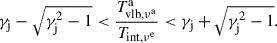
With the continued presence of the Hubble tension (Planck Collaboration VI 2020; Riess et al. 2022) and hints of evolving dark energy (Adame et al. 2025), it is of ever-growing importance to cross evaluate the known cosmological parameters with multiple independent methods. One such method uses the ratio of the observed angular size and the causality-limited size to determine the angular diameter distance to a variable source (Wiik & Valtaoja 2001; Hodgson et al. 2020) . The idea stems from the assumption that the variability timescale, Δt, of a source connects to the physical size of the emission region as
 (1)
(1)
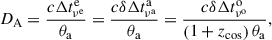
where a is the radial size of the source (if f = 0.5, cΔt corresponds to the diameter), c is the speed of light, and f is some correction factor equating the causality size (cΔt) to the physical linear size. A correlation between a (or the angular radial size θa) and Δt has been found in active galactic nuclei (AGNs) (see e.g., Hsu et al. 2023), supporting our assumptions. From the definition of the angular diameter distance, we then have (Hodgson et al. 2020)
![Mathematical equation: $$ \begin{aligned} D_{\rm A} = \frac{a}{\theta _{\rm a}} = \frac{fc\delta \Delta t^\mathrm{o}_{\nu ^\mathrm{o}}}{\left[1+z_{\rm cos}\right]\theta _{\rm a}}, \end{aligned} $$](/articles/aa/full_html/2025/11/aa56473-25/aa56473-25-eq2.gif) (2)
(2)
where we have taken (here, as well as in the remainder of the text) f = 1, Δtνoo as the variability timescale (Δto) measured in the observer frame, ℱo (denoted with the superscript “o”), at frequency νo; zcos is the cosmological redshift of the source; and θa is the angular size.
The calculation of DA using Equation (2) requires knowledge of the Doppler factor, δ, in order to correct for potential unknown special relativistic effects. Hodgson et al. (2023) assumed a common maximum intrinsic brightness temperature (Tint) to remove an explicit dependence on δ. It was found that
 (3)
(3)
where νe = νo[1+zcos]/δ is the frequency of the observed photon in the emission frame (denoted with the superscript “e”). The very long baseline interferometry (VLBI) measured angular size θvlb = BθFWHM is the full width at half maximum (FWHM) of the fit Gaussian component (θFWHM) multiplied by some correction factor, B, that accounts for the source geometry. Typically, Gaussians are fit to visibilities to determine component angular sizes. However, a Gaussian is not a realistic approximation of the true source geometry. In principle, with high quality observations, the true source geometry may be measured (Lobanov 2015).
The assumption of a common value of Tint over different sources and frequencies may not be correct. Previous studies (e.g., Liodakis et al. 2018; Homan et al. 2006, 2021; Lee 2013, 2014; Lobanov et al. 2000; Nair et al. 2019) using various methods have found values of Tint of ∼1010–1011 K. Lee (2014) assumed a population model of AGNs to suggest a possible frequency dependence of the value of Tint, peaking at νo ∼ 10 GHz. Such a frequency dependence, if left unaccounted for, will introduce a redshift-dependent bias into the cosmological measurements using the Tint assumption. By switching Tint, νe and DA in Equation (3), we can estimate the Tint for an individual source with constrained values of Δt, Sν, θvlb, and zcos and an assumed cosmology. The purpose of this paper is to a) utilize a refined version of Equation (3) to verify whether the Tint calculated for multiple sources does indeed converge at a certain value and b) with additional Tvlb versus apparent speed (βapp) analysis at 24, 43, and 86 GHz, investigate whether there is indeed a frequency dependence of Tint.
2. Estimating the intrinsic brightness temperature
The intrinsic brightness temperature, Tint, of the emission region is difficult to obtain, as the observed brightness temperature is affected by δ. While δ may be estimated under various assumptions (e.g., Jorstad et al. 2017; Hovatta et al. 2009; Liodakis et al. 2017; Ghisellini et al. 1993; Readhead 1994; Guijosa & Daly 1996), it is of interest to derive Tint independently of δ. We utilized the following two methods to do so.
2.1. Variability-based estimate
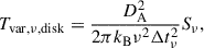
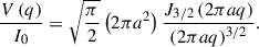
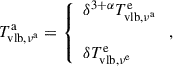
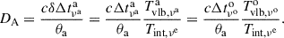
The (causality) constrained physical extent of the emission region and the definition of the angular diameter distance DA may be used to obtain Equation (2). Parameters defined in the host-galaxy frame, ℱa, are denoted with the superscript “a” (i.e., νo = νa/[1+zcos] = δνe/[1+zcos]). Following Hodgson et al. (2023), we substituted δ = Tvlb, νaa/Tint, νe to find
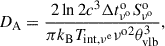
![Mathematical equation: $$ \begin{aligned} D_{\rm A} =\frac{c\Delta t^\mathrm{o}_{\nu ^\mathrm{o}}}{\left[1+z_{\rm cos}\right]\theta _{\rm a}}\frac{T^\mathrm{a}_{\rm vlb,\nu ^\mathrm{a}}}{T_{\rm int,\nu ^\mathrm{e}}} =\frac{c\Delta t^\mathrm{o}_{\nu ^\mathrm{o}}}{\theta _{\rm a}}\frac{T^\mathrm{o}_{\rm vlb,\nu ^\mathrm{o}}}{T_{\rm int,\nu ^\mathrm{e}}}, \end{aligned} $$](/articles/aa/full_html/2025/11/aa56473-25/aa56473-25-eq4.gif) (4)
(4)
where Tint, ν is the intrinsic brightness temperature of the source and Tvlb, ν is the VLBI-measured brightness temperature.
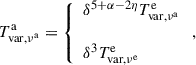
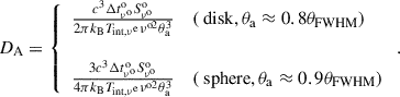
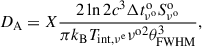
Proceeding further, we assumed either a uniform circular disk or an optically thin spherical geometry as more realistic models for the emission region. Taking θFWHM as the angular FWHM of the model-fit Gaussian component, the total radial angular size of a uniform disk is θa ≈ 0.8θFWHM and that of a sphere is θa ≈ 0.9θFWHM (e.g., Pearson 1995). Based on these approximations, we rewrote Equation (3) to solve for Tint, νe as
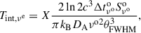 (5)
(5)
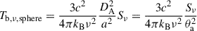
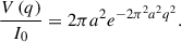
where X equals 1 for a Gaussian, ≈0.70 for a disk, and ≈0.74 for a sphere (see Appendix A for details). For a source with a known characteristic variability timescale, flux density, size, and (angular diameter) distance, we can evaluate the intrinsic brightness temperature, Tint, νe, in the emission frame, ℱe, without prior knowledge of the Doppler factor, δ. It should be noted that this is equivalent to estimating Tint, ν from Tvlb, ν and the variability brightness temperature (Tvar, ν) as  . It is assumed that Tvlb, ν and Tvar, ν are calculated for the same emission region geometry and that the same flux density value, Sνoo, is used. In Hodgson et al. (2023), assuming a Gaussian geometry, Tint, νe was found to be of ∼4 × 10¹¹ K. We find that Tint, νe estimated with Equation (5) is ∼4 × 10¹⁰ K (see Appendix C). We emphasize that inconsistent use of geometric assumptions can lead to differences of approximately an order of magnitude in the derived quantities.
2.2. Population study with Tvlb, ν and βapp
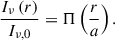
A different method of estimating Tint utilizes the distribution of the apparent speeds, βapp, of the jet with respect to Tvlb, νaa (Homan et al. 2006, 2021). From special relativity, we have δ = [γj(1−βj cos θj)]−1 and βapp = βj sin θj/(1−βj cos θj). Here,  is the bulk Lorentz factor of the jet, and θj is the viewing angle (i.e., the angle between the jet axis and the line of sight). For a given γj, we can estimate βapp as
![Mathematical equation: $$ \begin{aligned} \beta _{\rm app} =\left[\frac{2\gamma _{\rm j}T_{\rm vlb,\nu ^\mathrm{a}}^\mathrm{a}}{T_{\rm int,\nu ^\mathrm{e}}}-\left(\frac{T_{\rm vlb,\nu ^\mathrm{a}}^\mathrm{a}}{T_{\rm int,\nu ^\mathrm{e}}}\right)^2-1\right]^{\frac{1}{2}} . \end{aligned} $$](/articles/aa/full_html/2025/11/aa56473-25/aa56473-25-eq8.gif) (6)
(6)
For a source with given Tint, νe and γj, the observed Tvlb, νaa and βapp varies due to θj. The maximum observable apparent speed (βmax) of
![Mathematical equation: $$ \begin{aligned} \beta _{\rm max}=\left[\left(\frac{T_{\rm vlb,\nu ^\mathrm{a}}^\mathrm{a}}{T_{\rm int,\nu ^\mathrm{e}}}\right)^2-1\right]^{\frac{1}{2}}, T_{\rm int,\nu ^\mathrm{e}}\le T_{\rm vlb,\nu ^\mathrm{a}}^\mathrm{a} \end{aligned} $$](/articles/aa/full_html/2025/11/aa56473-25/aa56473-25-eq9.gif) (7)
(7)
is obtained when the jet is viewed at the critical angle θj = θc ≡ arccosβj. For a flux-limited sample of sources with a common Tint, νe, approximately 75% of the sources are expected to have viewing angles of θj < θc (Homan et al. 2006; Lee 2013). This manifests as 75% of sources lying below the βmax line in the βapp versus Tvlb, νaa parameter space. Under these assumptions, all βapp measurements should lie under the envelope provided by the maximum observed βapp (solid line in Figure B.2). Therefore, we may constrain the value of Tint, νe using a flux-limited sample of AGNs with known βapp and Tvlb, νaa (Homan et al. 2006, 2021; Lee 2013, 2014).
2.3. Data analysis
For the variability-based analysis (Section 2.1), we applied Equation (5) to the archival Very Long Baseline Array (VLBA) data from the MOJAVE program1 at 15 GHz (Lister et al. 2018) and the Boston University VLBA-BU-BLAZAR 43 GHz monitoring program2 (Jorstad et al. 2017; Weaver et al. 2022). We collected multi-epoch core fluxes and sizes for multiple sources as a result of model-fitting multiple Gaussian components to the observed visibilities. At 15 GHz, we utilized the tabulated data published in Homan et al. (2021). At 43 GHz, we combined the data from 2007 June to 2012 December in Jorstad et al. (2017) and from 2013 January to 2018 December in Weaver et al. (2022). For each source, we evaluated the variability timescale for each pair of consecutive measurements as
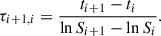
We used τi + 1, i, along with the flux density and size measurements of the epoch with the larger flux density to calculate Tint for each measurement pair. When doing so, we only kept values for which both θFWHM, i + 1 and θFWHM, i were marked as resolved in the original publications, and only if τi + 1, i > 0 (i.e., the flux density is rising between consecutive measurements). From the constraint on τi + 1, i, we ultimately utilized Si + 1 and θi + 1 for our flux density and size measurements. The two-point estimate of τi + 1, i relies on significant flux variability measurements with a cadence comparable to, or better than, the variability timescale of the flare in question. Estimates of τi + 1, i may be biased toward larger values should these conditions not be met. We tested for cadence-limited biases by alternating the constraint on ti + 1 − ti to be less than 30, 50, 100, and 500 days and unconstrained (see Appendix B for details). Uncertainties in the value of Tint were determined by drawing 104 random values for each measurement of Si and θFWHM, i from a normal distribution with the mean and standard deviation set respectively to each measured value and measurement uncertainty. The median, 15.865%, and 84.135% percentiles were used to evaluate the value and uncertainties of log10Tint for each source.
For the population study (Section 2.2), we collected the radio core size and flux measurements at multiple frequencies with VLBI observations. At 24 GHz, we used the data from de Witt et al. (2023), which contains the model-fitting results of 731 unique sources from 29 observations (from 2015 July to 2018 July) with the VLBA. Of the 731 unique sources, we found 598 sources with constrained Tvlb, νaa measurements (i.e., with known cosmological redshift and the core component resolved). Of these sources, 199 have βapp measurements in Lister et al. (2021). At 43 GHz, we collected the data from the VLBA 43 GHz imaging survey in Cheng et al. (2018, 2020). Of the 134 sources, we found 99 sources with βapp > 0 from Lister et al. (2021). At 86 GHz, we combined the data in Lee et al. (2008) and Nair et al. (2019), both obtained with the Global Millimeter VLBI Array. We found a total of 141 unique sources with βapp measurements from Lister et al. (2021, 2019). At all frequencies, we used the maximum apparent speed for each source (Homan et al. 2021).
3. Results
Values of Tint were found in the range of ![Mathematical equation: $ \log_{10}T_{\mathrm{int}}\mathrm{~[K]}= 10.73^{+0.83}_{-0.99} $](/articles/aa/full_html/2025/11/aa56473-25/aa56473-25-eq11.gif) to
to  at 15 GHz and
 ![Mathematical equation: $ \log_{10}T_{\mathrm{int}}\mathrm{~[K]}= 10.74^{+0.91}_{-1.12} $](/articles/aa/full_html/2025/11/aa56473-25/aa56473-25-eq13.gif) to
to  at 43 GHz. From the central limit theorem, we expected Tint to have a log-normal distribution. We conducted a D’Agostino and Pearson’s test (D’Agostino & Pearson 1973) and a Shapiro-Wilk test (Shapiro & Wilk 1965) to quantify any deviations from normality. The distribution of log10Tint over multiple sources approximately follows a normal distribution at 43 GHz, while we measured a significant deviation from normality at 15 GHz (Appendix B). We also found that the values of log10Tint significantly decrease with tighter constraints on (ti + 1−ti), i.e., max(ti + 1−ti) from ∞ to 30 days. With a sufficient observational cadence, we expected the value of log10Tint to converge on some specific value instead of continuing to decrease with smaller max(ti + 1−ti). This suggests that the variability-based estimate of log10Tint at both frequencies may be biased toward higher values. Therefore, we placed upper limits of log10Tint [K] < 11.56 at 15 GHz and log10Tint [K] < 11.65 at 43 GHz, obtained from the 84.135% percentile value with ti + 1 − ti < 30 days.
From the population analysis of the 24, 43, and 86 GHz data, we found (for a disk-like geometry) ![Mathematical equation: $ \log_{10}{T_{\mathrm{int,24}}\mathrm{~[K]}}= 9.85^{+0.32}_{-0.12} $](/articles/aa/full_html/2025/11/aa56473-25/aa56473-25-eq15.gif) ,
, ![Mathematical equation: $ \log_{10}T_{\mathrm{int,43}}\mathrm{~[K]}= 9.23^{+0.35}_{-0.12} $](/articles/aa/full_html/2025/11/aa56473-25/aa56473-25-eq16.gif) , and
, and ![Mathematical equation: $ \log_{10}T_{\mathrm{int,86}}~\mathrm{[K]}= 9.36^{+0.24}_{-0.06} $](/articles/aa/full_html/2025/11/aa56473-25/aa56473-25-eq17.gif) , respectively. Here, the uncertainties on Tint were estimated following Homan et al. (2006), Lee (2013), where the value of Tint with 75% of sources below the βapp line (Tint) was taken as the nominal value, with the values containing 60% and 80% of the sources respectively as the upper and lower bounds on Tint.
, respectively. Here, the uncertainties on Tint were estimated following Homan et al. (2006), Lee (2013), where the value of Tint with 75% of sources below the βapp line (Tint) was taken as the nominal value, with the values containing 60% and 80% of the sources respectively as the upper and lower bounds on Tint.
4. Discussion
There is a large offset between Tint estimated from variability analysis and population analysis, with variability-based estimates resulting in systematically larger values. We have shown that the current data at both 15 and 43 GHz is cadence-limited (see Appendix B for details). Additionally, the current estimate of Tint using Equation (5) relies on the assumption that a = cΔt (i.e., f = 1). This “causality-constrained” linear size should be taken as an upper limit on a, with the true value of a being lower. In such a case, Equation (5) may overestimate Tint. Both causality arguments and data limitations suggest that the variability-based estimates of Tint should be considered as upper limits.
The population analysis method of Homan et al. (2006) relies on brightness temperature measurements of a complete, flux-limited sample of sources, with accompanying measurements of the apparent jet speeds. Homan et al. (2021) utilized the MOJAVE 1.5 Jy quarter-century sample with the population model of Lister et al. (2019) to find (once rescaled to a disk) ![Mathematical equation: $ \log_{10}T_{\mathrm{int,15}}\mathrm{~[K]}= 10.36_{-0.06}^{+0.06} $](/articles/aa/full_html/2025/11/aa56473-25/aa56473-25-eq18.gif) . This is comparable to Lee (2014). The samples at the other frequencies are not flux complete, which may bias the results. For some sources, only lower limits on Tvlb (due to unresolved cores) are available. Including such lower limits in the analysis does not significantly alter the final value. As described in Section 2.2, all βapp measurements should lie under the envelope (i.e., Equation (6) from maximum observed βapp). However, we find that a large number of sources lie outside of the envelope, with most of the outliers having a larger Tvlb than expected.
. This is comparable to Lee (2014). The samples at the other frequencies are not flux complete, which may bias the results. For some sources, only lower limits on Tvlb (due to unresolved cores) are available. Including such lower limits in the analysis does not significantly alter the final value. As described in Section 2.2, all βapp measurements should lie under the envelope (i.e., Equation (6) from maximum observed βapp). However, we find that a large number of sources lie outside of the envelope, with most of the outliers having a larger Tvlb than expected.
For βapp > 0, brightness temperatures have values in the range of
 (8)
(8)
Apparent speeds of approximately an order of magnitude greater than the current maximum observed βapp are required for the envelope to cover the high Tvlb outliers. Without observational evidence stating otherwise, we find it unlikely that an underestimated βapp can fully account for the outliers. Alternatively, we may consider horizontally shifting the envelope to the right to match the maximum Tvlb (i.e., increasing Tint by approximately an order of magnitude). In such a case, there would be a significant number of sources with a low Tvlb that lie above the envelope, with significantly fewer than 75% of sources below the βmax line. This may be due to the insufficient completeness of our sample of sources, particularly toward the lower flux density limit. Based on these points, jointly with the arguments regarding unresolved cores, we consider the Tint determined from the population analysis to represent a lower limit on the true Tint.
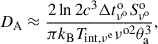
Due to these considerations, we set upper and lower limits on Tint. These limits are given in Table 1 and also plotted in Figure 1. It should be noted that Nair et al. (2019) utilizes an alternative population model (Lobanov et al. 2000) to find values of ![Mathematical equation: $ \log_{10}T_{\mathrm{int}}\mathrm{[K]}= 11.32_{-0.02}^{+0.01} $](/articles/aa/full_html/2025/11/aa56473-25/aa56473-25-eq20.gif) , which is two orders of magnitude larger than those found in this paper and more comparable to the variability-based estimates. Accelerating jets in the millimeter core region (e.g., Lee et al. 2016; Röder et al. 2025) and varying Tint with source variability (Homan et al. 2006) combined with a distribution of γj over multiple sources (e.g., Homan et al. 2021) may introduce additional offsets between the different population studies (Appendix B). Future experiments consisting of regular (e.g., less than monthly) multifrequency VLBI observations of a complete sample of sources may allow us to more concretely determine the potential frequency dependence of Tint as well as to resolve the offsets between different methods.
, which is two orders of magnitude larger than those found in this paper and more comparable to the variability-based estimates. Accelerating jets in the millimeter core region (e.g., Lee et al. 2016; Röder et al. 2025) and varying Tint with source variability (Homan et al. 2006) combined with a distribution of γj over multiple sources (e.g., Homan et al. 2021) may introduce additional offsets between the different population studies (Appendix B). Future experiments consisting of regular (e.g., less than monthly) multifrequency VLBI observations of a complete sample of sources may allow us to more concretely determine the potential frequency dependence of Tint as well as to resolve the offsets between different methods.
Frequency dependent constraints on Tint.
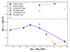 |
Fig. 1. Intrinsic brightness temperature, Tint, of AGNs obtained at different νo. Values with the label “pop” were obtained from a population analysis of Tvlb and βapp. Values with the label “var” were obtained utilizing flux density variability. All values were scaled to correspond to a disk source geometry. The dashed horizontal line corresponds to the Teq ≈ 5 × 10¹⁰ K of Readhead (1994). The values of Lee2014 are from Lee (2014), Nair2019 from Nair et al. (2019), Homan2021 from Homan et al. (2021), and Liodakis2018 from Liodakis et al. (2018), and they have been adjusted for the source geometry. |
5. Conclusions
We have investigated the Tint of the cores of AGNs utilizing both flux variability and a population analysis of Tvlb. During this process, we refined the equations in Hodgson et al. (2023) to properly account for the assumed source geometry, leading to a factor of approximately two lower value of Tint compared to the original equations. Assuming a uniform disk geometry, we placed upper and lower limits on log10Tint at various frequencies between 15 and 86 GHz. We were not able to constrain any frequency dependence on Tint. Resolution of the offsets between the different methods as well as more detailed investigation of the redshift and frequency dependence of Tint may be possible with tailored, regular (high) cadence (quasi-)simultaneous multifrequency observations of a complete sample of sources spanning a wide redshift range.
Acknowledgments
We thank the anonymous reviewer for valuable comments and suggestions that helped to improve the paper. This work was supported by the National Research Foundation of Korea (NRF) grant funded by the Korea government (MIST) (2020R1A2C2009003, RS-2025-00562700). This research has made use of data from the MOJAVE database that is maintained by the MOJAVE team (Lister et al. 2018) This study makes use of VLBA data from the VLBA-BU Blazar Monitoring Program (BEAM-ME and VLBA-BU-BLAZAR; http://www.bu.edu/blazars/BEAM-ME.html), funded by NASA through the Fermi Guest Investigator Program. The VLBA is an instrument of the National Radio Astronomy Observatory. The National Radio Astronomy Observatory is a facility of the National Science Foundation operated by Associated Universities, Inc.
References
- Adame, A. G., Aguilar, J., Ahlen, S., et al. 2025, JCAP, 2025, 021 [CrossRef] [Google Scholar]
- Boettcher, M., Harris, D. E., & Krawczynski, H. 2012, Relativistic Jets from Active Galactic Nuclei (Berlin: Wiley) [Google Scholar]
- Cheng, X. P., An, T., Hong, X. Y., et al. 2018, ApJS, 234, 17 [NASA ADS] [CrossRef] [Google Scholar]
- Cheng, X. P., An, T., Frey, S., et al. 2020, ApJS, 247, 57 [NASA ADS] [CrossRef] [Google Scholar]
- D’Agostino, R., & Pearson, E. S. 1973, Biometrika, 60, 613 [Google Scholar]
- de Witt, A., Jacobs, C. S., Gordon, D., et al. 2023, AJ, 165, 139 [NASA ADS] [CrossRef] [Google Scholar]
- Ghisellini, G., Padovani, P., Celotti, A., & Maraschi, L. 1993, ApJ, 407, 65 [Google Scholar]
- Guijosa, A., & Daly, R. A. 1996, ApJ, 461, 600 [Google Scholar]
- Hodgson, J. A., L’Huillier, B., Liodakis, I., Lee, S.-S., & Shafieloo, A. 2020, MNRAS, 495, L27 [Google Scholar]
- Hodgson, J. A., L’Huillier, B., Liodakis, I., Lee, S.-S., & Shafieloo, A. 2023, MNRAS, 521, L44 [Google Scholar]
- Homan, D. C., Kovalev, Y. Y., Lister, M. L., et al. 2006, ApJ, 642, L115 [NASA ADS] [CrossRef] [Google Scholar]
- Homan, D. C., Cohen, M. H., Hovatta, T., et al. 2021, ApJ, 923, 67 [NASA ADS] [CrossRef] [Google Scholar]
- Hovatta, T., Valtaoja, E., Tornikoski, M., & Lähteenmäki, A. 2009, A&A, 494, 527 [CrossRef] [EDP Sciences] [Google Scholar]
- Hsu, P.-C., Koay, J. Y., Matsushita, S., et al. 2023, MNRAS, 525, 5105 [Google Scholar]
- Jorstad, S. G., Marscher, A. P., Morozova, D. A., et al. 2017, ApJ, 846, 98 [Google Scholar]
- Kellermann, K. I., & Pauliny-Toth, I. I. K. 1969, ApJ, 155, L71 [NASA ADS] [CrossRef] [Google Scholar]
- Lee, S.-S. 2013, J. Korean Astron. Soc., 46, 243 [NASA ADS] [CrossRef] [Google Scholar]
- Lee, S.-S. 2014, J. Korean Astron. Soc., 47, 303 [NASA ADS] [CrossRef] [Google Scholar]
- Lee, S.-S., Lobanov, A. P., Krichbaum, T. P., et al. 2008, AJ, 136, 159 [Google Scholar]
- Lee, S.-S., Lobanov, A. P., Krichbaum, T. P., & Zensus, J. A. 2016, ApJ, 826, 135 [Google Scholar]
- Liodakis, I., Marchili, N., Angelakis, E., et al. 2017, MNRAS, 466, 4625 [NASA ADS] [CrossRef] [Google Scholar]
- Liodakis, I., Hovatta, T., Huppenkothen, D., et al. 2018, ApJ, 866, 137 [Google Scholar]
- Lister, M. L., Aller, M. F., Aller, H. D., et al. 2018, ApJS, 234, 12 [CrossRef] [Google Scholar]
- Lister, M. L., Homan, D. C., Hovatta, T., et al. 2019, ApJ, 874, 43 [NASA ADS] [CrossRef] [Google Scholar]
- Lister, M. L., Homan, D. C., Kellermann, K. I., et al. 2021, ApJ, 923, 30 [NASA ADS] [CrossRef] [Google Scholar]
- Lobanov, A. 2015, A&A, 574, A84 [NASA ADS] [CrossRef] [EDP Sciences] [Google Scholar]
- Lobanov, A. P., Krichbaum, T. P., Graham, D. A., et al. 2000, A&A, 364, 391 [NASA ADS] [Google Scholar]
- Nair, D. G., Lobanov, A. P., Krichbaum, T. P., et al. 2019, A&A, 622, A92 [NASA ADS] [CrossRef] [EDP Sciences] [Google Scholar]
- Pearson, T. J. 1995, in Very Long Baseline Interferometry and the VLBA, eds. J. A. Zensus, P. J. Diamond, & P. J. Napier, ASP Conf. Ser., 82, 267 [NASA ADS] [Google Scholar]
- Planck Collaboration VI. 2020, A&A, 641, A6 [NASA ADS] [CrossRef] [EDP Sciences] [Google Scholar]
- Readhead, A. C. S. 1994, ApJ, 426, 51 [Google Scholar]
- Riess, A. G., Yuan, W., Macri, L. M., et al. 2022, ApJ, 934, L7 [NASA ADS] [CrossRef] [Google Scholar]
- Röder, J., Wielgus, M., Lobanov, A. P., et al. 2025, A&A, 695, A233 [NASA ADS] [CrossRef] [EDP Sciences] [Google Scholar]
- Savolainen, T., Wiik, K., Valtaoja, E., & Tornikoski, M. 2006, A&A, 446, 71 [CrossRef] [EDP Sciences] [Google Scholar]
- Shapiro, S. S., & Wilk, M. B. 1965, Biometrika, 52, 591 [Google Scholar]
- Strauss, M. A., Huchra, J. P., Davis, M., et al. 1992, ApJS, 83, 29 [Google Scholar]
- Thompson, A. R., Moran, J. M., & Swenson, G. W. 2017, Calibration and Imaging (Cham: Springer International Publishing), 485 [Google Scholar]
- Tingay, S. J., Preston, R. A., Lister, M. L., et al. 2001, ApJ, 549, L55 [Google Scholar]
- Weaver, Z. R., Jorstad, S. G., Marscher, A. P., et al. 2022, ApJS, 260, 12 [NASA ADS] [CrossRef] [Google Scholar]
- Wiik, K., & Valtaoja, E. 2001, A&A, 366, 1061 [NASA ADS] [CrossRef] [EDP Sciences] [Google Scholar]
Appendix A: Deriving the causality-constrained angular diameter distance
A.1. Intensity, total flux density, and brightness temperature
The intensity of a source for the different geometries considered may be parameterized as follows (e.g., Thompson et al. 2017):
For a uniform disk with radius a,
 (A.1)
(A.1)
For a circular Gaussian with a linear FWHM  ,
,
 (A.2)
(A.2)
Finally, for an optically thin uniform sphere with radius a,
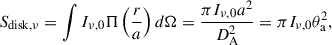
![Mathematical equation: $$ \begin{aligned} \frac{I_{\nu }\left(r\right)}{I_{\nu ,0}} = \sqrt{1-\left[\frac{r}{a}\right]^2}\Pi \left(\frac{r}{a}\right). \end{aligned} $$](/articles/aa/full_html/2025/11/aa56473-25/aa56473-25-eq24.gif) (A.3)
(A.3)
In the equations, r is the radial offset from the center, and Iν, 0 is the intensity at r = 0. The function Π(x) is defined such that
 (A.4)
(A.4)
To find the total flux density, Sν, that would be observed, we integrated over the full intensity distribution:
 (A.5)
(A.5)
Starting with a circular Gaussian, we have
 (A.6)
(A.6)
where we used  and θFWHM = lFWHM/DA. For a uniform disk, we have
 (A.7)
(A.7)
where θa = a/DA. For a uniform sphere,
![Mathematical equation: $$ \begin{aligned} S_{\rm sphere,\nu } =\int {I_{\nu ,0}\sqrt{1-\left[\frac{r}{a}\right]^2}\Pi \left(\frac{r}{a}\right)d\Omega } =\frac{2\pi I_{\nu ,0}a^2}{3D_{\rm A}^2} =\frac{2\pi I_{\nu ,0}}{3}\theta _{\rm a}^2. \end{aligned} $$](/articles/aa/full_html/2025/11/aa56473-25/aa56473-25-eq30.gif) (A.8)
(A.8)
The intensity of a source is commonly referenced to an equivalent blackbody temperature, i.e., the brightness temperature, Tb. In the Rayleigh-Jeans limit (hν≪kBTb), Iν ≈ 2kBν2Tb, ν/c2. Therefore, we have
 (A.9)
(A.9)
for a uniform disk with a radius of a,
 (A.10)
for a circular Gaussian with a FWHM of lFWHM, and
 (A.11)
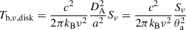
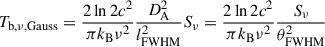
for a uniform sphere with a radius of a. The angular size (θa, θFWHM) of the source can be measured with VLBI. We denote such VLBI-measured brightness temperatures as Tvlb, ν.
We can also employ a = cΔt to define a “variability brightness temperature,” Tvar, ν. For a disk, this is
 (A.12)
and for a sphere,
 (A.13)
The total physical size of a Gaussian is not as well-defined and we do not consider the variability brightness temperature of a Gaussian source here.
We briefly consider the measurement of θa with VLBI. Modeling of VLBI data typically occurs in the “visibility plane”, i.e., the Fourier space of the image plane and the actual measurements made with VLBI. The visibilties corresponding to Equations (A.1), (A.2), (A.3) are as follows (e.g., Thompson et al. 2017):
For a uniform disk with radius a,
 (A.14)
For a circular Gaussian with linear FWHM  ,
,
 (A.15)
Finally, for an optically thin uniform sphere with radius a,
 (A.16)
In the equations, Jn is the Bessel function of the first kind. For the same value of V(0), a Gaussian source with FWHM lFWHM, a disk with diameter 2a ≈ 1.6lFWHM, and a sphere with diameter 2a ≈ 1.8lFWHM all have the same visibility FWHM (e.g., Pearson 1995). Without measurements at sufficiently long baselines such that we are able to observe the null points, and/or without sufficient signal-to-noise ratio, it may prove difficult to directly differentiate between the three geometries. Therefore, in the absence of sufficient data, we may consider model-fitting a Gaussian to the visibilities. Then, we may take the model-fit component to represent a Gaussian with FWHM lFWHM, a disk with radius a ≈ 0.8lFWHM, or a sphere with radius a ≈ 0.9lFWHM. Indeed, such an approximation was made in Hodgson et al. (2020, 2023) as well.
We could then determine approximations to Equations (A.9), (A.11) as follows:
For a uniform disk with radius a,
 (A.17)
and for an optically thin uniform sphere with radius a,
 (A.18)
For the same value of θFWHM, Tb, ν, disk ≈ 0.56Tb, ν, Gauss, and Tb, ν, sphere ≈ 0.67Tb, ν, Gauss (e.g., Tingay et al. 2001; Savolainen et al. 2006).
A.2. Relativistic corrections to Tb, ν
In total we can consider three frames of reference. We have the observer frame ℱo at zcos = 0, in which the measurements are made. We then have the host-galaxy frame ℱa of the AGN at redshift zcos. Finally we have the jet emission frame ℱe, moving at a speed β relative to ℱa according to the bulk jet speed. First we discuss transformations between ℱa and ℱe. Transformations between ℱa and ℱe are governed by special relativity. For Tvlb, ν we have (e.g., Boettcher et al. 2012)
 (A.19)
where we assumed Sν ∝ ν−α. For Tvar, ν we have
 (A.20)
where we assumed Sν ∝ ν−α and Δtν ∝ ν−η. Regardless of spectral shape (i.e., α) and frequency dependence of Δt (i.e., η), we have
 (A.21)
If we assume Tvlb, νee = Tvar, νee = Tint, νe where Tint, νe is some intrinsic brightness temperature of the source, we have Tvlb, νaa = δTint, νe and Tvar, νaa = δ3Tint, νe. It should be noted that these equations hold regardless of whether the source is a disk, Gaussian, or sphere.
The observables undergo further changes due to the cosmological evolution of the universe (transformations between ℱo and ℱa). Relevant to the discussion in this paper, we have νa/νo = Δto/Δta = Sνaa/Sνoo = (1+zcos). Due to such cosmological corrections, we have
 (A.22)
Combined with Equation (A.21), this leads to
 (A.23)
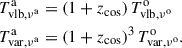
A.3. Variability angular diameter distance
The variability angular diameter distance may now be found as
 (A.24)
as in Hodgson et al. (2020). Following Hodgson et al. (2023), if we wish to instead use Tint to cancel out δ, we have
 (A.25)
For a disk or sphere, this reduces to
 (A.26)
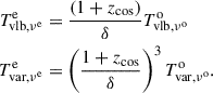
If we wish to rearrange the equations to assimilate the function of Tb, Gauss, we have
 (A.27)
where X ≈ 0.70 for a disk and X ≈ 0.74 for a sphere. Here θFWHM is the FWHM of the Gaussian function used to model the visibilities of the source. Equation (A.27) may also be used to calculate the intrinsic brightness temperature by rearranging Tint, νe to the left hand side and DA to the right hand side of the equation.
It should be noted that our equations slightly differ from Hodgson et al. (2023), who suggest that
 (A.28)
where θa = 0.8θFWHM for a disk and θa = 0.9θFWHM for a sphere (i.e., X ≈ 1.95 for a disk and X ≈ 1.37 for a sphere). The difference in the “geometrical correction factors” prescribed in Equation (A.28) from those derived in Equation (A.27) stems from the function of Tvlb used when canceling δ in Equation (A.24). Equation (A.28) corrects for the measured angular size (i.e., from θFWHM to θa) while approximating Tvlb, ν as Tb, ν, Gauss. Equation (A.27) accounts for the appropriate analytical functions of Tvlb, ν for the assumed geometry (i.e., Equations (A.9), (A.11) respectively for a disk and spherical emission region) as well. We find that compared to Equation (A.27), the use of Equation (A.28) overestimates DA by approximately a factor of 2.77 for a disk and 1.85 for a sphere, which, if left unaccounted for, results in a large systematic offset in DA (or equivalently, Tint).
Appendix B: Biases in the estimation of Tint
In the main text, we describe the expectation of a log-normal distribution, and no trend in Tint as a function of cadence. The two-point estimate of τi + 1, i relies on significant flux variability measurements with a cadence comparable to or better than the variability timescale of the flare in question. Estimates of τi + 1, i may be biased toward larger values, should the conditions not be met. As a simple test, we alternate the constraint on ti + 1 − ti to be less than 30 days, 50 days, 100 days, 500 days, and unconstrained. Values of log10Tint [K], as well as the sample average of log10Tint [K] (i.e., ⟨log10Tint [K]⟩), are given in Table B.1. Histograms of the estimated log10Tint [K] with ti + 1 − ti < 30 days may be found in Figure B.1. The black solid and dot-dashed vertical lines are the median and corresponding one-sigma confidence interval on log10Tint [K]. The red solid and dot-dashed horizontal lines are the same, but for ⟨log10Tint [K]⟩. Estimates of both log10Tint [K] and ⟨log10Tint [K]⟩ tend to be higher when the constraint on ti + 1 − ti changes from 30 days to unconstrained.
It should be noted that the number of individual sources that remain within each filter varies greatly (from 75 to 356 sources) for the 15 GHz data. This is primarily due to the varying (and somewhat lower) cadence of the MOJAVE observations. The number of sources does not change as much (37-38) at 43 GHz, due to the regular (bi-)monthly observations of the Boston University monitoring program. When repeating the analysis at 15 GHz with the source sample limited to the 75 sources that pass all 5 constraint sets, we find that the data-constraint-induced biases still exist (Table B.2). Values of log10Tint also tend to be higher with the 75 source sample. A paired sample t-test shows that the variation of log10Tint with different constraints on ti + 1 − ti is significant (p − value < 0.01) at both frequencies. This suggests that the estimates of log10Tint may be affected by (changes in) the source sample as well as observation cadence. Therefore, we refer to the values obtained with the constraint ti + 1 − ti < 30 days as upper limits on both the 15 GHz data and the 43 GHz data.
Additionally, we conducted a D’Agostino and Pearson’s test (DP test) and Shapiro-Wilk test (SW test) on the 15 and 43 GHz log10Tint samples to quantify deviations from a normal distribution. At 43 GHz, both DP and SW tests resulted in p-values > 0.1 for most ti + 1 − ti constraints. The only exception was the SW test combined with the 30-day constraint, resulting in a p-value of 0.0098. At 15 GHz, only the DP test with a 500-day constraint results in a p-value of > 0.05. All other cases result in p-values < 0.0129, with most less than 0.001. This suggests that while the distribution of log10Tint approximately follows a normal distribution at 43 GHz, there is a significant deviation from normality at 15 GHz.
Dependence of Tint on data constraints used.
Dependence of Tint on data constraints used (fixed sources).
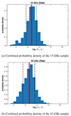 |
Fig. B.1. Estimated Tint at 15 GHz (upper row) and at 43 GHz (lower row). |
While the data suggests that we are currently cadence-limited, we briefly consider methods that may reduce the uncertainties associated with the variability analysis. The width of the distribution of Tint derived from variability is quite large, spanning a few orders of magnitude. A significant contributor to the large scatter is the large uncertainties associated with determining τi + 1, i. Such uncertainties may be reduced if we attempt to fit an e-folding timescale to multiple successive points (as in e.g., Hodgson et al. 2020) or through light curve decomposition, should the observation cadence and number of data points be sufficient. As a simple test, we repeat the analysis by calculating the e-folding timescale from the first and last measurement of segments with a continuous increase in flux density. We find that there are changes of Δlog10Tint[K] = −0.06 to +0.01 for the 15 GHz data and Δlog10Tint[K] = −0.08 to +0.02 for the 43 GHz data. Such variations are approximately an order of magnitude smaller than the uncertainty in log10Tint of σlog10Tint[K] ≈ 1. It could be that there are multiple, overlapping flares in the light curves of VLBI-resolved cores as well, the superpositon of which are affecting our e-folding timescale measurements. The current data does not have sufficient observation cadence for a robust light curve decomposition. Constraining a representative characteristic timescale per source (instead of using the values from each valid pair) may also help reduce the uncertainties.
Additional broadening of the distribution of Tint may come from systematics in our analysis. Of particular interest are potential source-dependent variations of Tint. The sources used in our analysis come from a wide range of redshifts, and therefore a wide range of νa. If there is indeed a frequency dependence of Tint, we would naturally expect the observed value of Tint to vary between sources. As Tint depends on the jet parameters of each source, there may be a non-negligible source-per-source variation as well. Given the current limitations, such variations are not apparent. It is possible that larger flares with longer variability timescales are in fact, sufficiently time-resolved, and may point toward two (or more) Tint populations. We will investigate the difference of Tint between the quiescent state and the larger flares in a separate, follow-up paper.
The distribution of Tvlb and βapp used in the population analysis of Section 2.2 is shown in Figure B.2. Blue circles represent constrained measurements of Tvlb. The dashed line represents the maximum βapp for a given bulk Lorentz factor (i.e., Equation (7)). Sources that fall under this line have a viewing angle smaller than the critical angle. The solid envelope corresponds to the expected value of βapp as a function of Tvlb for a bulk Lorentz factor of γj = 40 at 24 and 43 GHz, while γj = 35 at 86 GHz, where the value of γj at each frequency was determined based on the maximum βapp of the sources in the sample. The values of Tint found for a Gaussian source are given in Table B.3.
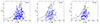 |
Fig. B.2. Estimated Tint at 24 GHz (left), 43 GHz (center), and 86 GHz (right) using a population study (see Section B for details). |
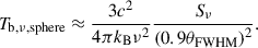
The values obtained from the population analysis in this paper are lower by approximately two orders of magnitude compared to Nair et al. (2019). We shortly discuss a couple of additional factors which may be biasing our results. βapp at all frequencies were determined using the maximum apparent speeds of jet components at 15 GHz. Homan et al. (2021) find that the maximum βapp does have the strongest correlation with the median Tvlb of the core (compared to the median βapp and βapp of the jet component closest to the core). However, multiple studies suggest acceleration of the jet plasma in the millimeter core region (e.g., Lee et al. 2016; Röder et al. 2025). In this case, βapp at the core should be lower than that implied by the jet components. To test the affect of this, we multiplied the observed βapp of each source by a random factor drawn from a uniform distribution between 0 to 1. For a Gaussian source model, we find that the nominal value of Tint is now  K,
K, 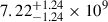 K, and
 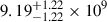 K at 24, 43, and 86 GHz, respectively. This is a factor of ∼2.4 increase compared to when we have used the maximum βapp directly (i.e, the values in Table B.3). A more realistic analysis may be done by modeling the jet acceleration as a function of distance from the jet base (as in, e.g., Röder et al. 2025). However, we find it unlikely that offsets of βapp would fully account for the two orders of magnitude difference.
Population study estimates of Tint.
Source variability may also affect the value of Tint. Homan et al. (2006) found that while Tint estimated for a "median-low brightness temperature state" is (for a Gaussian source model) Tint ≈ 3 × 10¹⁰ K, it could increase to Tint > 2 × 10¹¹ K when using the maximum observed brightness temperature, with the lower limit coming from unresolved cores. This suggests that there may be two populations of Tint, with the average/low state close to the equipartition brightness temperature (Readhead 1994), and the active/high state near the inverse Compton limit (Kellermann & Pauliny-Toth 1969). Nair et al. (2019) assumes a common γj over all sources instead of utilizing per-source βapp values. Further evaluation of the affect of a distribution of γj (as found in, e.g., Homan et al. 2021) on the analysis of Nair et al. (2019), as opposed to the use of a common value of γj over all sources, may also further reduce the offsets between the two methods.
Appendix C: Tint of the flaring component in 3C 84
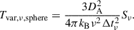
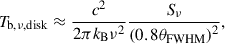
Hodgson et al. (2023) estimate Tint for a flaring component as Tint ∼ 1011 K at the peak of the flare. We recalculate this using the updated equations for Tint given in this paper (i.e., Equation (5)). We adopt Sνoo = 15.68 ± 1.53 Jy, 0.5θFWHM = 0.20 ± 0.02 mas, Δtνoo = 146 ± 5 days from Hodgson et al. (2020) and z = 0.0176 from Strauss et al. (1992). Taking Ωm = 0.315, ΩΛ = 0.685, H0 = 67.4 km/s/Mpc (Planck Collaboration VI 2020), we find 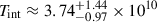 K when assuming a disk geometry and
 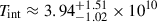 K when assuming a spherical geometry. We see that once appropriately accounting for source geometry, the intrinsic brightness temperature of the component is consistent with the equipartition brightness temperature limit of Teq ≈ 5 × 10¹⁰ K (Readhead 1994). It can be inferred that at the peak of the radio flare, the jet component may have been in equipartition between the magnetic and kinetic energy densities. The Doppler factor is found to be δ ≈ 1.12 ± 0.12 for a sphere and
  for a disk. As with Hodgson et al. (2023), we find that the values of δ are consistent with no Doppler boosting (i.e., δ = 1). The values of Tint and δ derived for different geometrical models, as well as for H0 = 73.04 km/s/Mpc (Riess et al. 2022) are summarized in Table C.1.
The Tint and δ of the jet component of 3C 84.
All Tables
All Figures
|
Fig. 1. Intrinsic brightness temperature, Tint, of AGNs obtained at different νo. Values with the label “pop” were obtained from a population analysis of Tvlb and βapp. Values with the label “var” were obtained utilizing flux density variability. All values were scaled to correspond to a disk source geometry. The dashed horizontal line corresponds to the Teq ≈ 5 × 10¹⁰ K of Readhead (1994). The values of Lee2014 are from Lee (2014), Nair2019 from Nair et al. (2019), Homan2021 from Homan et al. (2021), and Liodakis2018 from Liodakis et al. (2018), and they have been adjusted for the source geometry. |
| In the text | |
|
Fig. B.1. Estimated Tint at 15 GHz (upper row) and at 43 GHz (lower row). |
| In the text | |
|
Fig. B.2. Estimated Tint at 24 GHz (left), 43 GHz (center), and 86 GHz (right) using a population study (see Section B for details). |
| In the text | |
Current usage metrics show cumulative count of Article Views (full-text article views including HTML views, PDF and ePub downloads, according to the available data) and Abstracts Views on Vision4Press platform.
Data correspond to usage on the plateform after 2015. The current usage metrics is available 48-96 hours after online publication and is updated daily on week days.
Initial download of the metrics may take a while.