| Issue |
A&A
Volume 703, November 2025
|
|
|---|---|---|
| Article Number | A31 | |
| Number of page(s) | 11 | |
| Section | Stellar structure and evolution | |
| DOI | https://doi.org/10.1051/0004-6361/202556586 | |
| Published online | 31 October 2025 | |
Asteroseismology of 35 Kepler and TESS δ Scuti stars near the red edge of the instability strip
The limitations of δ Scuti stars for dating open clusters
Departamento de Física y Química, IES Levante, Avenida Italia s/n, 11205 Algeciras, Spain
⋆ Corresponding author: This email address is being protected from spambots. You need JavaScript enabled to view it.
Received:
24
July
2025
Accepted:
3
September
2025
Abstract
Aims. The aim of this work is to determine the maximum ages that can be unambiguously established for δ Sct stars using seismic observables and by extension the oldest open clusters that can be dated using this type of star.
Methods. I estimated the large frequency separation using various techniques applied to two samples of δ Sct located near the red edge of the instability strip. One sample consists of 18 targets observed by the Kepler mission, and the other comprises 17 targets observed by TESS. I employed a grid of stellar models representative of typical δ Sct parameters, incorporating mass, metallicity, and rotation as independent variables, and computed the first eight radial modes for each model. Using the observed spectroscopic temperature and the estimated large separation, I estimated the age of each star by fitting a weighted probability density function to the age distribution of the models that best match the seismic constraints.
Results. To evaluate the performance of the fitting method, it was applied to a synthetic population of 20 δ Sct stars with varying metallicities and ages, generated by randomly selecting models. The analysis indicates that δ Sct stars older than 1 Gyr but that have not yet reached the terminal-age main sequence can in principle be reliably age dated. Nevertheless, when the method is applied to the observational sample, only three out of the 35 stars considered marginally exceed an estimated age of 1 Gyr.
Conclusions. From these results, I can say that open clusters older than approximately 1 Gyr cannot be reliably dated using the asteroseismology of δ Sct stars with 1D models, at least not without a more complete treatment of convection and a non-linear treatment of rotation.
Key words: asteroseismology / stars: variables: delta Scuti / open clusters and associations: general
© The Authors 2025
 Open Access article, published by EDP Sciences, under the terms of the Creative Commons Attribution License (https://creativecommons.org/licenses/by/4.0), which permits unrestricted use, distribution, and reproduction in any medium, provided the original work is properly cited.
This article is published in open access under the Subscribe to Open model. This email address is being protected from spambots. You need JavaScript enabled to view it. to support open access publication.
1. Introduction
Within the Hertzsprung–Russell (HR) diagram, the classical instability strip (IS) encompasses several types of pulsating stars. The δ Sct are Population I stars of spectral types A2 to F2, are located near the main sequence (MS), and have effective temperatures ranging from approximately 6400 K to 8600 K (Breger 2000; Rodríguez & Breger 2001; Aerts et al. 2010; Uytterhoeven et al. 2011). They occupy an intriguing region of the HR between low-mass stars with radiative cores and thin convective envelopes (M ≲ 2 M⊙) and more massive stars with convective cores and radiative envelopes (M ≳ 2 M⊙).
The study of δ Sct stars provides valuable constraints on models of stellar structure and evolution, as physical properties such as the internal rotation and the size of the convective core play a key role in shaping the evolutionary paths of intermediate- and high-mass stars (Maeder 2009; Meynet et al. 2013). They can exhibit dozens to hundreds of radial and non-radial pulsation modes, with periods ranging from approximately 15 minutes to 8 hours (Uytterhoeven et al. 2011; Holdsworth et al. 2014). These oscillations are excited by the κ-mechanism operating in the He II partial ionisation zone (Cox 1963). Typically, these stars are fast rotators (Royer et al. 2007). As they evolve, their pulsation modes shift towards lower frequencies, which in the HR diagram corresponds to a movement towards the red, or cooler, edge of the IS. In this region, δ Sct overlap with γ Dor variables, which pulsate at lower frequencies excited by a convective blocking mechanism (Guzik et al. 2000; Dupret et al. 2005).
Detecting modes in γ Dor stars is challenging due to their closely spaced frequencies, which require long-duration, high-resolution observations on the order of 90 days to resolve them (Kurtz 2022). The advent of space-based photometry from the Kepler (Koch et al. 2010) and TESS (Ricker et al. 2014) missions has led to substantial progress in the asteroseismology of γ Dor stars (Van Reeth et al. 2015).
Determining the red edge of the IS remains a significant challenge, both theoretically and observationally. From a theoretical standpoint, models must incorporate time-dependent convection (TDC) to account for the coupling between oscillations and convection in the stellar envelope. Within the framework of the mixing length theory (MLT; Unno 1967), Xiong & Deng (2001) derived a theoretical red edge for radial modes using the non-local TDC formulation of Xiong et al. (1998). Similarly, Grigahcene et al. (2004) and Dupret et al. (2005) computed theoretical blue and red edges for both radial and non-radial modes, employing the TDC formalism developed by Gabriel (1996).
The location of the IS is highly sensitive to the choice of the free parameter α in the TDC treatment. According to Dupret et al. (2005), values of α between 1.8 and 2.0 yield better agreement with observational data. Ideally, a grid of models allowing for variation in this parameter would be constructed, especially near the terminal-age main sequence (TAMS). Houdek & Dupret (2015) provide a comprehensive summary of recent advances in this area.
From an observational standpoint, since the release of data from the Kepler space mission, evidence has emerged for the existence of hybrid stars exhibiting pulsations characteristic of both δ Sct and γ Dor stars (Uytterhoeven et al. 2011). This observational confirmation supported the theoretical predictions of Dupret et al. (2005). These hybrid stars display high-frequency acoustic modes (p-modes), typical of δ Sct stars, alongside low-frequency buoyancy modes (g-modes), typical of γ Dor stars. The interaction between these mode types occurs near the boundary separating the convective core from the radiative envelope, giving rise to the phenomenon of avoided crossings, where p- and g-modes of similar frequencies couple and exchange characteristics. It should be noted that clear evidence of avoided crossings has not been detected in the observed spectra of δ Sct in the same way as in solar-like stars.
To facilitate the classification of δ Sct and γ Dor stars, Grigahcène et al. (2010) proposed a frequency cut-off at 5 d−1. However, this limit is based more on statistical considerations than on physical theory. In Gautam et al. (2025), the authors show that δ Sct models near the zero-age main sequence (ZAMS) have g-modes around 20 d−1. The classification becomes even more complex with the discovery of a significant fraction of stars located within the IS that do not exhibit any pulsations. In Murphy et al. (2019), the edges of the IS were redefined based on the pulsator fraction in a sample of 15 000 A- and F-type stars.
In summary, the red edge of the IS is a theoretically and observationally challenging boundary to define. Around this region, two types of pulsating stars coexist, often displaying oscillation modes with similar frequencies but differing physical origins, complicating both their identification and seismic modelling.
One of the key seismic indicators is the large frequency separation (Δν), defined as the difference between acoustic modes of the same spherical degree and consecutive radial orders. This parameter is directly related to the mean density and surface gravity of the star, an approach previously applied to solar-like stars. Identifying these regular spacings between consecutive radial modes is challenging due to the presence of avoided crossings and the typically rapid rotation of δ Sct stars. Nevertheless, studies by García Hernández et al. (2013, 2015, 2017), Paparó et al. (2016), Michel et al. (2017) and Bedding et al. (2020) have found evidence of periodicities in the frequency spectra of δ Sct observed with CoRoT, Kepler, and TESS.
In Pamos Ortega et al. (2022, 2023) (hereafter Paper I and Paper II, respectively), we used the large separation observed in a sample of δ Sct to date three young open clusters with different metallicities and ages: α Persei, Trumpler 10, and Praesepe. We also employed the νmax–Teff scaling relation proposed by Barceló Forteza et al. (2020). However, some authors, such as Bedding et al. (2023), have questioned the applicability of this relation to δ Sct stars. The main concern lies in the complexity of their power spectra, which do not conform well to a Gaussian profile as observed in solar-type stars with stochastically excited oscillations and a well-defined maximum. In addition, Murphy et al. (2024) analysed the νmax–Teff relation in the young stellar association Cep Her, and they claim that this relation is unreliable, even for stars younger than approximately 100 Myr. Nevertheless, the independent scaling relations proposed by Barceló Forteza et al. (2020) and Hasanzadeh et al. (2021) were derived from sufficiently large and homogeneous samples of pure δ Sct stars. Although the dispersion in the relation is significant, it can still serve as a useful constraint for stellar models via the effective temperature, particularly in cases where the oscillation envelope is narrow and contains tightly clustered acoustic modes. This behaviour is more typical of young δ Sct located near the ZAMS or in the early stages of the MS. In contrast, for more evolved δ Sct along the MS, the νmax–Teff relation becomes less reliable due to an increased dispersion. For this reason, I chose to use available spectroscopic temperatures to constrain the models.
Many intermediate-mass stars exhibit moderate to high rotation rates, which further complicates the identification of observed oscillation modes. Under the assumption of uniform rotation and using first-order perturbation theory, the rotational splitting of a mode frequency, ωn, ℓ, in azimuthal order, m, is described by the equation ωn, ℓ, m = ωn, ℓ + m(1 − Cn, ℓ)Ω, where Ω is the rotation frequency and Cn, ℓ is the Ledoux constant, accounting for the influence of the Coriolis force. Rotation thus lifts the degeneracy of the mode ωn, ℓ, producing a multiplet of (2ℓ+1) distinct frequencies corresponding to different values of m for a fixed value of ℓ. In the case of high-order p-modes, the Ledoux constant is approximately zero (Aerts et al. 2010). Under these conditions, the resulting multiplets, comprising components with m = −ℓ, − ℓ + 1, ...0...ℓ − 1, ℓ, constitute a useful seismic observable for determining the stellar envelope’s rotation frequency independently of the equilibrium model. In Paper I and Paper II, these frequency multiplets were also used as a seismic diagnostic to estimate the rotation rate and constrain the stellar models in cases where such structures could be reliably detected.
Oscillations in rapidly rotating stars cannot be accurately described using spherical harmonics. More sophisticated perturbative approaches have been developed incorporating the Coriolis force up to second- and third-order terms in frequency calculations based on 1D equilibrium models (see Mirouh 2022, for a review of the effects of rapid rotation on mode geometry). In Paper I and Paper II, we employed a perturbative method up to the third order, accounting for stellar deformation and near-degeneracy effects, as developed by Suárez et al. (2002) and implemented in the FILOU code (Suárez & Goupil 2008), to compute oscillation modes across our model grids. However, since these phenomena are not relevant to the present analysis and considering the higher computational cost associated with FILOU, the GYRE code (Townsend & Teitler 2013) has been selected for this work as a more efficient alternative. As the present oscillation models consider only radial acoustic modes (Sect. 4), rotational multiplets were not employed as constraints in the model fitting process.
Building on the research presented in Paper I and Paper II, this work further refines the conditions under which δ Sct stars and the open clusters that host them can be reliably dated. I analyse the frequency content of a sample of δ Sct observed in various sectors by the Kepler and TESS missions, specifically focusing on those located near the red edge of the IS. There, the oldest δ Sct stars still on the MS but that have not yet reached the TAMS can be found. This is notable, as frequency analyses become too complex to allow for reliable age determination when a star reaches the TAMS. The primary objective is to estimate their ages and to determine an upper limit for the age of an open cluster that can be dated using δ Sct asteroseismology.
The structure of this paper is as follows: In Sect. 2 I describe the selection criteria for the stellar samples. In Sect. 3 I outline the frequency analysis methodology. Sect. 4 provides details on the construction of the model grid used in this work. In Sect. 5 I show the goodness of the method through a group of 20 simulated δ Sct stars. Sect. 6 presents the results obtained from the statistical treatment of the models for the stellar samples. Finally, in Sect. 7 I summarise the main conclusions of the study.
2. The samples
I began by identifying candidate δ Sct located as close as possible to the red edge of the IS. For this purpose, I consulted the catalogues of Murphy et al. (2019) and Stassun (2019) (hereafter M2019 and S2019, respectively), which include extensive samples of stars observed by the Kepler and TESS missions, respectively. I selected stars with effective temperatures between 6500 K and 7500 K, and metallicities in the range [Fe/H] = –0.3 to +0.3.
An additional selection criterion was the availability of short-cadence light curves (≃2 minutes) in PDCSAP FLUX from specific Kepler and TESS sectors, made accessible through the TESS Asteroseismic Science Consortium1 (TASC). It resulted in a sample of 64 candidates from Kepler and 53 from TESS. Figure 1 shows the location of these stars in the HR diagram. For consistency with the underlying data, I adopted the IS boundaries as defined by Murphy et al. (2019).
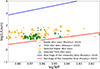 |
Fig. 1. Hertzsprung–Russell diagram showing 64 δ Sct candidates observed in various Kepler sectors (orange) and 53 δ Sct candidates observed in TESS sectors (green) all located near the red edge of the instability strip. Targets from both samples selected for seismic analysis are highlighted with circles. |
Once the oscillation frequencies were extracted using MULTIMODES2, the open-source code developed in Paper I, I visually inspected the periodograms of all the candidate stars. This step was crucial to discard stars exhibiting oscillation spectra with clear signs of avoided crossings or indications of high rotational velocity, both of which tend to blend oscillation modes and hinder mode identification.
I retained only those stars whose frequency spectra displayed well-separated p-modes clearly distinguishable from the low-frequency signals typically associated with convection or rotation. These selected targets, 18 from the Kepler sample and 17 from TESS, are marked with circles in Fig. 1. Tables A.1 and A.2 in Appendix A list the main parameters of each selected star in each sample.
Among the listed parameters, I highlight the projected rotational velocity, vsini, compiled from various sources. Candidates with v ⋅ sin i > 120 km s−1 and periodograms dominated by a complex mix of low and high frequencies were excluded from the final analysis, as their seismic modelling would be unreliable with the methods used here.
Figure 2 illustrates two discarded cases. The top panel shows the periodogram for KIC 6123324, where most of the detected frequencies lie below 10 d−1, suggesting that rotational or convective processes dominate its variability. The bottom panel shows the periodogram of TIC 121729614, which presents a dense forest of frequencies, both low and high, along with evidence of avoided crossings. Its high projected rotational velocity, 260 km s−1 (Niemczura et al. 2015)), supports this interpretation. Although the stars in each group may exhibit a wide range of metallicities, both samples can provide an empirical upper limit on the age at which δ Sct stars, and by extension the open clusters that host them, can be reliably dated through asteroseismology.
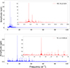 |
Fig. 2. Top: Periodogram of KIC 6123324. Bottom: Periodogram of TIC 121729614. |
3. The seismic analysis
After extracting the oscillation frequencies for each star in both samples using the MULTIMODES code, I estimated the large frequency separation (Δν) following the same techniques described in Paper I and Paper II (and references therein). As an illustrative example, the top panel of Fig. 3 shows the estimated Δν for KIC 8827281. Each figure is divided into two panels: the left panel presents the Δν estimation obtained using three different methods, the Fourier transform, the autocorrelation function, and the frequency separation histogram, while the right panel displays the corresponding échelle diagram. The results for the full set of selected targets are shown in a Zenodo public repository (https://doi.org/10.5281/zenodo.17067341).
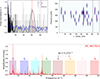 |
Fig. 3. Top: Estimated large separation for KIC 8827821, Δν = 61 μHz = 5.27 d−1. Top left: Fourier transform (FT), autocorrelation (AC), and the histogram of frequency differences (HFD). Top right: Echélle diagram (ED). Bottom: Frequency ranges corresponding to radial modes with radial orders n = 1 to n = 8 based on the estimated large separation. |
In addition to the large separation, I used the available spectroscopic temperature, taken from the M2019 catalogue for the Kepler sample and from the S2019 catalogue for the TESS sample, to constrain the stellar models computed in this work. These constraints allowed me to compare the observed frequencies with those predicted for radial modes with orders n = 1 to n = 8. The objective was to define a frequency range for each radial mode within the observed spectrum. This approach provides greater confidence in the Δν estimates and allows for tighter constraints on stellar ages in the next step of the analysis.
The bottom panel of Fig. 3 illustrates this method. There, the coloured rectangles indicate the frequency ranges in which each of the first eight radial modes is expected to lie, based on the estimated Δν for KIC 8827821.
The corresponding radial mode frequency ranges for all the selected stars in the Kepler and TESS samples are available in https://doi.org/10.5281/zenodo.17067341. The specific numerical values used in this analysis are also provided in Tables A.3 and A.4 in Appendix B.
4. The grid
To characterise δ Sct stars in the MS, I computed a grid of stellar models using MESA, version r24081 (Paxton 2019), evolving each model up to the TAMS. As configured by default, the code was allowed to determine the optimal time step between consecutive models during the evolution. The models were calculated based on the set of independent parameters listed in Table 1. The nuclear reaction network used was pp_and_cno_extras.net, following the prescriptions of Murphy et al. (2023).
Parameters of the stellar model grids computed with the MESA code.
At the ZAMS, the initial chemical composition satisfies X + Y + Z = 1. For a fixed value of hydrogen mass fraction X, increasing metallicity Z results in a corresponding decrease in helium fraction Y. The models incorporate differential rotation, with rotation initiated at the ZAMS. The initial angular velocity to critical velocity ratios were chosen in the range 0.1Ωc to 0.5Ωc, avoiding higher values that exceed the applicability limits of the perturbative approach and adhering to the assumptions underlying the GYRE pulsation code.
Convective core overshooting was not included. In Paper II, we tested exponential overshooting values of f0 = 0.002 and f = 0.022 and found no significant impact on the age uncertainties of Trumpler 10 and Praesepe. In the present study, the vast majority of stars in the sample, if not all, have not yet reached the TAMS, as inferred from their positions in the HR diagram, where the effects of the overshooting become significant. Moreover, the primary objective of this work is not to provide a precise characterisation of each individual star.
The atmospheric boundary condition was set using MESA’s default configuration, adopting a fixed Eddington T-τ relation (Eddington 1926). The choice of an atmospheric model has a negligible impact on the oscillation frequencies considered here, which are excited at sufficiently deep layers within the radiative envelope.
Parameters of 20 simulated δ Sct stars.
I computed the oscillation modes using GYRE, version 7.2.1. As explained in Sect. 2, the focus of this study is on stars that predominantly exhibit p-modes rather than g-modes. Accordingly, I limited the computation to the first eight radial p-modes. In this regime, the Coriolis force has a negligible effect on the eigenfunctions of the modes, and the influence of centrifugal distortion is even smaller. Under these conditions, the use of 1D oscillation models, enabled by the close coupling between the equilibrium models computed with MESA and the oscillation models computed with GYRE, is fully justified.
The oscillation computations employed the second-order Gauss–Legendre Magnus integration scheme (MAGNUS_GL2). I performed frequency scans in the range 5–100 d−1 using a grid of 100 frequency points. To reproduce the expected distribution of p-modes, I selected a linear frequency grid (grid_type = ‘LINEAR’), which is appropriate for modes that are approximately equally spaced in frequency at high radial orders. It is well established that radial modes are not strictly equally spaced, with the first four modes typically lying closer together than the subsequent four. Accordingly, the large frequency separation was determined as the average of the separations between consecutive radial modes in the range n = 5 to n = 8. For refining the mesh of integration points around each trial frequency, I adopted the recommended GYRE parameters: wosc = 10, wexp = 2, and wctr = 10.
5. Testing the method with a group of 20 simulated δ Sct stars
The statistical treatment applied here follows the same methodology as in Paper II. As a reminder, a major source of bias in the computed models arises from the oversampling of very young models produced by MESA. This effect is mitigated by applying a weighting factor proportional to the time step between consecutive models along the evolutionary track. The impact is most relevant near the PMS and the ZAMS, while it becomes negligible for more evolved models on the MS.
Using the updated weighted probability density function (WPDF), I computed histograms of the constrained models and fitted a Gaussian distribution to them, evaluating the goodness of fit using the Pearson chi-squared statistic, χ2. Prior to applying the method to the observational samples, its reliability was assessed using simulated stars. To do so, I selected 20 models from the previously computed grid (Table 2) covering effective temperatures between 6500 K and 7500 K, and spanning a range of metallicities and ages.
For each simulated star, the effective temperature and the large frequency separation were adopted as observational constraints. In all cases, the effective temperature was assigned an uncertainty of 150 K, a value representative of many stars in the Kepler and TESS samples. For the large frequency separation, an uncertainty of 2 μHz was assumed, corresponding to the average uncertainty measured in real stars. Treating the objects as field stars, the metallicity was not included as a constraint since this parameter is typically subject to large uncertainties. Conversely, if the stars are assumed to belong to a cluster of known metallicity, this parameter can be incorporated to further restrict the models. For each case, histograms and WPDFs were computed (Figure 4). The resulting fits, those constrained by metallicity (red) and those unconstrained (blue), were compared with the true age of the simulated star (green line). This procedure provided an estimate of the intrinsic uncertainty associated with the fitting method.
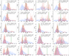 |
Fig. 4. Histograms and WPDFs of 20 simulated stars with different metallicities. The colours indicate when Z is used (red) and not used (blue) as an observational constraint. The green solid line represents the real age of the model. |
Several conclusions can be drawn from this study. First, as expected, the distributions are more Gaussian-like when metallicity is not used as a constraint. Second, in only eight stars (numbers 1, 2, 3, 4, 5, 8, 14, and 20), constraining the models by metallicity yields ages closer to the true values, primarily in the subsolar regime. However, the corresponding histograms do not exhibit Gaussian distributions, owing to the insufficient number of models, either because the stellar mass lies near the lower limit of the grid or because the rotation rate approaches the upper boundary. Third, the fits obtained for solar metallicity are very similar, as expected, given that the grid was designed with Z ≃ 0.020 as the average value. Finally, for three of the 20 stars (numbers 13, 18, and 19), no reliable age determination was possible within the adopted uncertainties. Notably, these correspond to some of the oldest stars in the sample. Near the TAMS, the grid density becomes insufficient to achieve a good fit consistent with a normal distribution. Nevertheless, stars numbered 2, 9, and particularly 16 – each older than 1 Gyr – have been dated with remarkable precision. This result demonstrates that, within this grid, reliable age determinations can be extended to stars well beyond this threshold.
This simulation supports a key conclusion of the study: Metallicity should not be used as a constraint in the modelling of individual stars with the present grid. It is not a reliable observable, as its reported values vary significantly across different sources and catalogues. In addition, the number of models in the grid becomes insufficient near the extreme values, preventing the construction of normal distributions that can be reliably fitted. A more finely sampled metallicity grid would therefore be required for modelling of individual stars or in cases where the objective is to determine the age of a cluster.
6. Results and discussion
Figure 5 shows the constrained models in Δν and Teff for the Kepler (left panel) and the TESS (right panel) samples. In addition, Figure 6 shows the age histogram, the WPDF, and the estimated age for KIC 8827821. The complete set of histograms for the Kepler and TESS samples is available at https://doi.org/10.5281/zenodo.17067341. The parameters corresponding to each of the modelled stars are shown in Tables A.5 and A.6 in the Appendix C.
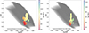 |
Fig. 5. Left panel: Seismically constrained stellar models for the Kepler sample of δ Sct stars using a large separation, spectroscopic temperatures, and metallicities. Right panel: Same as left but for the TESS sample. |
The ages of the Kepler sample range from 404 ± 236 Myr, corresponding to the star KIC 10686752, to 1095 ± 246 Myr, corresponding to KIC 7106205. For the TESS sample, the range spans from 331 ± 240 Myr (TIC 69025963) to 1029 ± 241 Myr (TIC 398733851). The models are consistent in metallicity, with all of them exhibiting values around Z = 0.020–0.022. This uniformity near the solar value results from the computed models spanning Z = 0.010–0.030. It is likely that several stars have not been accurately modelled, given the expected diversity in metallicity. Nevertheless, this does not significantly affect the estimated average age for each sample, as I have shown in Sect. 5.
With these results, I conclude that the oldest stars that can be reliably dated using this technique, at least not with 1D models, and without a more complete treatment of convection and a non-linear treatment of rotation barely reach 1000 Myr. To further support this claim, in Fig. 7 I show the MS evolution of radial modes (ℓ = 0) and non-radial modes (ℓ = 1, 2) for an evolutionary track with M = 1.64 M⊙, solar-like metallicity (Z = 0.018), and Ω/Ωcrit = 0.10, which are representative values of the Kepler sample. As age increases beyond 600 Myr, non-radial modes of different orders begin to interact and overlap. Around 1000 Myr, this mixing extends to fifth-order modes, significantly affecting the determination of the large separation. In addition to the effects of rotation and the avoided crossings phenomenon, where p-modes mix with g-modes, the overlapping of p-modes themselves further complicates the estimation of the large separation. Although the sample is not large enough to draw a definitive statistical limit, I think that these factors are sufficient to prevent old δ Sct from being dated since the large separation becomes indeterminable and cause mode identification in the frequency spectrum to no longer be feasible.
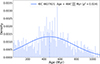 |
Fig. 6. Age histogram and WPDF derived from the seismically constrained models for KIC 8827821. The Gaussian fit and the corresponding χ2 value are also shown. |
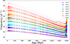 |
Fig. 7. Evolution of the oscillation mode frequencies along the MS for radial orders between n = 1 and n = 8, and degrees ℓ = 0, 1, 2, corresponding to an evolutionary track with M = 1.64 M⊙, metallicity Z = 0.018, and a rotation rate of Ω/Ωcrit = 0.10. |
7. Conclusions
One-dimensional stellar models that neglect rapid rotation and lack a proper treatment of convection, such as those used in the present research, are insufficient for reliably determining the ages of δ Sct stars older than 1 Gyr. A statistical analysis performed on a synthetic stellar sample suggests that such age determination could, in principle, be achieved if a sufficiently large number of models is available to yield a normally distributed histogram. However, when applied to the observed sample, only three stars, KIC 7106205, TIC 394015973, and TIC 398733851, exceed this age threshold. This limitation is likely attributable to the inability to obtain reliable estimates of the large frequency separation for stars excluded during the initial selection process.
Data availability
Plots of the large frequency separation estimates, radial mode ranges, and age histograms for each star are publicly available at Zenodo (https://doi.org/10.5281/zenodo.17067341).
Acknowledgments
I appreciate the comments and questions from the anonymous referee, because they have contributed to improving the paper. I also appreciate the work of Dr. Juan Carlos Suárez and Dr. Antonio García Hernández, from the University of Granada, who were my thesis project directors, which I completed in December 2024.
References
- Aerts, C., Christensen-Dalsgaard, J., & Kurtz, D. W. 2010, Asteroseismology (Springer Science+Business Media B.V.) [Google Scholar]
- Balona, L. A., Baran, A. S., Daszyńska-Daszkiewicz, J., & De Cat, P. 2015, MNRAS, 451, 1445 [Google Scholar]
- Barceló Forteza, S., Moya, A., Barrado, D., et al. 2020, A&A, 638, A59 [NASA ADS] [CrossRef] [EDP Sciences] [Google Scholar]
- Bedding, T. R., Murphy, S. J., Hey, D. R., et al. 2020, Nature, 581, 147 [NASA ADS] [CrossRef] [Google Scholar]
- Bedding, T. R., Murphy, S. J., Crawford, C., et al. 2023, ApJ, 946, L10 [NASA ADS] [CrossRef] [Google Scholar]
- Breger, M. 2000, ASP Conf. Ser., 210, 3 [NASA ADS] [Google Scholar]
- Cox, J. P. 1963, ApJ, 138, 487 [NASA ADS] [CrossRef] [Google Scholar]
- Dupret, M. A., Grigahcène, A., Garrido, R., Gabriel, M., & Scuflaire, R. 2005, A&A, 435, 927 [NASA ADS] [CrossRef] [EDP Sciences] [Google Scholar]
- Eddington, A. S. 1926, The Internal Constitution of the Stars (Cambridge: Cambridge University Press) [Google Scholar]
- Frasca, A., Molenda-Żakowicz, J., De Cat, P., et al. 2016, A&A, 594, A39 [CrossRef] [EDP Sciences] [Google Scholar]
- Gabriel, M. 1996, Bull. Astron. Soc. India, 24, 233 [Google Scholar]
- García Hernández, A., Moya, A., Michel, E., et al. 2013, A&A, 559, A63 [NASA ADS] [CrossRef] [EDP Sciences] [Google Scholar]
- García Hernández, A., Martín-Ruiz, S., Monteiro, M. J. P. F. G., et al. 2015, ApJ, 811, L29 [Google Scholar]
- García Hernández, A., Suárez, J. C., Moya, A., et al. 2017, MNRAS, 471, L140 [CrossRef] [Google Scholar]
- Gautam, A., Murphy, S. J., & Bedding, T. R. 2025, arXiv e-prints [arXiv:2507.03561] [Google Scholar]
- Gebran, M., Farah, W., Paletou, F., Monier, R., & Watson, V. 2016, A&A, 589, A83 [NASA ADS] [CrossRef] [EDP Sciences] [Google Scholar]
- Grigahcene, A., Dupret, M. A., Garrido, R., Gabriel, M., & Scuflaire, R. 2004, CoAst, 145, 10 [Google Scholar]
- Grigahcène, A., Antoci, V., Balona, L., et al. 2010, ApJ, 713, L192 [Google Scholar]
- Guzik, J. A., Kaye, A. B., Bradley, P. A., Cox, A. N., & Neuforge, C. 2000, ApJ, 542, L57 [Google Scholar]
- Hasanzadeh, A., Safari, H., & Ghasemi, H. 2021, MNRAS, 505, 1476 [NASA ADS] [CrossRef] [Google Scholar]
- Holdsworth, D. L., Smalley, B., Gillon, M., et al. 2014, MNRAS, 439, 2078 [NASA ADS] [CrossRef] [Google Scholar]
- Hou, W., Luo, A., Yang, H., et al. 2015, MNRAS, 449, 1401 [CrossRef] [Google Scholar]
- Houdek, G., & Dupret, M.-A. 2015, Liv. Rev. Sol. Phys., 12, 8 [Google Scholar]
- Houk, N. 1999, Michigan Catalogue of Two-Dimensional Spectral Types for the HD Stars (Department of Astronomy, University of Michigan), 5 [Google Scholar]
- Houk, N., & Cowley, A. P. 1975, University of Michigan Catalogue of two-dimensional spectral types for the HD stars. Volume I. Declinations–90_ to–53_f0 (Department of Astronomy, University of Michigan) [Google Scholar]
- Jönsson, H., Holtzman, J. A., Allende Prieto, C., et al. 2020, AJ, 160, 120 [Google Scholar]
- Karlsson, B. 1972, A&AS, 7, 35 [NASA ADS] [Google Scholar]
- Koch, D. G., Borucki, W. J., Basri, G., et al. 2010, ApJ, 713, L79 [Google Scholar]
- Kurtz, D. W. 2022, ARA&A, 60, 31 [NASA ADS] [CrossRef] [Google Scholar]
- Maeder, A. 2009, Physics, Formation and Evolution of Rotating Stars (Springer Berlin Heidelberg) [Google Scholar]
- Meynet, G., Ekstrom, S., Maeder, A., et al. 2013, Lect. Notes Phys., 865, 3 [Google Scholar]
- Michel, E., Dupret, M. A., Reese, D., et al. 2017, EPJ Web Conf., 160, 03001 [Google Scholar]
- Mirouh, G. M. 2022, Front. Astron. Space Sci., 9, 952296 [NASA ADS] [CrossRef] [Google Scholar]
- Murphy, S. J., Hey, D., Van Reeth, T., & Bedding, T. R. 2019, MNRAS, 485, 2380 [NASA ADS] [CrossRef] [Google Scholar]
- Murphy, S. J., Bedding, T. R., Gautam, A., & Joyce, M. 2023, MNRAS, 526, 3779 [NASA ADS] [CrossRef] [Google Scholar]
- Murphy, S. J., Bedding, T. R., Gautam, A., Kerr, R. P., & Mani, P. 2024, MNRAS, 534, 3022 [Google Scholar]
- Niemczura, E., Murphy, S. J., Smalley, B., et al. 2015, MNRAS, 450, 2764 [Google Scholar]
- Pamos Ortega, D., García Hernández, A., Suárez, J. C., et al. 2022, MNRAS, 513, 374 [NASA ADS] [CrossRef] [Google Scholar]
- Pamos Ortega, D., Mirouh, G. M., García Hernández, A., Suárez Yanes, J. C., & Barceló Forteza, S. 2023, A&A, 675, A167 [NASA ADS] [CrossRef] [EDP Sciences] [Google Scholar]
- Paparó, M., Benkő, J. M., Hareter, M., & Guzik, J. A. 2016, ApJ, 822, 100 [CrossRef] [Google Scholar]
- Paxton, B. 2019, https://doi.org/10.5281/zenodo.3473377 [Google Scholar]
- Ricker, G. R., Winn, J. N., Vanderspek, R., et al. 2014, SPIE Conf. Ser., 9143, 914320 [Google Scholar]
- Rodríguez, E., & Breger, M. 2001, A&A, 366, 178 [NASA ADS] [CrossRef] [EDP Sciences] [Google Scholar]
- Royer, F., Zorec, J., & Gómez, A. E. 2007, A&A, 463, 671 [NASA ADS] [CrossRef] [EDP Sciences] [Google Scholar]
- Stassun, K. G. 2019, VizieR Online Data Catalog: IV/38 [Google Scholar]
- Suárez, J. C., & Goupil, M. J. 2008, Ap&SS, 316, 155 [CrossRef] [Google Scholar]
- Suárez, J. C., Michel, E., Pérez Hernández, F., et al. 2002, A&A, 390, 523 [NASA ADS] [CrossRef] [EDP Sciences] [Google Scholar]
- Townsend, R. H. D., & Teitler, S. A. 2013, MNRAS, 435, 3406 [Google Scholar]
- Unno, W. 1967, PASJ, 19, 140 [NASA ADS] [Google Scholar]
- Uytterhoeven, K., Moya, A., Grigahcène, A., et al. 2011, A&A, 534, A125 [CrossRef] [EDP Sciences] [Google Scholar]
- Van Reeth, T., Tkachenko, A., Aerts, C., et al. 2015, ApJS, 218, 27 [Google Scholar]
- Xiong, D. R., & Deng, L. 2001, MNRAS, 324, 243 [Google Scholar]
- Xiong, D. R., Deng, L., & Cheng, Q. L. 1998, ApJ, 499, 355 [Google Scholar]
Appendix A: Parameters of the Kepler and TESS samples
Parameters of the Kepler sample of δ Sct stars.
Same as Table A.1 for the TESS sample of δ Sct stars.
Appendix B: Estimated values of the large separation, Δν, and their corresponding radial modes with n = 1 to n = 8, for each of the stars in the Kepler and TESS samples.
Estimated Δν and the corresponding frequency ranges for the radial modes with n = 1 to n = 8, for the Kepler sample.
Same as Table A.3 for the TESS sample.
Appendix C: Parameters of the modelled stars
Parameters of the seismically constrained models corresponding to the Kepler sample, with their associated 1σ uncertainties.
Same as Table A.5 for the TESS sample.
All Tables
Estimated Δν and the corresponding frequency ranges for the radial modes with n = 1 to n = 8, for the Kepler sample.
Parameters of the seismically constrained models corresponding to the Kepler sample, with their associated 1σ uncertainties.
All Figures
|
Fig. 1. Hertzsprung–Russell diagram showing 64 δ Sct candidates observed in various Kepler sectors (orange) and 53 δ Sct candidates observed in TESS sectors (green) all located near the red edge of the instability strip. Targets from both samples selected for seismic analysis are highlighted with circles. |
| In the text | |
|
Fig. 2. Top: Periodogram of KIC 6123324. Bottom: Periodogram of TIC 121729614. |
| In the text | |
|
Fig. 3. Top: Estimated large separation for KIC 8827821, Δν = 61 μHz = 5.27 d−1. Top left: Fourier transform (FT), autocorrelation (AC), and the histogram of frequency differences (HFD). Top right: Echélle diagram (ED). Bottom: Frequency ranges corresponding to radial modes with radial orders n = 1 to n = 8 based on the estimated large separation. |
| In the text | |
|
Fig. 4. Histograms and WPDFs of 20 simulated stars with different metallicities. The colours indicate when Z is used (red) and not used (blue) as an observational constraint. The green solid line represents the real age of the model. |
| In the text | |
|
Fig. 5. Left panel: Seismically constrained stellar models for the Kepler sample of δ Sct stars using a large separation, spectroscopic temperatures, and metallicities. Right panel: Same as left but for the TESS sample. |
| In the text | |
|
Fig. 6. Age histogram and WPDF derived from the seismically constrained models for KIC 8827821. The Gaussian fit and the corresponding χ2 value are also shown. |
| In the text | |
|
Fig. 7. Evolution of the oscillation mode frequencies along the MS for radial orders between n = 1 and n = 8, and degrees ℓ = 0, 1, 2, corresponding to an evolutionary track with M = 1.64 M⊙, metallicity Z = 0.018, and a rotation rate of Ω/Ωcrit = 0.10. |
| In the text | |
Current usage metrics show cumulative count of Article Views (full-text article views including HTML views, PDF and ePub downloads, according to the available data) and Abstracts Views on Vision4Press platform.
Data correspond to usage on the plateform after 2015. The current usage metrics is available 48-96 hours after online publication and is updated daily on week days.
Initial download of the metrics may take a while.