| Issue |
A&A
Volume 703, November 2025
|
|
|---|---|---|
| Article Number | L11 | |
| Number of page(s) | 8 | |
| Section | Letters to the Editor | |
| DOI | https://doi.org/10.1051/0004-6361/202557041 | |
| Published online | 13 November 2025 | |
Letter to the Editor
SDSS-V LVM: Detectability of Wolf-Rayet stars and their He II ionizing flux in low-metallicity environments
I. The weak-lined, early-type WN3 stars in the SMC
1
Zentrum für Astronomie der Universität Heidelberg, Astronomisches Rechen-Institut, Mönchhofstr. 12-14, 69120 Heidelberg, Germany
2
Universität Heidelberg, Interdiszipliäres Zentrum für Wissenschaftliches Rechnen, 69120 Heidelberg, Germany
3
Instituto de Astronomía, Universidad Nacional Autónoma de México, A.P. 106, Ensenada, 22800 BC, Mexico
4
Department of Physics and Astronomy, University of Utah, 275 South University Street, Salt Lake City, UT, 84112, USA
5
Department of Astrophysical Sciences, Princeton University, 4 Ivy Lane, Princeton, NJ, 08544, USA
6
The Observatories of the Carnegie Institution for Science, 813 Santa Barbara Street, Pasadena, CA, 91101, USA
7
Space Telescope Science Institute, 3700 San Martin Dr, Baltimore, MD, 21218, USA
8
McDonald Observatory, The University of Texas at Austin, 1 University Station, Austin, TX, 78712-0259, USA
9
Universidad Católica del Norte, Instituto de Astronomía, Av. Angamos 0610, Antofagasta, Chile
10
Univ. Diego Portales, Inst. de Estudios Astrofísicos, Fac. de Ingeniería y Ciencias, Av. Ejército Libertador 441, Santiago, Chile
11
Departamento de Astronomía, Universidad de Chile, Camino del Observatorio 1515, Las Condes, Santiago, Chile
12
Instituto de Astrofísica de Canarias, La Laguna, Tenerife, E-38200, Spain
13
Departamento de Astrofísica, Universidad de La Laguna, Tenerife, E-38206, Spain
⋆ Corresponding author: This email address is being protected from spambots. You need JavaScript enabled to view it.
Received:
29
August
2025
Accepted:
28
October
2025
Abstract
The Small Magellanic Cloud (SMC) is the nearest low-metallicity dwarf galaxy. Its proximity and low reddening has enabled us to detect its Wolf-Rayet (WR) star population with 12 known objects. Quantitative spectroscopy of the stars revealed half of these WR stars to be strong sources of He II ionizing flux, but the average metallicity of the SMC is below where WR bumps are usually detected in integrated galaxy spectra showing nebular He II emission. Utilizing the Local Volume Mapper (LVM) integral-field spectroscopic survey, we investigate regions around the six SMC WN3h stars, whose winds are optically thin at ≥54 eV, allowing these energetic photons to escape. Focusing on He II 4686 Å, we show that the broad stellar wind component, the strongest optical diagnostic of WN3h stars, is diluted within 24 pc in the integrated spectra, making such WR stars hard to detect in unresolved low-metallicity regions. In addition, we compare the He II ionizing flux from LVM with the values inferred from the stellar atmosphere code PoWR and find that in nearly all cases, the stars emit more than enough hard ionizing photons to explain the observed He II nebular emission. We conclude that early-type WN stars with comparably thin winds are viable sources to produce the observed He II ionizing flux in low-metallicity galaxies. The easy dilution of the stellar signatures can explain the rareness of WR bump detections at 12 + log O/H < 8.0, while at the same time providing major candidates for the observed excess of nebular He II emission. This is challenging for population synthesis models across all redshifts as the evolutionary path toward this observed WR population at low metallicity remains enigmatic.
Key words: stars: massive / stars: mass-loss / stars: Wolf-Rayet / HII regions / galaxies: ISM / galaxies: stellar content
© The Authors 2025
 Open Access article, published by EDP Sciences, under the terms of the Creative Commons Attribution License (https://creativecommons.org/licenses/by/4.0), which permits unrestricted use, distribution, and reproduction in any medium, provided the original work is properly cited.
This article is published in open access under the Subscribe to Open model. This email address is being protected from spambots. You need JavaScript enabled to view it. to support open access publication.
1. Introduction
The presence of nebular He II recombination emission in both high-redshift galaxies and nearby, metal-poor dwarf galaxies implies the existence of sources of high-energy ionizing photons (≥54 eV). Recently, metal-poor, star-forming galaxies were discovered by JWST (Pontoppidan et al. 2022) observations at high redshift (z ≥ 7, e.g., Schaerer et al. 2022; Arellano-Córdova et al. 2022; Robertson et al. 2023; Trussler et al. 2023), showing some puzzling results such as unusual chemical abundance patterns, in particular strong nitrogen enrichment (e.g., Cameron et al. 2023) and high ionization (e.g., Calabrò et al. 2024). Both aspects are apparently correlated, with Topping et al. (2025) reporting about a galaxy at z = 7.04 with nebular N IV] and C IV detections having equivalent widths (EWs) larger than 5 and 10 Å, respectively.
Massive stars (Minit > 8 M⊙) spend most of their life in a hot stage (Teff > 10 kK), with their maximum of spectral energy distribution in the ultraviolet (UV). These stars release photons with high enough energy to ionize the surrounding interstellar medium, in particular producing H I (λ < 912 Å), He I (λ < 504 Å) and He II (λ < 228 Å). Ionizing fluxes for a certain ion, Qedge, are expressed as  , with νedge the integrated frequency beyond reaching the sufficient energy to ionize the element and Fν the stellar flux. The He II ionizing flux, QHeII, requires very hot temperatures and optically thin stellar winds at ≥54 eV, being strongly dependent on metallicity (e.g., Guseva et al. 2000; Schaerer 2003). Classical, i.e., He-burning, Wolf-Rayet (WR) stars have suitable intrinsic temperatures, but their strong, often optically thick winds prohibit the escape of He II ionizing photons (e.g., Smith et al. 2002; Sander 2022). The winds of WR stars with otherwise similar parameters become more optically thin with lower metallicity, eventually making them transparent to hard ionizing flux (Sander et al. 2023, 2025) before losing the spectral appearance that defines them as WR stars. Early-type WR stars in low-metallicity environments with thinner winds (Ṁt ≲ 10−4.5 M⊙ yr−1) are therefore significant contributors of QHeII (e.g., Crowther & Hadfield 2006; Hainich et al. 2015; Sander et al. 2023, 2025). However, many star-forming galaxies with strong He II nebular emission do not show WR features (e.g, Shirazi & Brinchmann 2012; Senchyna et al. 2017).
The Small Magellanic Cloud (SMC) is the only very nearby (d = 62.44 ± 0.47 kpc, Graczyk et al. 2020) galaxy with a population of resolvable hot, massive stars and a significantly subsolar metallicity (Z ≈ 0.2 Z⊙, Bouret et al. 2003; Ramachandran et al. 2019). Twelve massive WR stars are known in the SMC (Westerlund & Smith 1964; Smith 1968; Sanduleak 1968, 1969; Breysacher & Westerlund 1978; Azzopardi & Breysacher 1979; Morgan et al. 1991; Massey & Duffy 2001; Massey et al. 2003; Neugent et al. 2018). Six of them are early-type WN (WNE) stars – all WN3h – with optically thin enough winds at ≥54 eV to be strong QHeII-contributors (Hainich et al. 2015; Shenar et al. 2016), including the binary system AB 7. In addition, there is a WN3 star in the higher-order multiple system AB 6, but it does not seem to produce He II ionizing flux (Shenar et al. 2018).
The detection of single WR stars without any stellar or compact companion at low Z – in particular in the SMC – presents an ongoing challenge (e.g., Shenar et al. 2020; Schootemeijer et al. 2024). With decreasing wind mass loss at lower metallicity in the regime of hot stars, intrinsic self-stripping of the outer layers, also known as the “Conti scenario” (Conti 1975), becomes less feasible with no current standard evolution model predicting the present population of weak-lined WN2 and WN3 stars in the Magellanic Clouds, as is discussed in more detail in Schootemeijer et al. (2024) and Sander et al. (2025). Binary mergers (e.g., Vanbeveren et al. 1997; Schürmann et al. 2024) and chemically homogeneous evolution (e.g., Martins et al. 2009; Szécsi et al. 2015; Boco et al. 2025) offer potential formation alternatives, but so far fail to reproduce the characteristics of the observed single WRs with high QHeII and thinner winds. This in turn affects population synthesis models (e.g., Starbust99, BPASS, C&B; Leitherer et al. 2014; Hawcroft et al. 2025; Plat et al. 2019), which are missing a source of strong kinetic and ionizing feedback at low Z. As the broad, stellar emission lines of the SMC WN3 stars are rather weak, the non-detection of WR bumps in integrated light might not necessarily imply the absence of such WR stars. In this work, we use the new opportunity provided by the SDSS-V Local Volume Mapper (LVM, Drory et al. 2024; Kollmeier et al. 2025) to study and quantify the dilution of the strongest optical emission line of the SMC WN3 stars, He II 4686 Å. The extended narrow, nebular He II 4686 Å enables direct measurements of QHeII. It is detected with LVM in numerous SMC regions, and associated with various types of sources (Egorova et al., in prep.) including all six WR stars selected for this study (see Table 1). As stellar sources of QHeII are rare, the WN3 stars are in most cases the dominating source (Sander 2022), providing us with a rare opportunity to directly compare stellar and nebular determinations.
Fundamental parameters of the SMC WN3h stars and their He II ionizing fluxes.
In Appendix A, we describe the observations and employed data. In Sect. 2 we analyze the dilution of the WR emission, before estimating and comparing He II ionizing fluxes in Sect. 3. We summarize our findings and conclusions in Sect. 4.
2. WR line dilution and nebular emission
Utilizing the observations and stellar atmosphere models described in Appendix A, we can compare the individual spectra and ionizing fluxes with the results from integrated-light data. In Figure 1 we show the normalized stellar spectrum for AB 7 around He IIλ 4686 Å and the integrated light from LVM. The broad, stellar emission line is always diluted in the LVM data, vanishing quickly with larger aperture. Intensity maps for all apertures are shown in Figures A.2 and A.3. Appendix B gives the full set of spectra and explanations on target differences.
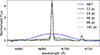 |
Fig. 1. Spectra with normalized continuum around He II 4686 Å for the WN3h star SMC AB 7 (blue) and regions with different apertures from the LVM data, black for the smallest apertures and lighter green for wider ones. |
Only four of our six targets (AB 1, AB 7, AB 9, and AB 12) yield a noticeable imprint of the broad stellar wind line for the 40″ aperture. Beside a dilution due to nebular continuum, these stars also differ in their luminosities (logL/L⊙ ≳ 5.9, Hainich et al. 2015; Shenar et al. 2016) and their stellar neighborhood. In contrast, a target such as AB 10 (logL/L⊙ = 5.56) has a more typical luminosity for the bulk of the known, resolved classical WR population and does not leave any stellar imprint in the 40″ aperture. AB 11 (logL/L⊙ = 5.9) is marginally detected, but likely due to a lack of brighter nearby stars that would further dilute the WR emission lines. Within 40″, AB 11 is clearly the star with the brightest B and V magnitudes. This is not the case for AB 10, which has nearby sources more than an order of magnitude brighter in both bands; for example, AzV 7 (B0).
The blend of the broad He II λ 4686 Å emission line in integrated galaxy spectra is called the “blue WR bump”, mainly present in star-forming galaxies and first detected in the blue compact dwarf galaxy He 2–10 by Allen et al. (1976). The broad He II λ 4686 Å can be generated by both WN and WC stars, but the latter typically also have strong C IV λ 5808 Å emission that give rise to a second bump denoted as “yellow” or ”red”. In the case of the SMC, no WC stars are known, but there is a WO4 star in the wing with significant C IV emission (e.g., Bartzakos et al. 2001; Shenar et al. 2016) that would dominate any yellow bump if it were noticeable within an integrated SMC spectrum (Crowther et al. 2023). In principle, C IV λ 5808 Å emission can also be seen in WN stars (though to a much smaller extent), but it is completely absent in the population of SMC WN3h stars due to the combination of a low carbon abundance and high temperature (and thus high excitation status) in the stellar atmosphere. As such, these stars can at best contribute to a blue bump.
The strength of WR bumps is a popular method of estimating the number of WRs in an unresolved region or galaxy. The LVM data enables us to check popular estimates from López-Sánchez & Esteban (2010) and Crowther et al. (2023) for the blue bump. As we explain in Appendix C, WR populations containing mainly weak-lined WNE stars are a challenge for the approach by López-Sánchez & Esteban (2010). The more specific relation from Crowther et al. (2023) for SMC WNE stars gives a reasonable number on the order of unity if a WR bump is detected, but requires one to make a prior informed decision. Appendix D shows the EW ratios for the extended LVM apertures with respect to the stellar EW, showing that the stellar component is diluted even at 12 pc. At d > 24 pc, the ratio is < 0.025 in all cases, making the WR undetectable.
Overall, we can conclude that the broad emission of any SMC WN3h star is completely diluted (i.e., undetectable) if the flux is integrated over a region with a diameter > 24 pc. This value, which can become even lower in cases of lower WR luminosities or crowding with other bright stars, is considerably smaller than the typical resolution achievable with an IFU in many nearby galaxies (∼50 pc, e.g., in PHANGS-MUSE or DGIS, see Emsellem et al. 2022; Li et al. 2025). Thus, weak-lined WNE stars are easy to hide in integrated light and have been missed in even less resolved galaxy surveys such as CALIFA and MaNGA (Miralles-Caballero et al. 2016; Liang et al. 2020).
3. He II ionizing fluxes
The quantitative spectroscopic analysis with PoWR obtained by Hainich et al. (2015) for SMC AB 1, 9, 10, 11, and 12, and Shenar et al. (2016) for SMC AB 7 provide us with a prediction for the intrinsic log QHeII of the SMC WN3 stars, which we used as a baseline to compare with our nebular line measurements from the LVM data. These models do not include a consistent solution of the wind hydrodynamics for the velocity field (Sander et al. 2017, 2020), which is intrinsically complicated for the weak-lined WN3 stars due to radiatively driven turbulence arising near the wind onset in this regime (Moens et al. 2022). Based on preliminary test calculations, we do not expect drastically effects for the predicted QHeII. For WN2 stars, for which the wind onset is not affected by the same issues, dynamically consistent models can yield higher QHeII of up to 0.8 dex (Sander et al. 2025), but mainly due to a temperature revision in the hydrodynamic analysis, which we do not expect for the WN3 stars.
The lower panels of the figures in Appendix B show the LVM flux-calibrated spectra focusing on the He II 4686 Å line for different apertures. To estimate log QHeII, we used the formula from Kehrig et al. (2015):
![Mathematical equation: $$ \begin{aligned} \text{ Q}(\text{ HeII})=L_{\text{HeII}}/[j(\lambda 4686)/\alpha _{\text{ B}}(\text{ HeII})]\approx L_{\text{ HeII}}/3.66\times 10^{-13}, \end{aligned} $$](/articles/aa/full_html/2025/11/aa57041-25/aa57041-25-eq4.gif) (1)
(1)
where j(λ4686) is the photon energy at 4686 Å and αB(HeII) the recombination rate coefficient assuming case B recombination and Te ∼ 2 × 10⁴ K (Osterbrock & Ferland 2006). We calculated the LHeII with the dereddend LVM spectra, using the same extinction as Hainich et al. (2015), Shenar et al. (2016) and the same reddening law (Gordon et al. 2003, plus a small MW foreground). The resulting log QHeII are shown in Table 1.
Using the ionizing flux ratios from Table 1, we compared the nebular diagnostics with the PoWR analysis results and obtained QHeII, LVM/QHeII, star < 1 for all cases except the apertures of AB 7 with r > 80″. This means that the star alone could produce more than enough photons to ionize the region comprised on the whole fiber apertures. For the AB 7 apertures with r > 80″, the blending with other nearby sources from NGC 395 or SNR E0102-72 in larger apertures could provide an extra source of ionization.
4. Summary and conclusions
The availability of LVM provides a unique opportunity to compare resolved stars with integrated light. Using the region around the He IIλ4686 Å line, we study the imprint of the strongest optical emission line of SMC WN3 stars and of their He II ionizing fluxes in the LVM data, taking different apertures. The broad stellar wind component is always diluted and becomes undetectable in the LVM data when integrating over more than 24 pc in diameter. For the case of AB 1, 9, 10, 11, and 12, the He II ionizing fluxes inferred from detailed atmosphere modeling are at least ∼1.5 times larger than the values measured from the nebular emission. This means that a significant number of ionizing photons from the WN3 targets escape from the immediate environment. In contrast, the larger apertures for AB 7 show an example where the WR alone can produce only up to ∼60% of the observed He II ionizing flux and other, less extreme nearby objects are also contributing to the observed nebular line emission.
While other possible sources of He II ionizing-flux-like massive stellar compact end products such as high-mass X-ray binaries (HMXB, e.g., Plat et al. 2019; Schaerer et al. 2019), intermediate-mass stripped stars (Götberg et al. 2019, 2023), and ultraluminous X-ray (ULX, e.g., Schaerer et al. 2019; Mayya et al. 2023) sources so far could not provide a promising explanation for the significant presence of nebular He II emission in high-z galaxies and metal-poor local galaxies (e.g., Senchyna et al. 2020; Saxena et al. 2020; Wofford et al. 2021, Egorova et al., in prep.), our results show that early-type WN stars with optically thin winds at ≥54 eV are rather easy to “hide”, even when they are at significant distances from larger clusters, despite their strong contribution of He II ionizing photons. While likely not being the exclusive origin of nebular He II, so far current population synthesis models do not reach such an observed WR stage already at SMC metallicities, thereby lacking a potential major contributor. Updated treatments will have major impacts on stellar population predictions and cosmological simulations of galaxy evolution.
Acknowledgments
We thank and E. Tarantino for useful discussions. GGT is supported by the Federal Ministry for Economic Affairs and Climate Action (BMWK) via the Deutsches Zentrum für Luft- und Raumfahrt (DLR) grant 50 OR 2503 (PI Sander). AACS, RRL, and VR acknowledge support by the Deutsche Forschungsgemeinschaft (DFG) in the form of an Emmy Noether Research Group – Project-ID 445674056 (SA4064/1-1, PI Sander). JJ is supported by the DFG under Project-ID 496854903 (SA4064/2-1, PI Sander). ECS is supported by the BMWK via the DLR grant 50 OR 2306 (PI Ramachandran/Sander). This project was co-funded by the European Union (Project 101183150 – OCEANS). EE, KK, and FHL acknowledge funding from the European Research Council’s starting grant ERC StG-101077573(‘ISM-METALS’, PI Kreckel). OE acknowledges funding from the DFG under Project-ID 541068876 (PI Egorov). This work was performed in part at Aspen Center for Physics, which is supported by National Science Foundation grant PHY-2210452. SFS thanks the support by UNAM PASPA – DGAPA, the SECIHTI CBF-2025-I-236 project, and the Spanish Ministry of Science and Innovation (MICINN), project PID2019-107408GB-C43 (ESTALLIDOS). GAB is supported by the ANID Basal project FB210003. Funding for the Sloan Digital Sky Survey V has been provided by the Alfred P. Sloan Foundation, the Heising-Simons Foundation, the National Science Foundation, and the Participating Institutions. SDSS acknowledges support and resources from the Center for High-Performance Computing at the University of Utah. SDSS telescopes are located at Apache Point Observatory, funded by the Astrophysical Research Consortium and operated by New Mexico State University, and at Las Campanas Observatory, operated by the Carnegie Institution for Science. The SDSS web site is www.sdss.org. SDSS is managed by the Astrophysical Research Consortium for the Participating Institutions of the SDSS Collaboration, including the Carnegie Institution for Science, Chilean National Time Allocation Committee (CNTAC) ratified researchers, Caltech, the Gotham Participation Group, Harvard University, Heidelberg University, The Flatiron Institute, The Johns Hopkins University, L’Ecole polytechnique fédérale de Lausanne (EPFL), Leibniz-Institut für Astrophysik Potsdam (AIP), Max-Planck-Institut für Astronomie (MPIA Heidelberg), Max-Planck-Institut für Extraterrestrische Physik (MPE), Nanjing University, National Astronomical Observatories of China (NAOC), New Mexico State University, The Ohio State University, Pennsylvania State University, Smithsonian Astrophysical Observatory, Space Telescope Science Institute (STScI), the Stellar Astrophysics Participation Group, Universidad Nacional Autónoma de México, University of Arizona, University of Colorado Boulder, University of Illinois at Urbana-Champaign, University of Toronto, University of Utah, University of Virginia, Yale University, and Yunnan University.
References
- Allen, D. A., Wright, A. E., & Goss, W. M. 1976, MNRAS, 177, 91 [NASA ADS] [Google Scholar]
- Arellano-Córdova, K. Z., Berg, D. A., Chisholm, J., et al. 2022, ApJ, 940, L23 [CrossRef] [Google Scholar]
- Azzopardi, M., & Breysacher, J. 1979, A&A, 75, 120 [NASA ADS] [Google Scholar]
- Bartzakos, P., Moffat, A. F. J., & Niemela, V. S. 2001, MNRAS, 324, 18 [NASA ADS] [CrossRef] [Google Scholar]
- Boco, L., Mapelli, M., Sander, A. A. C., et al. 2025, A&A, in press https://doi.org/10.1051/0004-6361/202556187 [Google Scholar]
- Bouret, J. C., Lanz, T., Hillier, D. J., et al. 2003, ApJ, 595, 1182 [NASA ADS] [CrossRef] [Google Scholar]
- Breysacher, J., & Westerlund, B. E. 1978, A&A, 67, 261 [NASA ADS] [Google Scholar]
- Calabrò, A., Castellano, M., Zavala, J. A., et al. 2024, ApJ, 975, 245 [CrossRef] [Google Scholar]
- Cameron, A. J., Katz, H., Rey, M. P., & Saxena, A. 2023, MNRAS, 523, 3516 [NASA ADS] [CrossRef] [Google Scholar]
- Conti, P. S. 1975, MSRSL, 9, 193 [NASA ADS] [Google Scholar]
- Crowther, P. A., & Hadfield, L. J. 2006, A&A, 449, 711 [NASA ADS] [CrossRef] [EDP Sciences] [Google Scholar]
- Crowther, P. A., Rate, G., & Bestenlehner, J. M. 2023, MNRAS, 521, 585 [NASA ADS] [CrossRef] [Google Scholar]
- Drory, N., Blanc, G. A., Kreckel, K., et al. 2024, AJ, 168, 198 [NASA ADS] [CrossRef] [Google Scholar]
- Emsellem, E., Schinnerer, E., Santoro, F., et al. 2022, A&A, 659, A191 [NASA ADS] [CrossRef] [EDP Sciences] [Google Scholar]
- Foellmi, C. 2004, A&A, 416, 291 [NASA ADS] [CrossRef] [EDP Sciences] [Google Scholar]
- Foellmi, C., Moffat, A. F. J., & Guerrero, M. A. 2003, MNRAS, 338, 360 [NASA ADS] [CrossRef] [Google Scholar]
- Gordon, K. D., Clayton, G. C., Misselt, K. A., Landolt, A. U., & Wolff, M. J. 2003, ApJ, 594, 279 [NASA ADS] [CrossRef] [Google Scholar]
- Götberg, Y., de Mink, S. E., Groh, J. H., Leitherer, C., & Norman, C. 2019, A&A, 629, A134 [NASA ADS] [CrossRef] [EDP Sciences] [Google Scholar]
- Götberg, Y., Drout, M. R., Ji, A. P., et al. 2023, ApJ, 959, 125 [CrossRef] [Google Scholar]
- Graczyk, D., Pietrzyński, G., Thompson, I. B., et al. 2020, ApJ, 904, 13 [Google Scholar]
- Gräfener, G., & Vink, J. S. 2013, A&A, 560, A6 [NASA ADS] [CrossRef] [EDP Sciences] [Google Scholar]
- Gräfener, G., Koesterke, L., & Hamann, W. R. 2002, A&A, 387, 244 [NASA ADS] [CrossRef] [EDP Sciences] [Google Scholar]
- Guseva, N. G., Izotov, Y. I., & Thuan, T. X. 2000, ApJ, 531, 776 [NASA ADS] [CrossRef] [Google Scholar]
- Hainich, R., Pasemann, D., Todt, H., et al. 2015, A&A, 581, A21 [NASA ADS] [CrossRef] [EDP Sciences] [Google Scholar]
- Hamann, W. R., & Gräfener, G. 2003, A&A, 410, 993 [CrossRef] [EDP Sciences] [Google Scholar]
- Hawcroft, C., Leitherer, C., Aranguré, O., et al. 2025, ApJS, 280, 5 [Google Scholar]
- Herbst, T. M., Bizenberger, P., Blanc, G. A., et al. 2024, AJ, 168, 267 [Google Scholar]
- Kehrig, C., Vílchez, J. M., Pérez-Montero, E., et al. 2015, ApJ, 801, L28 [NASA ADS] [CrossRef] [Google Scholar]
- Kollmeier, J. A., Rix, H.-W., Aerts, C., et al. 2025, AJ, submitted [arXiv:2507.06989] [Google Scholar]
- Leitherer, C., Ekström, S., Meynet, G., et al. 2014, ApJS, 212, 14 [Google Scholar]
- Li, X., Shi, Y., Bian, F., et al. 2025, ArXiv e-prints [arXiv:2501.04943] [Google Scholar]
- Liang, F.-H., Li, C., Li, N., et al. 2020, ApJ, 896, 121 [Google Scholar]
- López-Sánchez, Á. R., & Esteban, C. 2010, A&A, 516, A104 [NASA ADS] [CrossRef] [EDP Sciences] [Google Scholar]
- Martins, F., Hillier, D. J., Bouret, J. C., et al. 2009, A&A, 495, 257 [NASA ADS] [CrossRef] [EDP Sciences] [Google Scholar]
- Massey, P., & Duffy, A. S. 2001, ApJ, 550, 713 [NASA ADS] [CrossRef] [Google Scholar]
- Massey, P., Olsen, K. A. G., & Parker, J. W. 2003, PASP, 115, 1265 [NASA ADS] [CrossRef] [Google Scholar]
- Mayya, Y. D., Plat, A., Gómez-González, V. M. A., et al. 2023, MNRAS, 519, 5492 [NASA ADS] [CrossRef] [Google Scholar]
- Miralles-Caballero, D., Díaz, A. I., López-Sánchez, Á. R., et al. 2016, A&A, 592, A105 [NASA ADS] [CrossRef] [EDP Sciences] [Google Scholar]
- Moens, N., Poniatowski, L. G., Hennicker, L., et al. 2022, A&A, 665, A42 [NASA ADS] [CrossRef] [EDP Sciences] [Google Scholar]
- Morgan, D. H., Vassiliadis, E., & Dopita, M. A. 1991, MNRAS, 251, 51 [Google Scholar]
- Neugent, K. F., Massey, P., & Morrell, N. 2018, ApJ, 863, 181 [NASA ADS] [CrossRef] [Google Scholar]
- Osterbrock, D. E., & Ferland, G. J. 2006, Astrophysics of Gaseous Nebulae and Active Galactic Nuclei (Sausalito, Ca: University Science Books) [Google Scholar]
- Plat, A., Charlot, S., Bruzual, G., et al. 2019, MNRAS, 490, 978 [Google Scholar]
- Pontoppidan, K. M., Barrientes, J., Blome, C., et al. 2022, ApJ, 936, L14 [NASA ADS] [CrossRef] [Google Scholar]
- Ramachandran, V., Hamann, W. R., Oskinova, L. M., et al. 2019, A&A, 625, A104 [NASA ADS] [CrossRef] [EDP Sciences] [Google Scholar]
- Robertson, B. E., Tacchella, S., Johnson, B. D., et al. 2023, Nat. Astron., 7, 611 [NASA ADS] [CrossRef] [Google Scholar]
- Sánchez, S. F., Mejía-Narváez, A., Egorov, O. V., et al. 2025, AJ, 169, 52 [Google Scholar]
- Sander, A. A. C. 2022, ArXiv e-prints [arXiv:2211.05424] [Google Scholar]
- Sander, A., Shenar, T., Hainich, R., et al. 2015, A&A, 577, A13 [NASA ADS] [CrossRef] [EDP Sciences] [Google Scholar]
- Sander, A. A. C., Hamann, W. R., Todt, H., Hainich, R., & Shenar, T. 2017, A&A, 603, A86 [NASA ADS] [CrossRef] [EDP Sciences] [Google Scholar]
- Sander, A. A. C., Vink, J. S., & Hamann, W. R. 2020, MNRAS, 491, 4406 [Google Scholar]
- Sander, A. A. C., Lefever, R. R., Poniatowski, L. G., et al. 2023, A&A, 670, A83 [NASA ADS] [CrossRef] [EDP Sciences] [Google Scholar]
- Sander, A. A. C., Lefever, R. R., Josiek, J., et al. 2025, ArXiv e-prints [arXiv:2508.18410] [Google Scholar]
- Sanduleak, N. 1968, AJ, 73, 246 [Google Scholar]
- Sanduleak, N. 1969, AJ, 74, 877 [NASA ADS] [CrossRef] [Google Scholar]
- Saxena, A., Pentericci, L., Schaerer, D., et al. 2020, MNRAS, 496, 3796 [Google Scholar]
- Schaerer, D. 2003, A&A, 397, 527 [NASA ADS] [CrossRef] [EDP Sciences] [Google Scholar]
- Schaerer, D., Fragos, T., & Izotov, Y. I. 2019, A&A, 622, L10 [NASA ADS] [CrossRef] [EDP Sciences] [Google Scholar]
- Schaerer, D., Marques-Chaves, R., Barrufet, L., et al. 2022, A&A, 665, L4 [NASA ADS] [CrossRef] [EDP Sciences] [Google Scholar]
- Schootemeijer, A., Shenar, T., Langer, N., et al. 2024, A&A, 689, A157 [NASA ADS] [CrossRef] [EDP Sciences] [Google Scholar]
- Schürmann, C., Langer, N., Kramer, J. A., et al. 2024, A&A, 690, A282 [NASA ADS] [CrossRef] [EDP Sciences] [Google Scholar]
- Senchyna, P., Stark, D. P., Vidal-García, A., et al. 2017, MNRAS, 472, 2608 [NASA ADS] [CrossRef] [Google Scholar]
- Senchyna, P., Stark, D. P., Mirocha, J., et al. 2020, MNRAS, 494, 941 [CrossRef] [Google Scholar]
- Shenar, T., Hainich, R., Todt, H., et al. 2016, A&A, 591, A22 [NASA ADS] [CrossRef] [EDP Sciences] [Google Scholar]
- Shenar, T., Hainich, R., Todt, H., et al. 2018, A&A, 616, A103 [NASA ADS] [CrossRef] [EDP Sciences] [Google Scholar]
- Shenar, T., Gilkis, A., Vink, J. S., Sana, H., & Sander, A. 2020, A&A, 634, A79 [NASA ADS] [CrossRef] [EDP Sciences] [Google Scholar]
- Shirazi, M., & Brinchmann, J. 2012, MNRAS, 421, 1043 [NASA ADS] [CrossRef] [Google Scholar]
- Smith, L. F. 1968, MNRAS, 138, 109 [NASA ADS] [CrossRef] [Google Scholar]
- Smith, L. J., Norris, R. P. F., & Crowther, P. A. 2002, MNRAS, 337, 1309 [CrossRef] [Google Scholar]
- Smith, R. C., Points, S. D., Chu, Y. H., et al. 2005, American Astronomical Society Meeting Abstracts, BAAS, 207, 25.07 [Google Scholar]
- Szécsi, D., Langer, N., Yoon, S.-C., et al. 2015, A&A, 581, A15 [NASA ADS] [CrossRef] [EDP Sciences] [Google Scholar]
- Tarantino, E., Bolatto, A. D., Indebetouw, R., et al. 2024, ApJ, 969, 101 [Google Scholar]
- Topping, M. W., Stark, D. P., Senchyna, P., et al. 2025, ApJ, 980, 225 [Google Scholar]
- Trussler, J. A. A., Adams, N. J., Conselice, C. J., et al. 2023, MNRAS, 523, 3423 [NASA ADS] [CrossRef] [Google Scholar]
- Vanbeveren, D., van Bever, J., & De Donder, E. 1997, A&A, 317, 487 [NASA ADS] [Google Scholar]
- Westerlund, B. E., & Smith, L. F. 1964, MNRAS, 128, 311 [NASA ADS] [Google Scholar]
- Wofford, A., Vidal-García, A., Feltre, A., et al. 2021, MNRAS, 500, 2908 [Google Scholar]
- Zickgraf, F. J., Wolf, B., Stahl, O., & Humphreys, R. M. 1989, A&A, 220, 206 [NASA ADS] [Google Scholar]
Appendix A: Observations and atmosphere analyses
The goal of the LVM survey is to map the Milky Way plane, Magellanic Clouds, and a sample of southern, nearby galaxies. The detailed description of the LVM telescope system, science motivation, and technical strategy are given in Herbst et al. (2024), Drory et al. (2024), Sánchez et al. (2025). The LVM instrument is a wide field integral field unit (IFU) telescope built and operated at Las Campanas Observatory (LCO) by SDSS-V (Kollmeier et al. 2025). The LVM IFU has a field of view of 0.5 deg with 1801 hexagonally packed fibers of 35.3″ apertures, with spectral coverage 3600−9800 Å, and spectral resolution R∼4000. All observations of the Magellanic Clouds have a nominal total exposure time of 8100 s, consisting of nine individual 900 s-exposures, dithered following a nine-point grid pattern.
In this work, we focus on the six WN3h SMC stars, whose surrounding nebular emission is covered by the LVM fibers. Figure A.1 shows the location of the targets in the SMC. One more WR system, the WO+O binary AB8 in the SMC Wing, has been identified as a considerable source of QHeII from quantitative spectroscopy (∼5 ⋅ 1047 s−1, Shenar et al. 2016; Ramachandran et al. 2019). However, the LVM has not covered the Wing region yet and we thus focus on the already fully covered sample of early-type WN stars in the SMC in this work.
For all the targets we have plotted the integrated spectra from apertures with 40″, 80″, 160″, 320″, and 600″ diameter. The final spectra were obtained by integrating the spectra from all the fibers that fall inside the given aperture weighted by their effective area (accounting for overlaps by assigning shared pixels fractionally) normalized by the total fiber area. In Figs. A.2 and A.3, we present intensity maps in the He II −4686 Å extracted from the LVM data for the different WN3 stars studied in this work. We further overplot the different apertures we apply for the spectral extraction and comparisons. For some targets, such as AB 9, AB 11, or AB 12 (cf. He II maps in Figs. A.2 and A.3), the largest apertures contain nearby sources also contributing to He II emission, e.g., the sgB[e] LHA 115-S 18 for AB 9 (Zickgraf et al. 1989) or AB 7 falling in the largest aperture around AB 12. These cases illustrate how source blending is an issue in the case of unresolved populations.
For the comparison with the stellar spectra of the WN3 stars, we use optical slit spectroscopy (3700−6830 Å) from Foellmi et al. (2003), Foellmi (2004). The properties of the SMC WR stars were analyzed in Hainich et al. (2015) and Shenar et al. (2016, 2018) using the stellar atmosphere code PoWR (Gräfener et al. 2002; Hamann & Gräfener 2003; Sander et al. 2015).
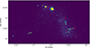 |
Fig. A.1. Position of the WN stars studied in this work, using the identifiers by their number as SMC AB#. The background image shows the O III nebular emission from MCELS (Smith et al. 2005). |
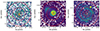 |
Fig. A.2. The He II −4686 Å intensity map centered at SMC AB1 (left), SMC AB7 (center), and SMC AB9 (right) with the corresponding apertures in blue of 40″ (12 pc), 80″ (24 pc), 160″ (48 pc), 320″ (96 pc) and 600″ (181 pc) of diameter. |
Appendix B: The He II −4686 Å line
Normalized and flux calibrated spectra around the He II −4686 Å line is shown in Figures. B.1 – B.6, revealing notable differences between the targets:
-
SMC AB1: The small aperture of 40″ still shows some stellar He II contribution. We have fitted a gaussian distribution and detected faint present nebular emission, as seen in the lower panel of Fig. B.1. The aperture of 320″ shows very weak and narrow He II nebular emission, while it is almost non-detectable for the 600″ aperture.
-
SMC AB7: For the smaller aperture of 40″, the broad stellar component can still be detected, along with a strong nebular emission on top. For higher apertures only the narrow nebular emission is present. (Tarantino et al. 2024) has modeled the surrounding ISM gas for Spitzer IRS data using parameters from Shenar et al. (2016), reproducing several ionizing lines in the far infrared region.
-
SMC AB9: Similar to AB7, but weaker nebular emission.
-
SMC AB10: The nebular emission is very strong already in the 40″ aperture, while the broad stellar contribution is completely hidden.
-
SMC AB11: Very faint to no emission is detected.
-
SMC AB12: Faint stellar stellar emission in the 40″ aperture. The nebular emission increases with wider apertures.
As only the area under the curves is of interest for this work, we did not perform a radial velocity correction for the LVM data.
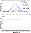 |
Fig. B.1. The He II −4686 Å line profile for the SMC AB1 region. Upper panel: The normalized flux for the He II −4686 Å line profile for the SMC AB1 target, in blue for the data of the star (from Foellmi et al. 2003), black for the smallest fiber aperture of LVM (40″), lighter gray for wider apertures. Lower panel: The calibrated flux for the He II −4686 Å line profile for the SMC AB1 nebular region, black for the smallest fiber aperture of LVM (40″), lighter gray for wider apertures. In light blue we show the regions selected of the He II that contribute to the nebular component. |
Appendix C: Detecting the blue WR bump
To get an estimate of the total number of WR stars in an integrated population showing WR bumps, López-Sánchez & Esteban (2010) created a widely used formula based on the line luminosities provided by Crowther & Hadfield (2006) with a linear interpolation between the data for Z⊙ and Z⊙/50. However, these relations attribute the blue and red bumps only to late-type WN (WNL) and early-type WC stars and thus a WR population with mainly early-type WNE stars like in the SMC would be misinterpreted. In fact, any application of the López-Sánchez & Esteban (2010) on the LVM SMC WNE data would yield numbers way below unity. More recently, Crowther et al. (2023) presented detailed line luminosities for a large sample of WR stars from the Milky Way, the LMC and the SMC. For the summarized luminosity of early-type WN stars, Crowther et al. (2023) calculates LWN2-5(He II λ4686) at the SMC metallicity to be 1.7 × 1035 erg s−1 (see their Table 2).
Table C1 shows the estimated number of WN stars in our LVM regions using the luminosity values from López-Sánchez & Esteban (2010), Crowther & Hadfield (2006), Crowther et al. (2023) compared to our LVM LHeII, VLM calculations (using the broad stellar component in the LVM flux calibrated spectra). We have used the apertures with a signal being 5% greater than the noise, which corresponds to a diameter of ≤24 pc, while the for wider apertures the wide stellar component was completely not detectable.
Target, the corresponding region and the estimated number of WN stars for 1/5 Z⊙.
Appendix D: EW ratios with respect to the distance
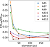 |
Fig. D.1. Ratio of Equivalent Widths (EW) of the extended stellar emission component of He II 4686 Å seen by LVM to the intrinsic stellar EW. |
All Tables
Target, the corresponding region and the estimated number of WN stars for 1/5 Z⊙.
All Figures
|
Fig. 1. Spectra with normalized continuum around He II 4686 Å for the WN3h star SMC AB 7 (blue) and regions with different apertures from the LVM data, black for the smallest apertures and lighter green for wider ones. |
| In the text | |
|
Fig. A.1. Position of the WN stars studied in this work, using the identifiers by their number as SMC AB#. The background image shows the O III nebular emission from MCELS (Smith et al. 2005). |
| In the text | |
|
Fig. A.2. The He II −4686 Å intensity map centered at SMC AB1 (left), SMC AB7 (center), and SMC AB9 (right) with the corresponding apertures in blue of 40″ (12 pc), 80″ (24 pc), 160″ (48 pc), 320″ (96 pc) and 600″ (181 pc) of diameter. |
| In the text | |
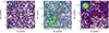 |
Fig. A.3. Same as Fig. A.2 but for SMC AB10 (left), SMC AB11 (center), and SMC AB12 (right). |
| In the text | |
|
Fig. B.1. The He II −4686 Å line profile for the SMC AB1 region. Upper panel: The normalized flux for the He II −4686 Å line profile for the SMC AB1 target, in blue for the data of the star (from Foellmi et al. 2003), black for the smallest fiber aperture of LVM (40″), lighter gray for wider apertures. Lower panel: The calibrated flux for the He II −4686 Å line profile for the SMC AB1 nebular region, black for the smallest fiber aperture of LVM (40″), lighter gray for wider apertures. In light blue we show the regions selected of the He II that contribute to the nebular component. |
| In the text | |
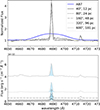 |
Fig. B.2. Same as Fig. B.1 but for SMC AB7. |
| In the text | |
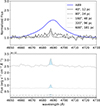 |
Fig. B.3. Same as Fig. B.1 but for SMC AB9. |
| In the text | |
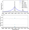 |
Fig. B.4. Same as Fig. B.1 but for SMC AB10. |
| In the text | |
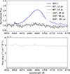 |
Fig. B.5. Same as Fig. B.1 but for SMC AB11. |
| In the text | |
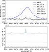 |
Fig. B.6. Same as Fig. B.1 but for SMC AB12. |
| In the text | |
|
Fig. D.1. Ratio of Equivalent Widths (EW) of the extended stellar emission component of He II 4686 Å seen by LVM to the intrinsic stellar EW. |
| In the text | |
Current usage metrics show cumulative count of Article Views (full-text article views including HTML views, PDF and ePub downloads, according to the available data) and Abstracts Views on Vision4Press platform.
Data correspond to usage on the plateform after 2015. The current usage metrics is available 48-96 hours after online publication and is updated daily on week days.
Initial download of the metrics may take a while.