| Issue |
A&A
Volume 703, November 2025
|
|
|---|---|---|
| Article Number | A146 | |
| Number of page(s) | 6 | |
| Section | The Sun and the Heliosphere | |
| DOI | https://doi.org/10.1051/0004-6361/202557055 | |
| Published online | 14 November 2025 | |
Helicities of the polarity-inversion line and solar eruptivity
1
Physics Department, University of Ioannina, Ioannina GR-45110, Greece
2
University of Graz, Institute of Physics, Universitätsplatz 5, 8010 Graz, Austria
⋆ Corresponding author: This email address is being protected from spambots. You need JavaScript enabled to view it.
Received:
1
September
2025
Accepted:
23
September
2025
Abstract
Aims. We examine the relation between solar eruptivity and the relative helicity that is contained around the polarity-inversion line (PIL) of the magnetic field, along with its current-carrying component.
Methods. To this end, we analysed the evolution of the PIL helicities in a sample of ∼40 solar active regions that exhibited more than 200 flares of class M or higher. We computed the PIL helicities with the help of the relative field line helicity, the recently developed proxy for the density of relative helicity, following the extrapolation of the 3D coronal magnetic field with a non-linear force-free method.
Results. The relative helicity of the PIL decreases significantly on average by more than 10% during stronger eruptive flares (M5.0 class and above), while smaller changes are observed for confined and/or weaker flares. The PIL current-carrying helicity shows higher-magnitude decreases in strong and weak flares and reaches an average of 20% of changes during the stronger eruptive flares. Notably, the PIL current-carrying helicity differs most between eruptive and confined flares, which indicates its strong potential as a diagnostic of solar eruptivity. We discuss the implications of these findings for solar flare forecasting.
Key words: magnetohydrodynamics (MHD) / methods: numerical / Sun: activity / Sun: fundamental parameters / Sun: magnetic fields
© The Authors 2025
 Open Access article, published by EDP Sciences, under the terms of the Creative Commons Attribution License (https://creativecommons.org/licenses/by/4.0), which permits unrestricted use, distribution, and reproduction in any medium, provided the original work is properly cited.
This article is published in open access under the Subscribe to Open model. This email address is being protected from spambots. You need JavaScript enabled to view it. to support open access publication.
1. Introduction
Magnetic helicity is a geometrical quantity that describes the complexity of a magnetic field because it is related to the twist and writhe of individual magnetic field lines and to the intertwining of pairs of field lines. It is conserved in ideal magnetohydrodynamics (MHD; Woltjer 1958) and is therefore important in studies of magnetised systems. The appropriate mathematical form of helicity in solar conditions, where magnetic flux is exchanged between the solar interior and atmosphere, is relative helicity (Berger & Field 1984). This is defined by
 (1)
(1)
where B stands for the 3D magnetic field in the coronal volume of interest V, Bp for a suitable reference magnetic field, and A and Ap are the respective vector potentials. We refer to Hr in the following simply as helicity, or volume helicity.
The connection between helicity and solar eruptivity was recognized immediately when helicity began to be used in studies of observed active regions (ARs). It was then found that eruptive flares, that is, flares that are accompanied by coronal mass ejections (CMEs), have a higher helicity statistically than ARs that exhibit confined flares (Nindos & Andrews 2004). Nindos & Andrews (2004) also identified a helicity threshold of 1.5 × 1042 Mx2 above which ARs tend to produce CMEs. This was later confirmed by Tziotziou et al. (2012, 2 × 1042 Mx2) and Liokati et al. (2023, 9 × 1041 Mx2). More recently, Thalmann et al. (2025) found favorable conditions for strong flaring (GOES class M1.0 or higher) when the helicity exceeds 1 × 1042 Mx2 (see their Fig. 8a). This supports the earlier statistical studies.
A quite successful helicity-derived eruptivity indicator is the so-called helicity eruptivity index (HEI; Pariat et al. 2017). This is the ratio |Hj|/|Hr|, where Hj = ∫V(A − Ap)⋅(B − Bp) dV is the current-carrying helicity, which is one of the two components in the unique decomposition of helicity, the other being the volume-threading helicity (Berger 1999; Linan et al. 2018). The dedicated numerical experiment by Pariat et al. (2023) showed that the values of HEI during the pre-eruptive phase are high for eruptive cases, in which the unstable flux rope is later expelled from the simulation volume. In particular, their eruptive simulation setup involved an (overlying) arcade field oriented anti-parallel to the direction of the upper part of the emerging twisted flux rope. In contrast, for simulation setups that involved a quasi-parallel arcade field, the pre-eruption values of the HEI remained low. This agrees with the simulation-based study by Rice & Yeates (2022), who showed that the HEI only has a weak predictive skill and is lower and not higher before eruptions when the overlying background magnetic field has the same direction as the arcade. The authors concluded that a whole class of solar eruptions therefore cannot be predicted by a high HEI. Nevertheless, the recent statistical study by Thalmann et al. (2025), based on data-constrained coronal magnetic field modelling of 40 solar ARs, revealed that the corona shows a higher overall value of the HEI before eruptive flares than the characteristic non-eruptive pre-flare corona. The highest values of the HEI, however, were found not just before the onset of CMEs, but persisted over extended time periods. An exceeded suggested critical value therefore cannot serve as an indicator for near-in-time upcoming eruptive activity.
With the routine measurements of the magnetic field with the Solar Dynamics Observatory (SDO; Pesnell et al. 2012) in recent years, the interest in helicity has expanded to include the calculation of the changes it undergoes during solar flares. In a sample of 21 X-class flares, Liu et al. (2023) found that when a flare is associated with a CME, it is accompanied by strong decreases in helicity (∼17% of the pre-flare values on average), while this is not the case for confined flares. This was further quantified by Wang et al. (2023) for 47 flares of GOES class M4.0 or higher, in which the helicity dropped by ∼15% in the CME-associated flares and by ∼1% in the confined flares. Similar results were obtained by Thalmann et al. (2025) based on a much more extended flare sample (220 flares of GOES class M1 or higher). Furthermore, for the subset of major flares (GOES class M5 or higher), they found characteristic decreases in the helicity of ∼12% and ∼1% for CME-associated and confined (CME-less) events, respectively.
Two additional helicity-related quantities that have recently attracted attention are the relative helicity that is contained around the magnetic polarity-inversion line (PIL; Moraitis et al. 2024a) and its corresponding current-carrying component (Moraitis et al. 2024b). Moraitis et al. (2024a) and Moraitis et al. (2024b) demonstrated that the evolution of the PIL helicities follows that of the volume helicities in general and that the PIL helicities change more strongly as a result of the flares than the volume helicities. Moraitis et al. (2024a) quantified this difference to a decrease by ∼7% for the PIL relative helicity on average and to a decrease of only ∼1% for the volume helicity, based on their study of 22 CME-associated and CME-less flares with a class higher than M1.0.
The main aim of this work is to examine the statistical distributions of the changes in the two PIL helicities during solar flares in the large flare sample of Thalmann et al. (2025), which contains a good balance of CME-associated and confined flares, to expand on the works of Moraitis et al. (2024a) and Thalmann et al. (2025). In Sect. 2 we describe the main characteristics of the flare sample we used. In Sect. 3 we define all quantities of interest and the method with which we computed them from the observational data. In Sect. 4 we present the results, and in Sect. 5 we summarize and discuss our results.
2. Flare sample
We studied the PIL helicities in the same flare sample as Thalmann et al. (2025). We repeat its basic characteristics below. The flares we analysed have a GOES class M1 or higher, and they correspond to 36 different ARs. These are most of the ARs observed with the Helioseismic and Magnetic Imager (HMI; Scherrer et al. 2012) on board SDO during the rising phase of Solar Cycle 24, which lasted from February 2011 to September 2017.
The whole sample consists of 220 M- and X-class flares, of which 116 are confined flares and 104 are associated with a CME. It is denoted SM1+ and it can be split into two subsets: the weaker flares, and the major flares. The weaker flares are up to class M4.9 and are 172 in total, of which 102 are confined and 70 are associated with a CME. The major flares (sample Smajor) are 48 flares with a class higher than M5.0, of which 14 are confined flares, and 34 are associated with a CME. They can also be split into 26 M-class flares (8 confined flares and 18 that are associated with a CME, and 22 X-class flares (6 confined, 16 associated with a CME). The number of flares we quote here comes from Table 1 of Thalmann et al. (2025), and we subtracted the 11 flares that were associated with a flare-related change in the sign of helicity and therefore had unreliable pre-flare values. More details can be found in Thalmann et al. (2025). From all the information of the original flare sample, we only used the start and end times of the flares for our analysis, tstart and tend, their strength, and whether a flare was associated with a CME.
3. Method
In order to compute the quantities of interest, we modelled the 3D magnetic field in the coronal volume for each target AR around the time of the flares, starting from the observed magnetograms. We used the non-linear force-free (NLFF) method of Wiegelmann et al. (2012) to do this, as implemented and described by Thalmann et al. (2025). We recall that the NLFF modelling involves solving the force-free boundary value problem on an initially coarse grid with boundaries specified by a potential field solution (computed from the observed vertical magnetic field component). The solution of the coarse grid is then sampled to the final NLFF model grid and serves as a start equilibrium (hence boundary condition). By design, the optimisation method weights the initial equilibrium so that its effect drops in form of a cosine-profile towards the lateral and top boundaries (Wiegelmann 2004). The exact boundary conditions therefore affect the final NLFF model little, if at all. We also emphasise that the NLFF reconstruction uses an enhanced weighting for the volume-integrated divergence so that the solenoidal quality of the solutions is sufficient, which is necessary for computing the helicity (Valori et al. 2016). The 3D NLFF models are employed based on a variable time cadence, typically 12 min around flare peak times and 1 hr otherwise. Each of the employed NLFF solutions was verified, and unphysical and low-quality solutions were identified and excluded from the further analysis.
For all qualifying 3D NLFF models, we computed the reference potential field (Bp) and the vector potentials of the two fields (A and Ap), following the method of Moraitis et al. (2014). We recall that the two vector potentials are taken in the DeVore (2000) gauge and that Ap additionally satisfies the Coulomb gauge. These four vector fields allow us to calculate the free energy, Ej = ∫V(B − Bp)2 dV/(8π), the volume relative helicity, Hr, and the volume current-carrying helicity, Hj.
We also computed the relative field line helicity (FLH; hr; Yeates & Page 2018; Moraitis et al. 2019) and its current-carrying component (hj; Moraitis et al. 2024b). These FLHs can be considered as the densities of the respective helicities and are gauge-dependent in general. The choice of the DeVore gauge facilitates computations, and, as shown by Moraitis et al. (2024a), produces results to within 10% from other gauge choices. The computation of the FLHs requires integrating the vector potentials along the magnetic field lines of B and Bp. The field lines were integrated with a modification of the code qfactor (Liu et al. 2016), which can be found online1.
The next step was to identify the PIL for each target AR and time of interest, which we did with the method of Schrijver (2007) and with the same parameters as in Moraitis et al. (2024a): a magnetic field threshold of 150 G, and a dilation window of 3x3 pixels. The convolution of the PIL with an area-normalized Gaussian with a full width at half maximum of 9″resulted in a 2D mask WPIL at the lower model boundary (z = 0). With the help of the FLHs, we computed the relative helicity that is contained around the PIL from
 (2)
(2)
and its respective current-carrying component from
 (3)
(3)
where dΦ stands for the element of magnetic flux. We refer in the following to these helicities as the PIL relative helicity and the PIL current-carrying helicity, respectively.
The time cadence is variable, and we therefore interpolated all quantities of interest first to a constant-cadence timeseries of 12 min. Then, the interpolated time arrays were smoothed with a two-hour smoothing window so that sharp changes were eliminated. The effect of these processes is shown in Fig. 2 of Thalmann et al. (2025). Finally, we estimated the flare-related changes of the various quantities. For a quantity Q, we defined its relative change during a flare as
 (4)
(4)
where Qpre is the mean pre-flare value of Q in the hour prior to the flare start time, that is, in the interval tstart − 60 min ≤ t ≤ tstart, and similarly, Qpost is its mean post-flare value in the hour after the flare end time, that is, in the interval tend ≤ t ≤ tend + 60 min. Qpre and Qpost were both considered with their respective sign. The quantity ηQ is identical to the η parameter of Thalmann et al. (2025) and similar in scope to the relative change Δf of Moraitis et al. (2024a). A negative (positive) value of ηQ denotes a decrease (increase) in Q during that flare.
4. Results
With the method described above, we computed the various quantities and focused on their flare-related changes in either of the flare samples of interest. We examined three quantities that are known for their sensitivity with respect to solar eruptivity: the free energy, the volume relative helicity, and the volume current-carrying helicity. These were also examined by Thalmann et al. (2025) and were used to interpret our results. Our main interest was the relative helicity and current-carrying helicity of the PIL.
For each of these five quantities, we computed the distributions of their flare-related changes (ηQ). For each distribution, we computed the mean and standard deviation and also its median value and interquartile range (IQR), that is, the range between the 75th and 25th percentiles. The latter two are insensitive to outlier values that affect the mean and standard deviation, and we therefore used them as independent measures of the central tendency and dispersion for each distribution. Nevertheless, we limit the level of outlier values to ±100% in the following, that is, we omit any flare-related changes outside these limits because the values were extreme in some cases. This occurred when the mean pre-flare values are very low or when the PIL identification resulted in very few points.
The mean value for the flare-related change in free energy for the sample of flares Smajor is ⟨ηEj⟩= − 10.3%±1.5%. For the CME-associated flares alone, it is −12.2%±1.8%, and it is −5.7%±2.1% for confined flares. These values are very close to the respective values −13.3%±5.0% and −5.2%±2.5% of Thalmann et al. (2025). We attribute the small differences to the different computational methods used in deriving the basic quantities. The median values for free energy are all very close to the respective means, −11.4%, −13.7%, and −6.5%, and the latter are therefore to be trusted, also because their IQRs are small, 16.5%, 16.3%, and 8.8%.
The mean value for the flare-related change in the volume relative helicity is ⟨ηHr⟩= − 9.8%±2.1% for the whole Smajor sample, −13.0%±2.8% for the CME-associated flares, and −2.3%±1.3% for the confined flares. The latter two are very close to those of Thalmann et al. (2025), −11.5%±5.0% and −1.4%±1.9%, respectively. As an example of the effect of limiting the outliers to the interval [ − 100%,100%], we mention that the mean ⟨ηHr⟩ for the CME-associated flares would have been much higher if we had not restricted the outliers, namely −21.2%±8.6%, although the medians would be similar, −12.0% in the unrestricted and −11.8% in the restricted case. By applying the limiting, however, we obtained a mean change similar to the median, where the IQR is additionally 16.7%. The mean and median values of the confined flares disagree because the median is −4.6% with an IQR of 8.1%. For all major flares, the median and IQR of the distribution of ηHr are −9.4% and 13.1%, respectively.
The volume current-carrying helicity has strong flare-related changes overall. For all the major flares, the change is ⟨ηHj⟩= − 16.6%±2.6%, for the CME-associated flares, the change is −19.4%±3.3%, and for the confined flares, the change −9.8%±3.5%. The respective median values are close to the means, −14.7%, −21.3%, and −11.3%, and the IQRs are higher than in the previous two quantities, namely 23.7%, 24.8%, and 11.9%. The numbers for the CME-associated and confined flares agree very well with those of Thalmann et al. (2025), which are −18.2%±6.5% and −9.0%±4.1%, respectively.
We now focus on the two PIL helicities, starting with the PIL relative helicity, given by Eq. (2). The distribution of the ηHr, PIL for all the flares of the sample Smajor is shown in the left panel of Fig. 1, divided into CME-associated flares (with red colour), and confined flares (with blue). The mean flare-related change for Hr, PIL is ⟨ηHr, PIL⟩= − 11.8%±3.2% for CME-associated flares and −2.9%±10.2% for confined flares. The median values of the distributions agree with the means; they are −11.4% and −2.8%, respectively, while their IQRs are 18.4% and 28.8%. For CME-associated and confined flares together, the respective mean η value is in between the two, −9.2%±3.7%, with a median of −10.6% and IQR 22.7%. The changes in the PIL relative helicity are similar to those of the volume relative helicity in all cases.
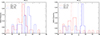 |
Fig. 1. Histograms of the relative change during the flares (η, in percent of the pre-flare values) of the PIL relative helicity (left) and of its current-carrying component (right). CME-associated flares are depicted in red, and confined flares are shown in blue. The vertical dotted lines represent the mean values of the respective distributions, and the dashed lines show the median values. |
The PIL current-carrying helicity, which is given by Eq. (3), is shown in the right panel of Fig. 1. We find mean flare-related changes ⟨ηHj, PIL⟩= − 12.7%±5.3% for all the major flares, −17.5%±4.7% for the CME-associated ones, and −1.4%±13.7% for the confined flares. The respective median values are relatively close to the means for all, and the CME-associated flares, −17.6% and −21.6%, but differ for the confined flares, where the median is 6.6%. Moreover, their IQRs are high, 37.5%, 22.4%, and 51.9%, respectively. The high IQR values indicate that the corresponding distributions are quite broad, that is, they have many outlier values. The comparison of the mean and median values indicates that the number of outlier changes of Hj, PIL is larger for the confined flares. The changes in the PIL current-carrying helicity are similar to those of the volume Hj for the CME-associated flares (−17.5% and −19.4%, respectively), but differ strongly for the confined flares (−1.4% and −9.8%, respectively).
All these results are summarised in Table 1. For completeness, we list in the lower part of Table 1 the mean and median values of all distributions for the sample SM1+, that is, for all examined flares. As expected, all values are lower than their corresponding upper-part values for the sample Smajor. This implies that the changes during the weaker flares are minimal. The highest flare-related decreases are also again found in the two current-carrying helicities, volume and PIL, which both exceed 7.5%.
Characteristics (mean, median, and IQR) of the relative flare-related change distributions (ηQ, in units of percents), divided horizontally into CME-associated, confined, and all flares, and divided vertically into major and all flares.
We also note that the relative change in Hr, PIL for all the flares, which has a mean value of −3.8%±1.6%, a median of −4.7%, and an IQR 17.4%, is close to the results of Moraitis et al. (2024a), who reported Δf ∼ −6.5%. The two works are not directly comparable, however, because the pre- and post-flare states were defined differently. They are determined with respect to tstart and tend in this work, but Moraitis et al. (2024a) used the peak of the flares to define the pre- and post-flare states.
Morover, these authors speculated that the relative change in Hr, PIL would have been stronger when CME-associated flares were considered alone, and this is indeed the case for the sample of major flares. For the sample SM1+, however, the differences between CME-associated and confined flares are much smaller.
Finally, the five examined quantities exhibit flare-related decreases in ∼67% of all the CME-associated flares, which increases to ∼88% when the major flares are considered alone. The lowest values are found in the PIL relative helicity. The respective numbers for the confined flares are much smaller in all but the free energy and the volume current-carrying helicity, where they are comparable with the CME-associated case.
We also examined the simultaneous decreases of all possible pairs of quantities. The highest value is found for the pair Ej–Hj in CME-associated and confined flares and is independent of whether a flare is a major or a weak flare. For the sample SM1+, we find a simultaneous decrease in ∼60% of the CME-associated flares and in ∼57% of the confined flares, while for Smajor, this increases to ∼85% and ∼79%, respectively. These numbers are comparable to those reported by Thalmann et al. (2025).
5. Discussion
We examined the statistical distributions of the flare-induced changes of free energy and of various helicity-related quantities in a large sample of solar flares. A high-quality NLFF reconstruction of the coronal magnetic field was used in order to compute the relative and current-carrying helicities in the entire (flare-relevant) model volume, and associated with the flare-related PIL.
Our main results are listed below.
-
All quantities we examined decrease on average during solar flares. When we distinguished between weaker and major flares, we found that the flare-related changes are much stronger in the latter. As an example, the mean change in Hr during all flares is −3.3%, and for the major flares it is −9.8%.
-
The changes resulting from CME-associated flares are always much stronger than in confined flares, especially for major flares.
-
We confirmed the previous findings by Thalmann et al. (2025) about the changes in the free energy and of volume relative and current-carrying helicities.
-
The changes in the PIL relative helicity are comparable to those of the respective volume helicity in all cases. This differs from what was reported by Moraitis et al. (2024a) for a less well-balanced flare sample. The level of Hr, PIL changes when we consider all flares is similar to that work, however.
-
The two current-carrying helicities, volume and PIL, show the most pronounced response to flares. The latter especially shows the largest differences between CME-associated and confined major flares, −17.5% compared to −1.4%. Even when the weaker flares are included, the numbers for Hj, PIL still stand out.
The last result can be understood theoretically because the current-carrying field is mostly related to coronal flux ropes (e.g., Guo et al. 2017). In CME-associated flares, where the flux rope is expelled, the current-carrying helicity decreases as it is carried away with the flux rope, while in confined flares, it remains largely conserved. This behaviour seems to be captured better by the PIL current-carrying helicity than by the volume helicity.
Our results reaffirm the importance of the PIL in understanding the creation of solar flares. In addition to the enhanced magnetic flux and electrical currents along the PIL during flares (Schrijver 2007; Janvier et al. 2014), this region also exhibits a pronounced buildup of current-carrying helicity, which is naturally depicted in the PIL current-carrying helicity. The changes in this quantity thus reflect the changes in the coronal field that is rooted in the PIL during solar flares.
The similar variations in PIL and volume relative helicities may raise the question whether the regions of the AR away from the PIL are just as important as the PIL itself. To examine this possibility, we compute in Appendix A the distributions of the flare-related changes in relative and current-carrying helicities that are contained in the region outside of the PIL. The analysis there shows that although the average flare-related changes in the relative helicity inside and outside of the PIL (for the major CME-associated flares) are comparable, the individual values are much more spread outside of the PIL, and more values are positive in that case. For the current-carrying helicity, the average values are lower, but still negative outside of the PIL, and the distribution is again much broader than for the PIL. The wider spread of these two distributions might be attributed to the much wider range of field line shapes in the region outside of the PIL. For the confined flares, the two helicities outside of the PIL are concentrated more strongly around 0 than the respective PIL cases. We conclude that although the general trends are similar in the PIL and outside it, regions away from the PIL play a smaller role than the PIL itself. This effect is more pronounced for the current-carrying helicity than for the relative helicity.
The PIL helicities have the largest uncertainties of all examined quantities. This is expected because of the computational method we used, especially the PIL identification algorithm, and was already noted by Moraitis et al. (2024b). Even when we consider the least favourable limits of Table 1 for the PIL current-carrying helicity however, we find that decreases by ≳13% of this quantity indicate a major CME-associated flare. The criterion ηHj, PIL ≲ −13% might thus be used in attempts to forecast solar activity that affects space weather imminently. Other factors have to be taken into account when the possible impact on Earth is considered, such as the location of the AR on the solar disc, or the relative orientation between the interplanetary and Earth magnetic fields (e.g., Dumbović et al. 2021; Thalmann et al. 2023). Moreover, a complete study at times without flaring should be carried out as well to eliminate the possibility of false positives of the method. Although they were not addressed in this study, these topics might be examined in a future investigation.
A drawback of using the PIL current-carrying helicity in a forecasting method is the computational effort it requires. This mostly stems from the extrapolation of the magnetic field to the coronal volume (for recent advances see, e.g., Jarolim et al. 2023). Potential ways to accelerate the computation of this PIL helicity will be pursued in future work.
Acknowledgments
The authors thank the referee for providing constructive comments. KM has received funding from the ERC Whole Sun Synergy grant No 810218. JT was funded in part by the Austrian Science Fund (FWF) grants 10.55776/P31413 and 10.55776/PAT7894023. JT acknowledges the High Performance Computing (HPC) center of the University of Graz for providing computational resources and technical support. NASA’s SDO satellite and the HMI instrument were joint efforts by many teams and individuals, whose efforts are greatly appreciated.
References
- Berger, M. A. 1999, Plasma Phys. Controlled Fus., 41, B167 [Google Scholar]
- Berger, M. A., & Field, G. B. 1984, J. Fluid. Mech., 147, 133 [Google Scholar]
- DeVore, C. R. 2000, ApJ, 539, 944 [Google Scholar]
- Dumbović, M., Veronig, A. M., Podladchikova, T., et al. 2021, A&A, 652, A159 [NASA ADS] [CrossRef] [EDP Sciences] [Google Scholar]
- Guo, Y., Pariat, E., Valori, G., et al. 2017, ApJ, 840, 40 [NASA ADS] [CrossRef] [Google Scholar]
- Janvier, M., Aulanier, G., Bommier, V., et al. 2014, ApJ, 788, 60 [Google Scholar]
- Jarolim, R., Thalmann, J. K., Veronig, A. M., & Podladchikova, T. 2023, Nat. Astron., 7, 1171 [NASA ADS] [CrossRef] [Google Scholar]
- Linan, L., Pariat, É., Moraitis, K., Valori, G., & Leake, J. 2018, ApJ, 865, 52 [NASA ADS] [CrossRef] [Google Scholar]
- Liokati, E., Nindos, A., & Georgoulis, M. K. 2023, A&A, 672, A38 [NASA ADS] [CrossRef] [EDP Sciences] [Google Scholar]
- Liu, R., Kliem, B., Titov, V. S., et al. 2016, ApJ, 818, 148 [Google Scholar]
- Liu, Y., Welsch, B. T., Valori, G., et al. 2023, ApJ, 942, 27 [NASA ADS] [CrossRef] [Google Scholar]
- Moraitis, K., Tziotziou, K., Georgoulis, M. K., & Archontis, V. 2014, Sol. Phys., 289, 4453 [Google Scholar]
- Moraitis, K., Pariat, E., Valori, G., & Dalmasse, K. 2019, A&A, 624, A51 [NASA ADS] [CrossRef] [EDP Sciences] [Google Scholar]
- Moraitis, K., Patsourakos, S., Nindos, A., Thalmann, J. K., & Pariat, É. 2024a, A&A, 683, A87 [NASA ADS] [CrossRef] [EDP Sciences] [Google Scholar]
- Moraitis, K., Archontis, V., & Chouliaras, G. 2024b, A&A, 690, A181 [NASA ADS] [CrossRef] [EDP Sciences] [Google Scholar]
- Nindos, A., & Andrews, M. D. 2004, ApJ, 616, L175 [NASA ADS] [CrossRef] [Google Scholar]
- Pariat, E., Leake, J. E., Valori, G., et al. 2017, A&A, 601, A125 [CrossRef] [EDP Sciences] [Google Scholar]
- Pariat, E., Wyper, P. F., & Linan, L. 2023, A&A, 669, A33 [NASA ADS] [CrossRef] [EDP Sciences] [Google Scholar]
- Pesnell, W. D., Thompson, B. J., & Chamberlin, P. C. 2012, Sol. Phys., 275, 3 [Google Scholar]
- Rice, O. E. K., & Yeates, A. R. 2022, Front. Astron. Space Sci., 9, 849135 [NASA ADS] [CrossRef] [Google Scholar]
- Scherrer, P. H., Schou, J., Bush, R. I., et al. 2012, Sol. Phys., 275, 207 [Google Scholar]
- Schrijver, C. J. 2007, ApJ, 655, L117 [Google Scholar]
- Thalmann, J. K., Dumbović, M., Dissauer, K., et al. 2023, A&A, 669, A72 [NASA ADS] [CrossRef] [EDP Sciences] [Google Scholar]
- Thalmann, J. K., Gupta, M., Veronig, A. M., & Liu, Y. 2025, A&A, 695, A66 [NASA ADS] [CrossRef] [EDP Sciences] [Google Scholar]
- Tziotziou, K., Georgoulis, M. K., & Raouafi, N.-E. 2012, ApJ, 759, L4 [NASA ADS] [CrossRef] [Google Scholar]
- Valori, G., Pariat, É., Anfinogentov, S., et al. 2016, Space Sci. Rev., 201, 147 [Google Scholar]
- Wang, Q., Zhang, M., Yang, S., Yang, X., & Zhu, X. 2023, Res. Astron. Astrophys., 23, 095025 [CrossRef] [Google Scholar]
- Wiegelmann, T. 2004, Sol. Phys., 219, 87 [NASA ADS] [CrossRef] [Google Scholar]
- Wiegelmann, T., Thalmann, J. K., Inhester, B., et al. 2012, Sol. Phys., 281, 37 [NASA ADS] [Google Scholar]
- Woltjer, L. 1958, Proc. Nat. Acad. Sci., 44, 489 [Google Scholar]
- Yeates, A. R., & Page, M. H. 2018, J. Plasma Phys., 84, 775840602 [Google Scholar]
Appendix A: Helicities in the region outside of the PIL
This Appendix addresses the question of how important is the (relative and current-carrying) helicity content in the region outside of the PIL. We start by defining a complementary to WPIL mask,  , as:
, as:
 (A.1)
(A.1)
This mask selects all field lines on the photosphere other than the PIL. With the help of  we can define the relative helicity in the region outside of the PIL from:
 (A.2)
(A.2)
and the respective current-carrying helicity, as:
 (A.3)
(A.3)
Following the method of Sect. 3 we compute the flare-related changes of these helicities for the major flares, and plot their distributions in Fig. A.1, separately for CME-associated, and for confined flares.
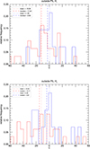 |
Fig. A.1. Histograms of the relative change during the flares (η, in percent of the pre-flare values) of the relative helicity (top) and of the current-carrying helicity (bottom) that are contained in the region outside of the PIL. CME-associated flares are depicted in red, and confined flares are shown in blue. The vertical dotted lines represent the mean values of the respective distributions, and the dashed lines show the median values. |
We immediately notice that the distributions for the CME-associated flares (red curves) are broader compared to the respective ones of Fig. 1. On the contrary, the distributions for the confined flares (blue curves) seem closer to, and more concentrated around 0 compared to the respective distributions of Fig. 1.
More specifically, the mean and median values of the ηHr, out distribution for the CME-associated flares are −13.1% and −11.9%, respectively, not very different from those of ηHr, PIL (−11.8% and −11.4%). The distribution of ηHr, out is quite broader however, as it has an IQR of 28.8%, much larger than the 18.4% of ηHr, PIL. For the confined flares, the mean and median values of ηHr, out are 1.0% and −2.7%, and the IQR is 16.3%, much less than in ηHr, PIL (28.8%).
The ηHj, out distribution for the CME-associated flares is shifted to the right (closer to 0) with respect to Fig. 1, as its mean and median values are −12.2% and −15.2% (−17.5% and −21.6% in Fig. 1). It is also broader, with an IQR of 38.3% (22.4% in Fig. 1). For the confined flares, the ηHj, out distribution is closer to 0 (mean 0.3%, median −3.9%), and more concentrated (IQR of 23.8%), compared to ηHj, PIL (mean −1.4%, median 6.6%, IQR 51.9%). All these values are summarized in Table A.1 along with the values for ηHr, PIL and ηHj, PIL from Table 1 for comparison.
Characteristics (mean, median, and IQR) of the relative flare-related change distributions (ηQ, in units of percents) for the major flares, divided into CME-associated and confined flares.
All Tables
Characteristics (mean, median, and IQR) of the relative flare-related change distributions (ηQ, in units of percents), divided horizontally into CME-associated, confined, and all flares, and divided vertically into major and all flares.
Characteristics (mean, median, and IQR) of the relative flare-related change distributions (ηQ, in units of percents) for the major flares, divided into CME-associated and confined flares.
All Figures
|
Fig. 1. Histograms of the relative change during the flares (η, in percent of the pre-flare values) of the PIL relative helicity (left) and of its current-carrying component (right). CME-associated flares are depicted in red, and confined flares are shown in blue. The vertical dotted lines represent the mean values of the respective distributions, and the dashed lines show the median values. |
| In the text | |
|
Fig. A.1. Histograms of the relative change during the flares (η, in percent of the pre-flare values) of the relative helicity (top) and of the current-carrying helicity (bottom) that are contained in the region outside of the PIL. CME-associated flares are depicted in red, and confined flares are shown in blue. The vertical dotted lines represent the mean values of the respective distributions, and the dashed lines show the median values. |
| In the text | |
Current usage metrics show cumulative count of Article Views (full-text article views including HTML views, PDF and ePub downloads, according to the available data) and Abstracts Views on Vision4Press platform.
Data correspond to usage on the plateform after 2015. The current usage metrics is available 48-96 hours after online publication and is updated daily on week days.
Initial download of the metrics may take a while.