| Issue |
A&A
Volume 704, December 2025
|
|
|---|---|---|
| Article Number | A189 | |
| Number of page(s) | 17 | |
| Section | Interstellar and circumstellar matter | |
| DOI | https://doi.org/10.1051/0004-6361/202449215 | |
| Published online | 16 December 2025 | |
Hydrodynamical models of the β Lyr A circumstellar disc
1
Charles University, Faculty of Mathematics and Physics, Institute of Astronomy,
V Holešovičkách 2,
18000
Prague,
Czech Republic
2
Heidelberger Institut für Theoretische Studien,
Schloss-Wolfsbrunnenweg 35,
69118
Heidelberg,
Germany
★ Corresponding author: This email address is being protected from spambots. You need JavaScript enabled to view it.
Received:
11
January
2024
Accepted:
8
September
2025
Abstract
Aims. We aim to study dynamics of circumstellar discs, with a focus on the β Lyræ A binary system. This system with ongoing mass transfer has been extensively observed using photometry, spectroscopy, and interferometry. All these observations were recently interpreted using a radiation-transfer kinematic model.
Methods. We modified the analytical Shakura-Sunyaev models for a general opacity prescription, and derived radial profiles of various quantities. These profiles were computed for the fixed accretion rate, Ṁ = 2 × 10⁻⁵ M⊙ yr−1, inferred from the observed rate of change of the binary period. More general models were computed numerically, using one-dimensional radiative hydrodynamics, accounting for viscous, radiative, and irradiation terms. The initial conditions were taken from the analytical models.
Results. To achieve the accretion rate, the surface density, Σ, must be much higher (of the order of 104 kg m−2 for the viscosity parameter α = 0.1) than in the kinematic model. Viscous dissipation and radiative cooling in the optically thick regime lead to a high midplane temperature, T (up to 105 K). The accretion disc is still gas-pressure-dominated, with the opacity close to that of Kramers’. To reconcile temperature profiles with observations, we had to distinguish three different temperatures: midplane, atmospheric, and irradiation. The latter two are comparable to observations (30 000-12 000 K). We demonstrate that the aspect ratio, H, of 0.08 can be achieved in a hydrostatic equilibrium, as opposed to previous works considering the disc to be vertically unstable.
Key words: accretion, accretion disks / hydrodynamics / binaries: close / circumstellar matter / stars: individual: beta Lyr A
© The Authors 2025
 Open Access article, published by EDP Sciences, under the terms of the Creative Commons Attribution License (https://creativecommons.org/licenses/by/4.0), which permits unrestricted use, distribution, and reproduction in any medium, provided the original work is properly cited.
This article is published in open access under the Subscribe to Open model. This email address is being protected from spambots. You need JavaScript enabled to view it. to support open access publication.
1 Introduction
The β Lyr A system is an eclipsing binary undergoing rapid mass transfer due to the Roche-lobe overflow; the gainer in the system is an early B star of mass ≈13 M⊙ and the less massive donor is a late B-type star of ≈2.9 M⊙ (Brož et al. 2021). The mass transfer has already switched their primary and secondary roles compared to the initial conditions (Harmanec & Scholz 1993). This likely happened relatively recently; therefore, the mass-transfer rate is still close to its maximum (Deschamps et al. 2013; Lau et al. 2024).
The star was the second eclipsing binary to be discovered and the first ever Be star, with a more than 250 year history of investigations; it is beyond the scope of this introduction to review it in detail (see Harmanec 2002). Due to the ongoing interest in this system, it serves as a prototype for e-Lyræ-type binaries, which are considered natural laboratories of accretion, discs, mass transfer, and mass loss. They are one of the likely progenitors to stellar mergers and supernovæ (Cortés et al. 2024). Even recently this system has often been mentioned as an example or comparison of possible dynamical phenomena in studies of other stars (Rosales et al. 2023; Villaseñor et al. 2023; Nodyarov et al. 2022; Mennickent et al. 2022). There is overwhelming evidence that binary mass transfer also plays a key role in the Be phenomenon for at least some systems (El-Badry et al. 2022), making β Lyr a valuable target for dynamical modelling.
Evidence of a circumstellar material was first presented by Baxandall & Stratton (1930), who noticed additional red-shifted absorption lines just before the middle of the primary eclipse. The first direct interferometric observations were presented by Zhao et al. (2008). Today, there is a broad consensus that the gainer is surrounded by an accretion disc (Mennickent & Djurašević 2013; Mourard et al. 2018; Brož et al. 2021). Observations show the binary’s orbital period P = 12.9440 days (in 2020) (Brož et al. 2021) is increasing at a rate of P = 19 s per year, which corresponds to a mass-transfer rate of M = 2 ∙ 10−5 M⊙ yr−1 (Harmanec & Scholz 1993). The binary also exhibits a second, much longer photometric cycle with a period of 282.4 days (Harmanec et al. 1996), which could be caused by optical-depth changes in the circumstellar disc (a similar variability is seen in AU Mon; Armeni & Shore (2022)). In fact, β Lyr A is atypical among the so-called double-periodic variables (Mennickent 2017) in that it has an evolving period value, while other such systems have a characteristically constant period (Rosales et al. 2023). The preferred distance is 328 pc (Brož et al. 2021), which is slightly different from the associated cluster (294 pc; Bastian 2019).
The optically thick and thin circumstellar material in the system were recently studied by Mourard et al. (2018) and Brož et al. (2021), where a kinematic model was fitted to spectroscopic, light-curve, spectral-energy-distribution (SED), interferometric, and differential-interferometric data. While the accretion disc with a radius of ≈31.5 R⊙ is optically thick, it is surrounded by optically thin material, which results in variable emission-line profiles. Harmanec et al. (1996) proposed that some matter must be propelled in the direction perpendicular to the disc in the form of jets , likely originating where the matter transported from the secondary interacts with the disc. The presence of the jets has been further developed by a number of authors (Ak et al. 2007; Mennickent & Djurašević 2013) and recently considered in the models of Brož et al. (2021).
Hereinafter, we extend their work by taking equilibrium dynamics into consideration. We present an insight into the hydrodynamical state of the disc in the current phase of rapid mass transfer, even though we do not consider a long-term variability of β-Lyræ-type stars (Mennickent & Djurašević 2021; Rojas García et al. 2021).
In Sect. 2, we describe the constraints we place on all our models. In Sect. 3, we give an overview of the derivation of a modification to the well-known analytical models of accretion discs by Shakura & Sunyaev (1973). The classical models generate radial profiles of hydrodynamical quantities of accretion discs around black holes in three different cases. One model assumes a dominance of the radiation pressure over the gas pressure and the Thomson scattering as the opacity source. The other two models assume dominance of the gas pressure; once again assuming an opacity arising from Thomson scattering and the other for Kramers’ opacity. We introduced a general opacity prescription and modified the set of equations so that our model better corresponds to a star as a central object. In Sect. 4, we introduce the numerical, time-dependent, radiation hydrodynamical model based on Chrenko et al. (2017). In Sect. 5, we describe how the models presented in this work are scrutinised. In Sect. 6, we present the specific results obtained for the β Lyr A disc. Finally, in Sect. 7, we discuss these results in the context of other models and compare them to observations presented by Brož et al. (2021).
2 Observational constraints of the β Lyr A disc
To constrain dynamical models of the β Lyr A disc, we used profiles from recent studies of this stellar system, conducted by Mourard et al. (2018) and Brož et al. (2021).
In these studies, authors fitted a series of kinematic models to an extensive set of observations. Hereinafter, we use parameters and profiles from Sect. 3.3 (‘joint compromise model’) of Brož et al. (2021). The profiles may be constructed by inserting parameters from their Table 1 into Equations 11-15. We refer to their results simply as ‘observations’. We now comment on some specific aspects of Brož et al. (2021).
The temperature profile T(r) is best constrained in the outer part of the disc (the system is observed edge-on). The outer boundary temperature reaches just under 12 000 K. The inner boundary temperature is close to the temperature of the star (inferred from spectroscopy to be T* ≈ 30000K), where the slope of the profile is −0.73. The surface-density profile, Σ(r), ranges from approximately 1350 kg m−2 at the inner boundary to approximately 650 kg m−2 at the outer boundary, with a slope of −0.57. However, it should be interpreted as a lower limit, because the total mass of an optically thick medium is not well constrained by observations of a surface (i.e. atmosphere).
During a detailed review of the model used in Brož et al. (2021), we found that they assumed the mean molecular weight μ = 2.36 and the adiabatic index γ = 1.0, which are typical values for cool protoplanetary discs (Kimura et al. 2016). However, the circumstellar environment of the β Lyr A system is much hotter and a composition closer to ionised hydrogen should be assumed.
In fact, one of the converged parameters was the multiplicative factor hcnb, defined as
 (1)
(1)
where H denotes the actual pressure scale height of the disc and Heq the pressure scale height in a vertical hydrostatic equilibrium. The best-fit value was hcnb = 3.8, and they interpreted this as a disc being vertically unstable. We suspect that at least a part of the increase is due to the choice of μ and γ. Hence, we adjusted the values in the Brož et al. (2021) model as follows: hcnb = 1.0, μ = 0.5, and γ = 1.4, as corresponds to ionised hydrogen and vertical hydrostatic equilibrium. We also recomputed the radial profiles of pressure scale height, density, and pressure (from the converged temperature profile); note that we did not run the convergence again.
The profiles are somewhat shifted, therefore we suspect the original high hcnb has probably also other causes than the choice of μ and γ. We refer to these shifted profiles throughout the text as ‘adjusted observations’. We emphasise that we do not claim that the Brož et al. (2021) disc must be in vertical equilibrium, we used this modified model as a hydrostatic limit to the Brož et al. (2021) disc and we plot it for reference next to our results.
In our work, we adopted several values from Brož et al. (2021) as fixed parameters (see Table 1). In addition, we take dynamics into consideration, the main dynamical constraint is the mass transfer rate between the two stars. We assumed that the total mass is conserved during the transfer.
Fixed parameters adopted from Brož et al. (2021).
3 Analytical models
In this section, we derive a modification to the analytical models of Shakura & Sunyaev (1973) to make them better applicable to a case where the central object is a star (not a black hole)1.
3.1 Derivation of the analytical models
We now discuss the derivation in detail by listing all the equations. We followed the main steps of the derivation from Shakura & Sunyaev (1973), but for a more general case, adopting adjustments to the set of equations. For a comprehensive description of assumptions behind the models see the original paper (Shakura & Sunyaev 1973). The surface density, Σ, is obtained by integrating the volume density over the vertical extent of the disc, which is equal to multiplying by a factor of two times the disc’s pressure scale height, H:
 (2)
(2)
The pressure scale height, H, assuming hydrostatic equilibrium is given by the ratio of the sound speed, cs, and the Keplerian angular velocity, ΩK (Pringle 1981):
 (3)
(3)
For the sound speed, a general formula in an isothermal approximation is (Shakura & Sunyaev 1973)
 (4)
(4)
We assumed Keplerian rotation in the disc. Assuming that the central star will rotate with a sub-Keplerian velocity (otherwise it would be at its stability limit, but Be stars are shown to rotate at sub-critical velocities (Rivinius et al. 2013) implies that the angular velocity curve, Ω(r), must have a maximum located at or beyond the inner edge of the disc; that is,  . This boundary condition then introduces a ‘bending’ term into the equation for the surface density, Σ (Pringle 1981):
 (5)
(5)
where ν is the kinematic viscosity.
Plugging into a more general equation for viscous energy dissipation, Qvisc, Pringle (1981) derived
 (6)
(6)
The models assume radiative energy losses only from the two faces of the disc. This is given by the Stefan-Boltzmann law,
 (7)
(7)
where the vertical temperature profile is approximated by a model atmosphere according to Hubeny (1990) in an optically thick limit. The ‘effective’ optical depth is then given by
 (8)
(8)
The optical depth, τopt, of the vertical layer is approximated as in Chrenko et al. (2017):
 (9)
(9)
where κ is opacity and the Ck factor accounts for the opacity change above the midplane as suggested by comparisons of 3D and 2D models (Müller & Kley 2012). In the case of our results, generated by these analytical models, we always set the factor to Ck = 0.6, as suggested for hydrodynamic simulations by Chrenko et al. (2017).
The models arise from an assumed fundamental energy balance; that is, all the energy generated by viscous friction is radiated away. This is given by
 (10)
(10)
The kinematic viscosity, ν, is parameterised with α, which can be introduced by assuming that angular momentum is exchanged between rings of the disc via eddies with a limit to the size given by the vertical extent of the disc and velocity given by the local sound speed, cs, in the disc (Pringle 1981):
 (11)
(11)
where H is the disc pressure scale height.
As a generalisation to the models by Shakura & Sunyaev (1973), we used a more general form of an opacity prescription parameterised by three constants, κ0, A, and B,
 (12)
(12)
a choice of the constants then defines a specific model with a specific dominant opacity source.
The equation of state is the same as the one for stellar matter since the source of the matter is a binary mass transfer. It combines ideal gas and radiation pressure P = Pg + Pr and is in its full form given by
 (13)
(13)
where σB is the Stefan-Boltzmann constant, c the speed of light, kB the Boltzmann constant, μ the mean molecular weight, mp the mass of the proton, T the midplane temperature, and ρ the midplane density. For simplicity, we assumed the disc is made of pure ionised hydrogen and chose μ = 0.5.
In order to obtain prescriptions for the radial profiles, we can apply different assumptions to the equation of state about the relative importance of gas pressure and radiation pressure. That is, we actually derive three different classes of models, each based on a single assumption, specifically Pg ≈ Pr, Pg ≫ Pr, and Pg ≪ Pr.
A careful inspection of the results of Brož et al. (2021) led us to consider all three assumptions as possibly applicable to the system. The Brož et al. (2021) profiles were given for ρ and T (as referenced in Sect. 2). Applying the equation of state (Eq. (13)) gives contributions from gas and radiation pressure. The resulting pressure contributions are of approximately equal magnitudes. However, we must further take into account the observed ρ profile, which is a lower limit; hence, the possibility of a gas-pressure-dominated disc cannot be excluded. Moreover, there are still uncertainties in the T profile. Especially in the inner part of the disc (Mourard et al. 2018), the profile is weakly constrained, due to the ∝ T4 proportionality, we should not a priori rule out radiation-pressure-dominated discs.
3.2 Gas-pressure-dominated discs (Pg ≫ Pr)
The first class is based on the assumption that the gas pressure dominates over the radiation pressure, Pg ≫ Pr. Neglecting radiation pressure in Eq. (13), we effectively recover the ideal gas equation of state.
To simplify notation, we denote the often-appearing sum of exponents as
 (14)
(14)
Then,
 (15)
(15)
 (16)
(16)
 (17)
(17)
 (18)
(18)
 (19)
(19)
 (20)
(20)
 (21)
(21)
 (22)
(22)
where opacity-independent constants (subscript 0) are defined as
 (23)
(23)
 (24)
(24)
 (25)
(25)
 (26)
(26)
We obtained prescriptions for the profiles of hydrodynamical quantities dependent on six input parameters. The form of the prescriptions is similar to the classical models. Each has four main parts; a scaling constant (with the index*), scaling by some powers of the input parameters (α, M*, Ṁ), a power law of the radial coordinate, and the bending term introduced Eq. (5). For the sake of intuition, note that the bending factor always has the same exponent as the mass-transfer rate Ṁ. The exponents in each term are dependent on the parameters defining the specific opacity prescription. The scaling constants do not have a specific meaning; however, individually, we may notice that far away from the star, all prescriptions reduce to simple power laws of the radial coordinate.
3.3 Gas and radiation pressures of equal magnitudes (Pg ≈ Pr)
The second class considers both sources of pressure of approximately equal importance, Pg ≈ Pr. In practice, we used
 (27)
(27)
Again, we denote the often-appearing sum of exponents, D, in this section. It corresponds to
 (28)
(28)
Then,
 (29)
(29)
 (30)
(30)
 (31)
(31)
 (32)
(32)
 (33)
(33)
 (34)
(34)
 (35)
(35)
 (36)
(36)
where opacity-independent constants are defined as
 (37)
(37)
 (38)
(38)
 (39)
(39)
 (40)
(40)
The obtained prescriptions are composed of the same terms as those described in Sect. 3.2, yet the power-law exponents contain other combinations of the opacity-specific constants (A,B). The definitions of the scaling constants are also different.
3.4 Radiation-pressure-dominated discs (Pg ≪ Pr)
The third class includes models of radiation-pressure-dominated discs (Pg ≪ Pr). As before, we neglected the other part of the equation of state (Eq. (13)), reducing it to the radiationpressure equation of state. Following Shakura & Sunyaev (1973), to obtain a temperature profile we calculate the energy density, e, of radiation inside a layer,
 (41)
(41)
and a plug in the Stefan-Boltzmann law,
 (42)
(42)
Again, we denote the often-appearing sum of exponents, D. In this section, it corresponds to
 (43)
(43)
Then,
 (44)
(44)
 (45)
(45)
 (46)
(46)
 (47)
(47)
 (48)
(48)
 (49)
(49)
 (50)
(50)
 (51)
(51)
where opacity-independent constants for this class are defined as
 (52)
(52)
 (53)
(53)
 (54)
(54)
 (55)
(55)
Again, we obtained the same terms as in Sect. 3.2, yet with different power-law exponents and different scaling constants.
4 Numerical model
In order to constrain the timescales of evolution, we also computed 1D hydrodynamical simulations of the β Lyr A disc with an Eulerian solver on a polar staggered mesh (Van Leer 1977; Stone & Norman 1992; Masset 2000; Chrenko et al. 2017). Since our analytical models are based on a few strict assumptions, we used the numerical model to verify their validity in this specific case, as described in Sect. 5. We omit a comprehensive description of the code (FARGO or FARGO_THORIN), but we introduce the respective set of fluid equations in Appendix A. We now note some of the specifics of the model that are relevant for interpreting our results.
Energy equation. The calculation of energy balance is more detailed in the numerical model (cf. Eq. (10)). Energy dissipation by viscous forces is determined by
 (56)
(56)
where the viscous stress tensor, π, is calculated according to Masset (2002). Radiative losses Qrad from the faces of the disc are also described for optically thin matter, using the effective opacity (Hubeny 1990; Chrenko et al. 2017):
 (57)
(57)
This was then used in the same Stefan-Boltzmann model as in the analytical models (Eq. (7)). Additionally, irradiation from the central star is included and assumed to occur through the disc’s faces (Chrenko et al. 2017):
 (58)
(58)
where Tirr denotes the effective temperature of the radiation falling onto the disc’s surface. It is calculated by the projection of the radiative flux on the surface:
 (59)
(59)
where A denotes the disc’s albedo and δ is an estimate of the incident angle (Chrenko et al. 2017).
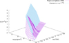 |
Fig. 1 Rogers & Iglesias (1992) 2D opacity function (magenta) approximated by a plane (in a logarithmic plot) in the interval corresponding to Kramers’ opacity (cyan). |
5 Methodology
We explored the parameter space of the modified Shakura-Sunyaev models (derived in Sect. 3), in particular the part that could be relevant to the studied β Lyr A disc. The results from the application of these analytical models were then used as initial conditions for simulations with the numerical model, which is introduced in Sect. 4. The resulting radial profiles were then compared to Brož et al. (2021), both qualitatively and quantitatively. In this section, we define the specifics of our approach.
5.1 The choice of opacity
When applying the analytical models to a system, after choosing an assumption about pressure, the values of six input parameters (α, Ṁ, M*, κ0, A, B) are needed to generate radial profiles. The three constants defining an opacity approximation are a generalisation of the classical Shakura-Sunyaev models.
We adopted the 2D opacity function κ = κ(ρ, T) from Rogers & Iglesias (1992). For defined regions, we found approximations in the form of Eq. (12). Initially, we focused on regions that were indicated as possibly corresponding to the disc discussed by Brož et al. (2021), but as our investigation progressed we iterated our choices according to our intermediate results. The approximations were optimised by converging parameters κ0, A, and B from Eq. (12) using the least-squares method (as in Fig. 1).
Overview of modified Shakura-Sunyaev models for β Lyr A disc.
5.2 Scrutiny of the analytical models
We observe the criteria listed below when judging the usefulness of the individual analytical models.
We checked the consistency of the calculated profiles with assumptions under which they were derived. Two types of possible inconsistencies are observed. First, each class of models is dependent on one of three assumptions about gas and radiation pressure. Second, the individual models are generated by a specific opacity approximation (through κ0, A and B), which are only valid in the specific part of the T - ρ space.
In our models, we treated α as a free parameter. As we are aware of the uncertainty that goes along with our assumptions, we prefer models that fulfil the consistency discussed above for a wide range of α values. We refer to the ‘stability’ of the consistency.
We compared the values in the computed profiles with the observations and adjusted observations. This is again α-dependent.
The Brož et al. (2021) profiles are essentially power laws. As noted in Sect. 3, the modified Shakura-Sunyaev profiles are also approximated by power laws for r ≫ 1. We thus compare the exponents of the temperature profiles; the observed temperature profile is proportional to T ∝ r−0.73 (Brož et al. 2021).
5.3 Time-dependent numerical simulations with general opacity tables
A final model of the β Lyr A system is obtained by more self-consistent numerical simulations, where the results from the analytical models are used as initial conditions. This choice improves the chances of doing away with initial transients in the simulation as efficiently as possible. When we demonstrate the internal consistency of the analytical models for specific parameters, it also serves as justification for the choice of included physics in the numerical model (e.g. the equation of state).
In these simulations, we did not assume a single power-law opacity prescription in advance, as in the analytical models; instead, we used more general opacity tables (e.g. Zhu et al. 2012; Bell & Lin 1994). The opacity table is made up of several power-law approximations, with the advantage that an opacity prescription is chosen at each time step, based on the local conditions that arise during the simulation (corresponding ρ and T).
This step to numerical simulations is necessary for a number of reasons; namely, (i) the analytical models were derived assuming a steady-state Keplerian disc, and time-dependent simulations without an enforced velocity profile can test the validity of this assumption in the case of the studied system; (ii) general opacity tables allow for the opacity regime to be coupled to the physical state of the system; and (iii) the influence of phenomena such as stellar irradiation that are not included in the analytical model should be also assessed. The profiles from this model were then used to interpret the observationally constrained profiles of Brož et al. (2021).
6 Results
Hereinafter, we present our main results from both the analytical and numerical models; alternative models that we eventually rejected are presented in Appendices B and C. All presented analytical models are summarised in Table 2, but in the following we consider the models belonging to the class, which led to the best, self-consistent results (i.e. gas-pressure-dominated, with Kramers’ opacity).
6.1 Gas-pressure-dominated analytical models of the β Lyr A disc
Here, we explain how we applied gas-pressure-dominated profiles from Eqs. (15)-(22) for a specific choice of the opacity prescription.
6.1.1 Kramers’ opacity
In Fig. 1, for illustration purposes, we plot the 2D opacity function (Rogers & Iglesias 1992) and the approximation of the region approximately corresponding to Kramers’ opacity (Eq. (60)), which is valid for a wide range of temperatures:
 (60)
(60)
The resulting hydrodynamical profiles are plotted in Fig. 2.
The profiles generated by the gas-pressure-dominated model with Kramers’ opacity are consistent with the assumptions under which the model was derived for all tested values of the α parameter.
The temperature profiles generated by the Kramers’ model (for all α parameters) are significantly higher than in the observed profiles. The analytic model generates a hotter disc with only viscous dissipation, while in reality stellar irradiation serves as an additional energy source. The case of the theoretical limit, α = 1.0 (Shakura & Sunyaev 1973), approaches the observed profile, but the agreement is still not satisfactory.
An inspection of Table 2 shows that this model produces the qualitatively most compatible temperature profile, T ∝ r−0.75. This similarity was also hinted at by Brož et al. (2021).
The model shows significantly higher surface-density profiles, Σ, for α = 0.1 and α = 0.01. The values of the Σ profiles are over ten and 100 times larger than the observations. For reference, in Fig. 2a we plot Σ profiles for the observations and adjusted observations, multiplied by a factor of 100. Even for the theoretical limit of α = 1.0, it is still about four times larger.
We show the pressure profiles in Fig. 2c. Due to the high temperatures and densities in the disc, both gas-pressure and radiation-pressure values are significantly higher than can be calculated from the observed profiles. For reference, in Fig. 2c we plot gas pressure profiles calculated from the observations and adjusted observations assuming a 100 times larger density.
Kramers’ model generates aspect ratios (for α = 1.0,0.1,0.01) between the observations and adjusted observations, as demonstrated in Fig. 2d. This is due to the high midplane temperatures, allowing the H profile given in Brož et al. (2021) to be reached in a hydrostatic equilibrium.
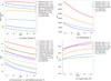 |
Fig. 2 Radial profiles of surface density (a), temperature (b), gas and radiation pressures (c), and aspect ratio of the β LyræA disc for a modified Shakura-Sunyaev model, which is gas-pressure-dominated and has Kramers’ opacity. The midplane temperatures and surface densities are significantly higher than the observed values. This also generates significantly higher pressure profiles. The observed aspect ratio is reached in hydrostatic equilibrium. |
6.1.2 Implications from all analytical models
From the application of the modified Shakura-Sunyaev models (Table 2), we can already draw several conclusions. The models based on assuming gas-pressure dominance are robustly consistent, whilst other classes of models are either contradictory to their own assumptions or their consistency is unstable. We take this to be an argument that gas pressure plays a dominant role in the disc.
None of the models match the densities or temperatures of the observationally constrained profiles well, without choosing the extreme case of α = 1.0. The generated densities and temperatures tend to be significantly higher. Considering the criteria from Sect. 5.2, we can see the gas-pressure-dominated disc with α = 0.1 and Kramers’ opacity as the preferred model.
Time-dependent numerical-model input parameters.
6.2 Time-dependent model with the Zhu et al. (2012) opacity table
For the preferred analytical model (gas-pressure-dominated Kramers’ opacity, α = 0.1), we constructed a corresponding numerical model. However, we used the general opacity table by Zhu et al. (2012) and input parameters given in Table 3. Our results are presented in Fig. 4.
The disc reached a steady state within one year of simulation time and remained without temporal evolution for the rest of the simulation time (the run was terminated after 2 · 103 days). We calculated the viscous timescale profile and found a range from about tνin = 0.5 years in the inner part of the disc to about tνout = 3 years in the outer part.
According to the opacity table, the values of κin ≈ 100 cm−2 g−1 in the inner part of the disc and κout ≈ 101 cm−2g−1 in the outer part were reached, without any opacity transitions in the radial profile. This closely resembles a profile generated by a simulation with the prescription  , which was previously used for one of the gas-pressure-dominated analytical models (‘high-temperature’ model); we note that it should be considered a slight variation of Kramers’ opacity regime.
The disc rotates with a slightly sub-Keplerian velocity due to a radial pressure gradient in the disc; however, the deviations are minor. The radial velocities are dependent on the efficiency of the angular momentum redistribution and are coupled to the Σ radial profile via the fixed mass transfer. Radial velocities in the disc range from about 600 m s−1 on the inner boundary to 400 m.s−1 on the outer boundary. Due to the high temperatures and densities, the model can reach a good agreement with the observed aspect ratio, even under the assumption of a vertical hydrostatic equilibrium.
The Σ problem. Comparing the surface-density profile and the Brož et al. (2021) observationally constrained profile, the densities from our numerical simulation reach values almost 100 times larger. This discrepancy in the profiles of surface density is still acceptable. As discussed in Sect. 2, the observed Σ profile is a lower limit to densities that could explain the observations. Taking dynamics into consideration, we require a fixed amount of matter that must be transferred through the disc (determined by Ṁ, vr, and α).
The temperature problem. The midplane temperature of the disc from our numerical simulation is around three times higher than the observed profile of Brož et al. (2021), which is the most dramatic discrepancy. An important aspect to consider is that each approach has completely different assumptions about the vertical temperature profile of the disc. These are as follows:
rož et al. (2021) assumed a vertically isothermal atmosphere. The disc is optically thick; hence, the observations by which they constrain their model are observations of the atmosphere. Inevitably, they infer the midplane temperature as being equal to the atmospheric temperature. They also allow for a temperature inversion in their model, so the outer atmosphere can even be hotter than the midplane temperature.
Chrenko et al. (2017) assumed the atmosphere model derived by Hubeny (1990). The atmosphere dims the midplane, and the face of the disc radiates with an atmospheric temperature (Eq. (7)), which is lower.
If we reject the assumption of an isothermal atmosphere and re-interpret the temperature profile of Brož et al. (2021) as the measured temperature of the atmosphere, then it should be compared to the atmospheric temperature Teff inferred from the midplane temperature according to Hubeny (1990):
 (61)
(61)
Further, a theoretical upper thermodynamic limit of Teff could be the irradiation temperature, Tirr. Even though Teff and Tirr are of comparable magnitudes, the agreement is still poor. The atmospheric temperature profile, Teff, is now lower than the observed profile and surpasses the limiting Tirr profile in the inner part of the disc.
Solution 1: temperature inversion in the vertical stratification These further discrepancies point to a more complex vertical temperature profile. In Brož et al. (2021), an inversion in the vertical temperature profile was considered. In Fig. 3, we demonstrate how an inversion, for example due to non-thermal irradiation, could explain the discrepancies between temperature profiles from the observations and from our numerical models. With increasing distance from the midplane, the temperature decreases approximately according to the Hubeny (1990) model. At the level of the inversion, the temperature starts growing again, up to where the matter becomes optically thin, where it reaches the observed value. Similar temperature inversions can be seen in models of other Be stars (e.g. in decretion discs; Granada et al. 2021). Alternative solutions are discussed in Appendix C.
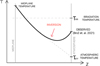 |
Fig. 3 Sketch of how presence of temperature inversion in vertical profile of disc could reconcile computed midplane temperature (Tmid) profile, the observed temperature profile and the calculated atmospheric Teff and irradiation Tirr profiles. |
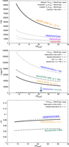 |
Fig. 4 Temperature, T(r) (top), surface density, Σ(r) (middle), and aspect ratio, H(r) (bottom), profiles of the time-dependent numerical model (from Table 3 with the Zhu et al. (2012) general opacity table). The midplane temperatures are significantly higher than the observations. The calculated atmospheric temperatures, Teff, and irradiation temperatures, Tirr, are of comparable magnitudes to the observations, but the correspondence between the temperature profiles is not satisfactory. Surface densities from the model are almost 100 times the observed value. The observed aspect ratio is reached in hydrostatic equilibrium. |
7 Discussion
Finally, we discuss more general implications of our modelling of the β Lyr A disc. These are listed below.
Viscosity: Overall, our preferred (time-dependent) model was obtained for α ≈ 0.1; there, we tested different orders of magnitude of α and did not perform any ‘fine-tuning’. This value is consistent with evidence for fully ionised thin accretion discs (values in literature given at 0.1-0.3; King et al. (2007); Ghoreyshi et al. (2018); Granada et al. (2021). The model of the limit case of α = 1.0 was also considered as a possible way to reconcile models and observations (Appendix C.4), but it is not preferred because without a clear idea of how this value could be obtained from the microphysics of viscosity or higher dimensional macroscopic phenomena in the disc (Boffin 2008), it is something of an arbitrary choice without objective justification. Possible dynamical phenomena contributing negative angular momenta such as spiral waves must be explored with 2D and 3D simulations. In all our simulations, we used α, which is constant with the radial distance. In principle, α may vary across the disc; for example, Flock et al. (2016) proposed a formula that increases α in zones where the gas is hot enough to be sufficiently ionised for the magneto-rotational instability to occur. However, β Lyr A is hot enough to be ionised everywhere (we obtain a constant α again). No quantities show any ‘jumps’ or regime transitions; hence, only some weak power laws may be considered. The effect on the result is not likely to be dramatic. The influence of α on the equilibrium state can be estimated from our modified Shakura-Sunyaev models, for example for the temperature profile in the case of a gas pressure dominated disc with Kramers’ opacity,  .
.
Conservation of mass: One of the key parameters of our model is the fixed mass-transfer rate, Ṁ, the value of which was inferred from the period change of the binary, assuming mass conservation. It is to be noted that in reality, the conservation of mass is imperfect. Accretion of angular momentum from the disc may be the origin of the rotational velocities of Be stars. The spin-up of the gainer can lead to super-synchronous rotation, which modifies the Roche equipotentials, where the lobe moves closer to the star (Plavec 1958). This implies that overflows and, hence, nonconservative mass transfer on the gainer’s side are more likely (Lau et al. 2024). Documented jets and the optically thin material surrounding the system are further indications of some mass loss (Harmanec et al. 1996; Brož et al. 2021; Villaseñor et al. 2023). The value of Ṁ has a significant influence on the models (e.g. for the gas-pressure-dominated analytical model assuming Kramers opacity,  ); hence, the amount of optically thin matter around the system needs to be constrained.
Timescales. In our time-dependent models, the disc relaxed quite quickly and remained as such for the rest of the simulation time (a multiple of viscous timescales (Pringle 1981); tν ≈ 0.5 yr at the inner boundary to tν ≈ 3 yr at the outer boundary). A steady-state configuration therefore seems a probable configuration for the disc. We highlight the fact that in the presented alternative models a steady state was also reached.
Orbital velocities. The radial pressure gradient in our numerical simulations resulted in only a slightly sub-Keplerian rotation. For many practical purposes, it is still valid to approximate the disc as Keplerian. When also considering the steady state reached, the results of the time-dependent simulations fulfil the assumptions of the applied analytical models (Shakura & Sunyaev 1973). This is in agreement with the broad consensus that Be stars are surrounded Keplerian discs (see the review by Rivinius et al. (2013). Furthermore, there is a general agreement between our preferred analytical and numerical models, which is encouraging for the application of equilibrium models.
Opacity: The preferred analytical models were obtained for Kramers’ opacity; a more general opacity table by Zhu et al. (2012) also produced an opacity profile with values close to the Kramers’ opacity. The disc exhibits no opacity transitions. The viscosity parameter α ≈ 0.1 preferred in this study is common in ionised accretion discs; hence, a combination of free-free (bremsstrahlung) and bound-free (photoionisation) absorption -both approximated by Kramers’ opacity law- is a corresponding candidate for the main opacity source (Zel’dovich & Raizer 2012). This is consistent with the density (ρ ≈ 10−5 kg.m−3) and temperature T ≈ 104−105 K) profiles in our model of the disc interior (Fig. 4), for which the Saha equation predicts the ionisation fraction safely above 0.5.
Moreover, the vertical opacity profile has a substantial impact on the disc (Appendix C.3) and should be considered with care. Here, we assumed the same opacity regime within the whole vertical extent, but we introduced the integrated effect of the κ(z) dependency through the Ck factor in calculating optical depth (Eq. (9)). Yet, for a more precise result, the vertical opacity profile needs to be modelled self-consistently, hand in hand with the vertical temperature profile.
Pressure. The analytical models are consistent for a wide range of opacities and values of α with their own assumptions only when Pg ≫ Pr is assumed. The (unmodified) numerical model (Chrenko et al. 2017) contains an ideal-gas equation of state (Eq. (A.4)), so it is based on the same assumption. We also considered an additional increase due to radiation pressure, but its influence is indeed minor.
Surface densities and radial velocities: Due to the fixed masstransfer rate, the surface-density profile and radial-velocity profile are strongly coupled in our models. Radial velocities in the disc are of the order of 102ms−1. In both the analytical and numerical models (computed for α = 0.1), we obtain surface densities of the order of 104 kg m−2 throughout the disc. This is close to 100 times the observed value (which is only a lower limit to the real densities of the optically thick matter; Brož et al. 2021). An improved model that would consider nonconservative mass transfer (hence lower Ṁ, while keeping Ṗ) would allow for both lower surface densities and lower radial velocities without a significant influence on the observables of the disc.
Temperature profile. Both our preferred models (for α = 0.1) indicate high midplane temperatures, close to T ≈ 105 K at the inner boundary to T ≈ 3 · 104 K at the outer boundary. This is significantly higher than the observed temperatures of Brož et al. (2021). In fact, the latter values were derived from fitting observations of the radiative atmosphere of the disc (at the boundary of the optically thick matter). When we computed the atmospheric temperatures from our numerical model (under the assumption of the atmosphere by Hubeny (1990)) and considered the possibility of temperature inversion in the upper atmosphere, we obtained the magnitudes comparable to the observations (i.e. 3 . 104 to 1·104 K). The inversion is consistent with the strong Hα emission. Temperature inversions are features seen in other Be star models (e.g. in Granada et al. (2021). We thus emphasise the need for higher dimensional models also in the case of β Lyr A.
Studies of similar systems report lower temperatures; Mennickent & Djurašević (2021) observations of a e-Lyræ-type binary show disc temperatures of the order of 103 K. However, they also demonstrate that the temperature has a positive correlation with the mass-transfer rate, in agreement with our analytical model. The lower temperatures are thus arising due to the lower mass of the binary (4.83 + 1.06 M⊙). Similarly, the Granada et al. (2021) model of the decretion disc of the Be shell star 1 Del shows temperatures of the order of 103 K, even in the hottest parts of the interior. This is because the disc has densities 1000 times lower and radial outflow velocities 10-100 slower than in our model of β Lyr A.
As an alternative to the presence of an inversion, the possibility of vertical convective energy transport should be explored. This has been shown as a possibility in circumstellar discs (Müller & Kley 2012). If present in the β Lyr A disc, it would constitute a more effective cooling mechanism. The more gradual temperature gradient could allow for lower midplane temperatures while keeping similar atmospheric temperatures.
Aspect ratio. Due to the high midplane temperatures and densities, the observed aspect ratio of H/r ≈ 0.08 can now be reached in a hydrostatic equilibrium. The sensitivity of H/r on the individual input parameters can be also inferred from our analytical models. Moreover, if the contribution of radiation pressure is considered, the vertical extent of the disc increases further (Montesinos et al. 2021).
8 Conclusions
We present analytical and numerical hydrodynamical models of the circumstellar disc around the gainer of the β Lyr A system at the phase of rapid mass transfer. The consistency check of the analytical models points to gas pressure being dominant in the disc; the contribution of the radiation pressure could be at most 10%. We estimated the viscosity parameter governing the angular-momentum redistribution to be close to α ≈ 0.1. This is within the range of typical values of highly ionised accretion discs. Both the analytical models and the general opacity tables indicate that the dominant source of opacity in the optically thick disc is free-free and bound-free absorption, as modelled by Kramers’ opacity (see Sect. 6.1.1 for details).
All our time-dependent models show the disc is in a steady state with only slightly sub-Keplerian rotational velocities. In our model, the mass transfer rate of Ṁ = 2 × 10⁻⁵ Ṁ⊙ yr−1 is achieved with the surface densities ranging from 20 000 to 60 000 kg m−2 and the radial velocities of the order of 100 m s−1. Temperatures in the midplane reach 30 000 to over 90 000 K; the respective Shakura-Sunyaev models predict a power-law exponent of −0.75. Given the remaining ‘tension’ between the density and temperature profiles (discussed in Sect. 6.2), we predict that the vertical temperature profile is likely complex, with a temperature inversion in the top layers. A comparison to fitted observations shows that vertical hydrostatic equilibrium can be preserved with an aspect ratio H/r of 0.08. On top of the steady state, a timescale comparison shows there is a possibility of spiral waves, which would transport a negative angular momentum to the inner parts of the disc.
As a continuation of this work, we propose studying the β Lyræ A system assuming a non-conservative mass transfer and to discuss a possibility of temporal evolution of the system’s intrinsic parameters (similarly to in Mennickent & Djurašević (2021)). Several variations of the numerical model were suggested to address the discrepancy in the temperature profile: a convective instability, a temperature inversion in the vertical direction, and edge-on irradiation from the central star. Other phenomena such as spiral waves should be studied with 2D and 3D simulations.
Acknowledgements
M.B. was supported by the Czech Science Foundation grant GA21-11058S. K.V. is a fellow of the International Max Planck Research School for Astronomy and Cosmic Physics at the University of Heidelberg (IMPRS-HD) and acknowledges financial support from IMPRS-HD. During revisions K.V. was supported by the Klaus Tschira Foundation.
References
- Ak, H., Chadima, P., Harmanec, P., et al. 2007, A&A, 463, 233 [CrossRef] [EDP Sciences] [Google Scholar]
- Armeni, A., & Shore, S. N. 2022, A&A, 664, A103 [NASA ADS] [CrossRef] [EDP Sciences] [Google Scholar]
- Bastian, U. 2019, A&A, 630, L8 [NASA ADS] [CrossRef] [EDP Sciences] [Google Scholar]
- Baxandall, F., & Stratton, F. 1930, The Spectrum of B. Lyrae, Annals of the Solar Physics Observatory, Cambridge [Google Scholar]
- Bell, K. R., & Lin, D. N. C. 1994, ApJ, 427, 987 [NASA ADS] [CrossRef] [Google Scholar]
- Boffin, H. 2008, Spiral Waves in Accretion Discs - Theory, 69 [Google Scholar]
- Brož, M., Mourard, D., Budaj, J., et al. 2021, A&A, 645, A51 [EDP Sciences] [Google Scholar]
- Chrenko, O., Brož, M., & Lambrechts, M. 2017, A&A, 606, A114 [Google Scholar]
- Cortés, C. C., Garcés, J., Mennickent, R. E., & Djurašević, G. 2024, AJ, 167, 17 [Google Scholar]
- Deschamps, R., Siess, L., Davis, P. J., & Jorissen, A. 2013, A&A, 557, A40 [NASA ADS] [CrossRef] [EDP Sciences] [Google Scholar]
- ERl-Badry, K., Conroy, C., Quataert, E., et al. 2022, MNRAS, 516, 3602 [NASA ADS] [CrossRef] [Google Scholar]
- Flock, M., Fromang, S., Turner, N. J., & Benisty, M. 2016, ApJ, 827, 144 [CrossRef] [Google Scholar]
- Ghoreyshi, M. R., Carciofi, A. C., Rímulo, L. R., et al. 2018, MNRAS, 479, 2214 [Google Scholar]
- Granada, A., Jones, C. E., & Sigut, T. A. A. 2021, ApJ, 922, 148 [Google Scholar]
- Harmanec, P. 2002, Astron. Nachr., 323, 87 [NASA ADS] [CrossRef] [Google Scholar]
- Harmanec, P., & Scholz, G. 1993, A&A, 279, 131 [NASA ADS] [Google Scholar]
- Harmanec, P., Morand, F., Bonneau, D., et al. 1996, A&A, 312, 879 [Google Scholar]
- Hubenÿ, I. 1990, ApJ, 351, 632 [NASA ADS] [CrossRef] [Google Scholar]
- Kimura, S. S., Kunitomo, M., & Takahashi, S. Z. 2016, MNRAS, 461, 2257 [NASA ADS] [CrossRef] [Google Scholar]
- King, A. R., Pringle, J. E., & Livio, M. 2007, MNRAS, 376, 1740 [NASA ADS] [CrossRef] [Google Scholar]
- Lau, M. Y. M., Hirai, R., Mandel, I., & Tout, C. A. 2024, ApJ, 966, L7 [NASA ADS] [CrossRef] [Google Scholar]
- Masset, F. S. 2000, A&AS, 141, 165 [NASA ADS] [CrossRef] [EDP Sciences] [Google Scholar]
- Masset, F. S. 2002, A&A, 387, 605 [NASA ADS] [CrossRef] [EDP Sciences] [Google Scholar]
- Mennickent, R. E. 2017, Serb. Astron. J., 194, 1 [NASA ADS] [CrossRef] [Google Scholar]
- Mennickent, R. E., & Djurašević, G. 2013, MNRAS, 432, 799 [NASA ADS] [CrossRef] [Google Scholar]
- Mennickent, R. E., & Djurašević, G. 2021, A&A, 653, A89 [NASA ADS] [CrossRef] [EDP Sciences] [Google Scholar]
- Mennickent, R. E., Djurašević, G., Petrovic, J., et al. 2022, A&A, 666, A51 [NASA ADS] [CrossRef] [EDP Sciences] [Google Scholar]
- Montesinos, M., Cuello, N., Olofsson, J., et al. 2021, ApJ, 910, 31 [CrossRef] [Google Scholar]
- Mourard, D., Brož, M., Nemravová, J. A., et al. 2018, A&A, 618, A112 [NASA ADS] [CrossRef] [EDP Sciences] [Google Scholar]
- Müller, T. W. A., & Kley, W. 2012, A&A, 539, A18 [Google Scholar]
- Nodyarov, A. S., Miroshnichenko, A. S., Khokhlov, S. A., et al. 2022, ApJ, 936, 129 [Google Scholar]
- Plavec, M. 1958, in Liege International Astrophysical Colloquia, 8, Liege International Astrophysical Colloquia, 411 [Google Scholar]
- Pringle, J. E. 1981, 19, 137 [Google Scholar]
- Rivinius, T., Carciofi, A. C., & Martayan, C. 2013, A&A Rev., 21, 69 [NASA ADS] [CrossRef] [Google Scholar]
- Rogers, F. J., & Iglesias, C. A. 1992, ApJ, 401, 361 [NASA ADS] [CrossRef] [Google Scholar]
- Rojas García, G., Mennickent, R., Iwanek, P., et al. 2021, ApJ, 922, 30 [Google Scholar]
- Rosales, J. A., Mennickent, R. E., Djurašević, G., et al. 2023, A&A, 670, A94 [NASA ADS] [CrossRef] [EDP Sciences] [Google Scholar]
- Shakura, N. I., & Sunyaev, R. A. 1973, A&A, 24, 337 [NASA ADS] [Google Scholar]
- Stone, J. M., & Norman, M. L. 1992, ApJS, 80, 753 [Google Scholar]
- Van Leer, B. 1977, J. Computat. Phys., 23, 276 [NASA ADS] [CrossRef] [Google Scholar]
- Villaseñor, J. I., Lennon, D. J., Picco, A., et al. 2023, MNRAS, 525, 5121 [CrossRef] [Google Scholar]
- Zel’dovich, Y., & Raizer, Y. 2012, Physics of Shock Waves and High-Temperature Hydrodynamic Phenomena, Dover Books on Physics (Dover Publications) [Google Scholar]
- Zhao, M., Gies, D., Monnier, J. D., et al. 2008, ApJ, 684, L95 [CrossRef] [Google Scholar]
- Zhu, Z., Hartmann, L., Nelson, R. P., & Gammie, C. F. 2012, ApJ, 746, 110 [Google Scholar]
The Python scripts (Jupyter Notebooks) used to compute the models in this section are publicly available at https://github.com/KristianVitovsky/Modified-Shakura-Sunyaev-models
Appendix A Fluid equations in numerical model
The equations in our time-dependent, 2D, numerical model are as summarised follows (Masset 2000; Chrenko et al. 2017):
 (A.1)
(A.1)
 (A.2)
(A.2)
 (A.3)
(A.3)
 (A.4)
(A.4)
where t is the time, Σ the surface density ρ, υ the vertically integrated velocity (a 2D vector: υ = (υr, υϕ)), P the vertically integrated pressure, π the viscous stress tensor, Φ the gravitational potential, e the vertically integrated internal energy, T the midplane temperature of gas, Qvisc the viscous heating term, Qilr the stellar irradiation term, and Qrad the radiative diffusion term.
Appendix B Other explored analytical models
B.1 Gas pressure dominated models of the β Lyr A disc
B.1.1 “Ridge” opacity
We optimised an approximation of the ridge (of the 2D opacity function of Rogers & Iglesias (1992)), because it corresponds to the density and temperature ranges inferred from the (Brož et al. 2021) (Fig. D.1a). We note that, due to the quickly changing slope of the 2D opacity function, the final values of the parameters strongly depend on the choice of the intervals (of temperature and density):
 (B.1)
(B.1)
The results are shown in Fig. D.1.
The "Ridge" model generates profiles consistent with the assumptions of the model down to a low order of magnitude of α. Below approximately α ≤ 0.01 (as seen in Fig. D.1)b, the model implies temperatures in the disc beyond the interval, where the "Ridge" opacity can be considered valid, hence we must reject the model for those values of α. We note that we tested even lower orders of magnitude and the tendency held.
The temperature, surface density and pressure scale height profiles show even higher values than in the case of Kramers’ opacity (and so also the calculated pressure profiles). The powerlaw dependence in the outer part of the temperature is significantly worse than in other inspected models(T ∝ r−1.08, Table 2). As in the case of the Kramers model, the observed aspect ratio can be reached in a hydrostatic equilibrium.
B.1.2 "High-temperatures" opacity
The other tested opacities all tend to have significantly higher midplane temperatures than the observed profiles, hence we decided to find an approximation to the region of higher temperatures (Eq. (B.2) and Fig. D.2):
 (B.2)
(B.2)
The models are consistent with the assumptions under which they were derived for all tested values of α. The profiles generated by assuming this opacity prescription are quantitatively similar to the Kramers’ model, actually considering the similarity in results, of the prescriptions and the proximity in parameter space we should consider it two approximations of the same opacity regime (the detailed values of the parameters are also a consequence of the convergence.)
B.2 Models where Pg ≈ Pr applied to the β Lyr A disc
Here, we apply profiles from Eqs. (29)-(36).
B.2.1 Kramers’ and "Ridge" opacities
In this class of models we first experimented with two of the opacity approximations applied in the gas pressure dominated class (in Table 2 designated as Kramers’ and "Ridge").
Radial profiles of hydrodynamical quantities of both models are inconsistent with the assumptions under which they were derived. Fig. D.3 demonstrates this on the case of the "Ridge" opacity. For α ≥ 0.01 there is an inconsistency in pressure profiles, the class defining assumption Pg ≈ Pr is not fulfilled. The gradual changes in the pressure profiles for different values of α in Fig. D.3a could indicate that for some even lower α the pressure profiles might become consistent, but the temperature profiles in Fig. D.3b show for low α(≤ 0.01) temperatures much higher than the interval for which the opacity approximation may be considered valid. We reject both models completely.
B.2.2 "Inverse problem" model
One can ask the inverse question; which opacity is necessary for Pg = Pr ? We derived formulas for Pg and Pr with general constants A and B. Demanding that exponents of the same vari-able/parameter match lead to a set of four linear equations. Only two of them are linearly independent, hence a unique solution cannot be obtained. So we searched for an opacity approximation that would ensure consistency with the Pg ≈ Pr at least in a part of the disc and reached the approximation shown in Fig. D.4.
 (B.3)
(B.3)
We note that the approximation of the opacity is rather ’aggressively’ adjusted to achieve the goal and does not correspond to the 2D opacity function very well.
The obtained model is consistent for α = 0.1 in the inner part of the disc (up to approximately 15R⊙). As in the case of the consistent gas pressure dominated models the generated densities (< 10×), temperatures (≥ 2×) and pressures (≈ 100×) are significantly higher than in the observed profiles, as well as the aspect ratio can be reached in a hydrostatic equilibrium. A careful consideration of the results indicates (for example the jump in temperatures when going from α = 0.1 to 0.01) that the interval for which a partial consistency is possible is rather narrow and the consistency is “unstable”.
B.3 Radiation pressure dominated models of the β Lyr A disc
Here we apply profiles from Eqs. (44)-(51).
B.3.1 Kramers’ and "Ridge" opacities
Again, we first experimented with implementing the same opacity approximations that were used in the other classes (those designated as Kramers’ and "Ridge" in Table 2). Similarly to the previous class (Pg ≈ Pr), both models must be rejected on the basis of inconsistencies between generated profiles and assumptions used in the derivation, the "Ridge" model pressure profiles are in contradiction to the class defining Pg ≪ Pr assumption for α ≥ 0.01, the differences between profiles for different values of α indicates that for even lower values of α the assumption might be satisfied, but the temperature profiles are too high for the opacity regime and seem to increase as α decreases (hence the inconsistencies "grow" in opposite directions). In Kramers’ model pressure profiles are contradictory almost irrelevant of α, the temperature profiles are on the fringe of the opacity regime.
B.3.2 "Extreme temperatures" model
Following the intuition that radiation pressure-dominated models should be valid for hotter discs, we searched for an opacity approximation in the T ≈ 105, 105.5 K region (black hole accretion discs have temperatures of the order of 106K so we wanted to stay below that). This model is the result of these considerations. The opacity approximation designated as "Extreme temperatures" is plotted in Fig. D.6.
 (B.4)
(B.4)
The Pg ≪ Pr condition is satisfied for α close to 1.0, and the temperatures are reasonable for the regime. Again the intervals of input parameters that lead to consistent solutions are rather narrow and the consistency cannot be considered robust (it is "unstable").
The predictions of the consistent Σ, T and H profiles (plotted in Fig. D.7) indicate a possibility to construct a disc that is somewhat hotter than predicted by other models and less dense (but still more than the observed profiles) but reaches comparable pressure scale heights. A counter-intuitive result from this model is that higher temperatures (lower α) seem to produce a thinner disc. Here we emphasise that this aspect of the model should not necessarily be taken to be real, since it is for cases that are inconsistent with the Pg ≪ Pr assumption and around α ≈ 1.0, where the assumption is met, the effect is very weak; T ∝ α0.3.
Appendix C Alternative solutions
In Sec. 6.2, the temperature problem was introduced and we discussed what is our preferred solution. Here, alternative solutions are tested.
C.1 Solution 2: Opacity table of Bell & Lin (1994)
We tested the uncertainty that is implied by the specific choice of opacity table. We recomputed the same simulation but now using the opacity table by Bell & Lin (1994). The opacity profile remained qualitatively the same (notably, it did not contain any transitions), but it was up to ten times higher. Nevertheless, the influence on the temperature profile was less than 10%.
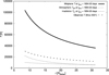 |
Fig. C.1 Same as Fig. 4 (top), but with Ck = 1.5 (opacity increases above the midplane) and A = 0. The increased isolation causes an increase in midplane temperatures. Teff and Tirr coincide well in the outer part of the disc. |
C.2 Solution 3: Irradiation
Considering the limited extent of the disc, it was to be checked that we weren’t crucially underestimating the influence of irradiation from the central star. In particular, the model does not include any edge-on irradiation. We thus artificially increased the temperature of the central star to T* = 50000 K and set the albedo to zero (A = 0). The effect on the temperature profile was negligible.
C.3 Solution 3: Vertical opacity profile
The Ck parameter (from Eq. (9) affects the vertical opacity profile. This parameter is typically set to 0.6 to account for a drop in opacity above the midplane in cool discs (Chrenko et al. 2017). The disc studied in this work may not be considered cool and hence the value of this parameter remains an open question. In principle, a single opacity law may govern the whole vertical opacity profile (Ck = 1). If an opacity law is inversely proportional to temperature, then in a disc where the temperature decreases with distance from the midplane, the opacity can theoretically grow. We tested the latter possibility by setting Ck = 1.5.
The temperature profiles plotted in Fig. C.1 show a substantial increase in midplane temperatures and a small increase in atmospheric temperatures (over 100000 K at the inner boundary and just under 40000 K at the outer boundary). The opacity increase in the vertical direction acts as an extra layer of isolation, that is the optical depth of the midplane increases. Teff and Tirr coincide well in the outer part of the disc, but both are lower than the observations. In the inner part of the disc, Teff is even higher than Tirr. This would break our assumption that the irradiation temperature serves as the thermodynamic limit to the atmospheric temperature.
The increase in temperature causes a thicker disc. The aspect ratio is thus in very good agreement with the observations.
The increase in temperature also implies an increase in viscosity (in Eq. 11 H ∝ √T and cs ∝ √T). The higher the viscosity, the more effective the transport of angular momentum and greater radial velocities; at the inner boundary velocities reach about 700 m s−1. A faster transport of matter is coupled with a decrease in surface densities (by ≈ 10%).
C.4 Solution 4: High α viscosity parameter
Using the analytical models, we demonstrated that a higher viscosity parameter α implies lower temperature profiles. Here, we present results for the limit case of α = 1.0 and also α = 1.5 (which is beyond the classical limit).
Shakura & Sunyaev (1973) introduced the parametrisation and reasons for the limit α ≤ 1.0, but the argumentation is based on a single source of viscosity. In fact, without a full theory of viscosity on the microscopic scale, this limit is not guaranteed. It is to be considered that several mechanisms of the angular momentum transfer may be present at once.
Even macroscopic phenomena may effectively add to the value of α, e.g., spiral waves induced by tidal forces propagating from the outer boundary inwards will travel at roughly the sound speed, which is slower than the orbital motion in the disc. This differential rotation leads to an angular momentum loss (Boffin 2008). This is possible when the 3:1 Lindblad resonance is located within the radial extent of the disc. According to Boffin (2008), this can be true for discs of q < 0.33. The β Lyr A disc (q = 0.223; Brož et al. 2021) is within the limit. The 1D simulations cannot resolve higher dimensions, but we found a reasonably good correspondence between the soundspeed timescale of adjusted observations and the binary period at the outer disc boundary. We take this as an additional argument that spiral waves may be present.
For both values of α, models stopped showing temporal evolution within a year and a half of the simulation time in all studied quantities.
High α means an effective angular momentum transport, combined with the fixed mass transfer implied an order of a magnitude lower surface densities (but still almost 10 times the observed profile) coupled with high radial velocities (up to 5000 ms−1).
The 10 (resp. 15) times increase in α resulted in a decrease by almost a half in the midplane temperatures. For the gas-pressure-dominated model with Kramers opacity, we derived the exponent over α to be  and
and  . The atmospheric temperatures Teff did not change significantly; this is coupled with the aspect ratio, which decreased to H/r ≈ 0.06.
C.5 Solution 5: Radiation pressure
In our initial considerations of the β Lyr A system, it was not clear how important the radiation pressure is for the dynamics of the system. The analytical models were mostly only consistent for the gas-pressure-dominated class and the numerical model used an ideal gas equation of state. We thus implemented a simple modification to the FARGO_THORIN code by Chrenko et al. (2017) to approximately account for additional pressure contribution due to radiation.
We expect that radiation pressure plays a role mainly in mechanical processes, hence we introduced two new parameters.
The definition of H holds for an ideal gas, but Montesinos et al. (2021) showed that when the radiation pressure is accounted for, the pressure scale height changes by a specific factor. They also introduced a numerical scheme to implicitly find this parameter. We introduced this factor into our model as a fixed parameter.
 (C.1)
where h denotes the dimensionless factor, H is the pressure scale height defined for an ideal gas, and Hr+p is the pressure scale height when radiation pressure is included.
(C.1)
where h denotes the dimensionless factor, H is the pressure scale height defined for an ideal gas, and Hr+p is the pressure scale height when radiation pressure is included.To approximate the role of the increased pressure in the dynamics, we introduced a second dimensionless factor p,
 (C.2)
(C.2)
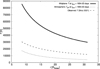 |
Fig. C.2 Same as Fig. 4, but for the modified numerical model accounting for the radiation pressure. The small addition to pressure causes a decrease in the midplane temperatures, but it does not affect the atmospheric temperatures. |
We included these two factors into the fluid equations of the numerical model. The value of p = 1.1 was estimated from pressure profiles generated by the gas-pressure-dominated analytical models and h = 1.75 is the approximate factor between the observed aspect ratio and the adjusted profile. The resulting temperature profile is shown in Fig. C.2.
We observe coupled phenomena, the aspect ratio increased in a consistent manner with the definition of the h factor (Eq. (C.1)). The expansion to a higher pressure scale height results in a slight decrease in the midplane temperatures, which intuitively follows from the ideal gas law. The atmospheric temperatures remained without significant changes due to a weakening of opacity in the vertical profile (i.e., lower optical depth, Eq. (9)). The surface density profile (as well as the radial velocities) remained the same; considering the increase in H, this implies the volumetric density decreased. The opacity (e.g. Kramers) is œ ρ, hence it also decreased. The increase in the radial pressure gradient also results in the disc being slightly more sub-Keplerian. Other studied quantities seem unaffected.
Appendix D Supplementary figures
Here, we present supplementary figures of profiles from our modified Shakura-Sunyaev models described in Sec. 6 and Appendix B.
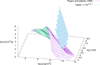 |
Fig. D.4 Same as Fig. 1, but where the parameters κ⊙, A, B were chosen so that the profiles from the modified Shakura-Sunyaev model, assuming Pg ≈ Pr, are consistent (i.e., without being constrained by Rogers & Iglesias 1992). |
All Tables
All Figures
|
Fig. 1 Rogers & Iglesias (1992) 2D opacity function (magenta) approximated by a plane (in a logarithmic plot) in the interval corresponding to Kramers’ opacity (cyan). |
| In the text | |
|
Fig. 2 Radial profiles of surface density (a), temperature (b), gas and radiation pressures (c), and aspect ratio of the β LyræA disc for a modified Shakura-Sunyaev model, which is gas-pressure-dominated and has Kramers’ opacity. The midplane temperatures and surface densities are significantly higher than the observed values. This also generates significantly higher pressure profiles. The observed aspect ratio is reached in hydrostatic equilibrium. |
| In the text | |
|
Fig. 3 Sketch of how presence of temperature inversion in vertical profile of disc could reconcile computed midplane temperature (Tmid) profile, the observed temperature profile and the calculated atmospheric Teff and irradiation Tirr profiles. |
| In the text | |
|
Fig. 4 Temperature, T(r) (top), surface density, Σ(r) (middle), and aspect ratio, H(r) (bottom), profiles of the time-dependent numerical model (from Table 3 with the Zhu et al. (2012) general opacity table). The midplane temperatures are significantly higher than the observations. The calculated atmospheric temperatures, Teff, and irradiation temperatures, Tirr, are of comparable magnitudes to the observations, but the correspondence between the temperature profiles is not satisfactory. Surface densities from the model are almost 100 times the observed value. The observed aspect ratio is reached in hydrostatic equilibrium. |
| In the text | |
|
Fig. C.1 Same as Fig. 4 (top), but with Ck = 1.5 (opacity increases above the midplane) and A = 0. The increased isolation causes an increase in midplane temperatures. Teff and Tirr coincide well in the outer part of the disc. |
| In the text | |
|
Fig. C.2 Same as Fig. 4, but for the modified numerical model accounting for the radiation pressure. The small addition to pressure causes a decrease in the midplane temperatures, but it does not affect the atmospheric temperatures. |
| In the text | |
 |
Fig. D.1 Same as Fig. 2, assuming "Ridge" opacity. |
| In the text | |
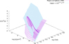 |
Fig. D.2 Same as Fig. 1 but suitable for regions with high temperatures. |
| In the text | |
 |
Fig. D.3 Same as Fig. 2, assuming Pg ≈ Pr and "Ridge" opacity. |
| In the text | |
|
Fig. D.4 Same as Fig. 1, but where the parameters κ⊙, A, B were chosen so that the profiles from the modified Shakura-Sunyaev model, assuming Pg ≈ Pr, are consistent (i.e., without being constrained by Rogers & Iglesias 1992). |
| In the text | |
 |
Fig. D.5 Same as Fig. 2, assuming Pg ≈ Pr and "Inverse problem" opacity. |
| In the text | |
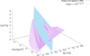 |
Fig. D.6 Same as Fig. 1, for "Extreme temperatures" opacity. |
| In the text | |
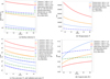 |
Fig. D.7 Same as Fig. 2, assuming Pg ≪ Pr and "Extreme temperatures" opacity. |
| In the text | |
Current usage metrics show cumulative count of Article Views (full-text article views including HTML views, PDF and ePub downloads, according to the available data) and Abstracts Views on Vision4Press platform.
Data correspond to usage on the plateform after 2015. The current usage metrics is available 48-96 hours after online publication and is updated daily on week days.
Initial download of the metrics may take a while.