| Issue |
A&A
Volume 704, December 2025
|
|
|---|---|---|
| Article Number | A13 | |
| Number of page(s) | 14 | |
| Section | Numerical methods and codes | |
| DOI | https://doi.org/10.1051/0004-6361/202553973 | |
| Published online | 01 December 2025 | |
Data-parallel methods for fast and deep detection of asteroids on the Umbrella platform: Near-real-time synthetic tracking algorithm for near-Earth objects
1
Astronomical Institute of the Romanian Academy,
5 Cuţitul de Argint,
040557
Bucharest,
Romania
2
Astroclubul Bucureşti,
Blvd Lascăr Catargiu 21,
10663
Bucharest,
Romania
XS
3
The University of Craiova,
Str. A. I. Cuza nr. 13,
200585
Craiova,
Romania
4
Isaac Newton Group (ING),
Apt. de correos 321,
38700
Santa Cruz de La Palma,
Canary Islands,
Spain
★ Corresponding author: This email address is being protected from spambots. You need JavaScript enabled to view it.
Received:
30
January
2025
Accepted:
18
August
2025
Abstract
Context. Further activities in detecting near-Earth asteroids (NEAs) using the blink method are hampered by the required size of the telescopes. Synthetic tracking (ST) is an effective solution, but the computational demands make operation difficult at survey data rates for fast moving objects.
Aims. We aim to show that, through efficient use of hardware, judicious pipeline design and choice of algorithms, ST at survey levels of data rates is possible even for objects with very fast apparent motion, such as NEAs.
Methods. We developed a GPU-accelerated ST pipeline, called synthetic tracking on Umbrella (STU), which targets real-time detection of fast NEAs through algorithms designed to make efficient use of data-parallel hardware. STU was developed as part of the Umbrella software suite, which we have expanded to provide an end-to-end data reduction pipeline.
Results. We demonstrate the capabilities of the STU pipeline to scan for moving objects faster than the acquisition rate at search radii of 10 arcseconds per minute, with good detection rates on several archival datasets without specific tuning.
Conclusions. Our investigation shows that ST is viable for large-scale surveys and that STU may perform such a role.
Key words: methods: data analysis / methods: numerical / techniques: image processing / minor planets, asteroids: general
© The Authors 2025
 Open Access article, published by EDP Sciences, under the terms of the Creative Commons Attribution License (https://creativecommons.org/licenses/by/4.0), which permits unrestricted use, distribution, and reproduction in any medium, provided the original work is properly cited.
This article is published in open access under the Subscribe to Open model. This email address is being protected from spambots. You need JavaScript enabled to view it. to support open access publication.
1 Introduction
Surveys that target the discovery of near-Earth objects (NEOs) are of significant importance in astronomy and for human life. While current surveys have discovered most NEOs larger than 1 km and have made significant progress in the detection of asteroids larger than 100 m, smaller objects tend to be discovered only during close flybys (e.g., Popescu et al. 2023).
Synthetic tracking (ST, also known as digital tracking: Allen et al. 2002) is a computational technique for detecting minor planets by combining multiple images of the same region of the sky while taking into account the apparent motion of a potential object across those images. By aligning and stacking the images along potential motion paths, synthetic tracking enhances the signal-to-noise ratio (S/N) of moving objects, which enables the detection of objects too faint to be detected in a single exposure.
With the exception of a few isolated cases (Yanagisawa et al. 2021), most minor planets have been found with the blink method, which involves comparing temporally separated images of the same region of the sky to detect objects with an apparent motion relative to the background sources. This can be done either using difference images, such as the software described by our previous paper (Stănescu & Văduvescu 2021), or using difference of detections, such as (Chambers et al. 2016), or other comparison techniques used by different moving object processing system implementations (such as Denneau et al. 2013). The main reason for the widespread use of blink is that methods such as ST are regarded as requiring vastly more computational power to analyze all possible object trajectories. This is particularly true for NEOs, since the apparent velocity of such objects is much higher than for other types of minor planets, even when using hardware acceleration (such as the works by Shao et al. 2014, Whidden et al. 2019, and Yanagisawa et al. 2021).
The blink method has several disadvantages compared to ST, due to its brightness requirements. At modern discovery magnitudes, V > 21 mag, due to multiple factors, new objects can be discovered using the blink method only with telescopes that have a large aperture (≫1 meters). First, skyglow becomes an important hindrance at these magnitudes. Even on dark nights (i.e., without the presence of the Moon in the night sky), for large telescopes or good cameras (and especially when both are combined), airglow becomes the dominant source of noise (larger than the noise from image sensors - readout or dark current). Furthermore, faster asteroids streak across the image and therefore cover more of the sky area with their source spread. As the flux of the noise through an area (of uncorrelated noise sources) increases with the square root of the area, the S/N of the streaking asteroids drops, even for algorithms that take streaking into account (by integrating along the potential motion vectors). As such, the blink method yields diminishing returns in the detection of new objects.
In comparison, ST directly addresses two of the above points: streaking (through integrating many short exposures) and the requirement for large telescopes (through its lower brightness requirements, as shown in Yanagisawa et al. (2005). Indirectly, however, it opens up the possibility of using other types of telescopes for this task, such as orbital ones (as proposed in Shao et al. (2014) or even stratospheric ones (which, due to the tracking difficulties are useful mostly for short exposures). As such, ST can easily detect new objects at much lower magnitudes compared to blink methods.
In this paper we show that a careful implementation of the ST concept can be sufficiently fast for real-time detection of fast NEOs (Section 3), present the software framework over which it was developed (Section 2), and discuss the early results from applying it to several archival datasets (Section 4). We finish with the discussion and conclusion of the results of our software implementation as well as their potential impact on the discovery of minor planets. The software implementation described in this paper is currently at technology readiness level (TRL) 41.
2 From raw images to astrometric reports: The Umbrella software suite
A complete system for automated search and reporting of asteroid discoveries involves many steps and software packages, starting from the firmware that controls the motors of the instrumentation (used in the mount, optical path, instrument auxiliaries, etc.) to the web interface for detection validation. Due to its large extent, to keep such a system maintainable, it needs to be split hierarchically into multiple components. To maintain high on-sky efficiency, each of these components, including the system itself, has to operate as pipelines. In such a system, top level components may be scheduling, motion and instrument control, data reduction, validation, and reporting.
The main focus of the EUROpean Near Earth Asteroids Research (EURONEAR)2 group (Vaduvescu et al. 2015) in the past few years has been the development of data reduction pipelines. We have approached this through activities including the first Umbrella version (Stănescu & Văduvescu 2021), the NEARBY online platform (Gorgan et al. 2019), the ParaSOL3 project (e.g. Popescu et al. 2023), and other derivative projects (e.g. Popescu et al. 2021; Kruk et al. 2022; Prodan et al. 2024). The data reduction pipelines developed in these projects extend from the handling the raw images acquired by the telescope, all the way to the human validation of detections, with plans to extend up to automated reporting of the astrometric positions to the Minor Planet Center database4 (MPC).
For this purpose, in the fourth version of the Umbrella software suite (continuing the work in Stănescu & Văduvescu 2021), we have implemented the concept of pipelines, which help developers build modular, user-configurable, and reusable data reduction and validation software components. The system architecture of a complete deployment of the Umbrella software suite is shown in Fig. 1.
2.1 Pipeline design
A pipeline is characterized by two critical parameters which capture the success of the process: the throughput and the latency.
In the case of asteroid detection, the former gives the survey coverage (i.e., how much of the sky can be observed and have the data processed in a given time), while the latter is the lower bound on the time it takes to get an alert to the community after the images of the asteroid have been acquired. The throughput can easily be scaled horizontally by adding more computational resources. However, the latency cannot be improved without improving the parallelism over individual fields and/or reducing the computational load of each field.
The importance of latency in the detection pipelines cannot be understated. If the detection results are not available in a timely manner, recovery from the same survey program in the same night may become unfeasible. For the fastest moving objects, this can lead to inability to recover on a follow-up observation if the object is not posted on the NEO confirmation page or otherwise shared with the community, which may happen for various reasons, including sufficient evidence of the detection being real.
The following terminology is used in this paper and by the Umbrella software suite:
The Pipeline elements are independent modules that may be loaded and assembled into a detection pipeline or a raw image reduction pipeline. Each element has a certain type (such as measurement element, filtering element, pairing element, reporting element, etc.), and can be plugged into a pipeline assembly into its corresponding role. Certain parts of the pipeline (such as measurement and filtering) allow applying multiple elements in succession.
A Pipeline host is an executable that can load the Umbrella pipeline elements, configure them according to a specified user configuration, and launch the pipeline over a set of inputs.
Raw science images (RAWSCI) are the science images as received from the image acquisition software as FITS files.
Bias, flat, and dark (BFD) are calibration images typically acquired at the beginning or at the end of the observing night. These images are used to correct for systematic errors of the imaging sensor.
Reduced science images (REDSCI) are the images obtained by applying the instrument-specific corrections, such as bias/dark current, flat field, bleeding/blooming (due to saturation from bright stars), crosstalk (due to amplifiers needed to read faster multichip cameras), and astrometric corrections (due to optical field distortions).
Below we describe the Webrella interface, the IPP, and the reporting module and formats. The STU module is described in Section 3, as it represents a key part of our software suite.
Finally, it should be mentioned that we have ported the reference blink pipeline from Stănescu & Văduvescu (2021) to the new Umbrella v4 pipelines. We have done so particularly to use the filtering methods developed as part of it. However, the effectiveness of ST has obsoleted the blink implementation for us and the blink pipeline is no longer maintained.
2.2 Image preprocessing pipeline (IPP)
We developed the IPP to apply the image corrections necessary for the instrumentation used, allowing us to use customized algorithms to achieve the REDSCI images with the best properties for the Umbrella detection pipelines. IPP includes corrections due to the sensor electronics (bias, dark, bad pixel) and instrumentation optics (flat field and optical distortion). Several additional scripts were implemented to correct the crosstalk and bleeding defects of the CCDs used in some of the telescopes.
Prior to the ParaSOL project, the IPP was an independent software package implemented on top of the Umbrella2 library. As part of the ParaSOL, we ported this software package to the pipeline system. The same steps, shown in Fig. 2, apply to both versions of the pipeline (legacy and new). However, the broader architecture view brought by this project has resulted in a refactoring of the way the steps are applied. Due to the target of real-time detection and reporting and the extremely fast resulting detection pipeline, the first step, of preprocessing the raw images, is a major contributor to the throughput and latency characteristics of the complete pipeline.
Starting from its original design, IPP works in a multithreaded approach over single images. As part of the latency focus of ParaSOL, the processing is now split into per-session operations and per-field operations. This improves the efficiency both in terms of throughput (the per-session data is computed only once in each session, i.e., observing night) and latency (only per-field data has to be computed once the telescope is in science mode, resulting in much shorter processing times).
To further reduce latency, the IPP was internally refactored to apply corrections to individual images as they are streamed into the system, rather than processing them in batches after all of them are received. This enables the synthetic tracking pipeline to begin processing almost immediately after receiving a single image, significantly minimizing delays. In fields with many images (a common scenario in ST), this approach reduces preprocessing time from minutes or even tens of minutes to just a few seconds.
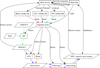 |
Fig. 1 Full system architecture. The various blocks (and their abbreviation) are described in the text. The methods to connect them are shown over each wire. Color coding of the data flows refers to the pipeline type, as all pipelines run as instances (processes) of the pipeline host: blue for STU, red for the reference blink pipeline, green for IPP. |
2.3 Webrella
We introduced the Webrella software package in Stănescu & Văduvescu (2021), where it provided a basic web interface to the blink pipeline. The quick growth of the Umbrella software, especially once the pipeline system has been developed, and the development of the IPP quickly obsoleted the version described before. However, the proven utility of the web interface for the detection pipelines, including the accessibility for users that no longer needed powerful hardware to validate detections, as well as the ease of collaboration, led us to develop a majorly overhauled version.
The new Webrella now is designed with the Umbrella v4 ecosystem in mind and allows interacting with the multiple pipelines supported by it. The interaction of Webrella with other components is shown in Fig. 1.
The organization of the interface has been improved to better handle re-reductions common when experimenting with different observing strategies, while keeping the convenient fastpath for well-established survey configurations. The final major overhaul was the development of a permissions system for the Webrella users, to enable survey administration over its web interface, while still allowing unprivileged reducer access, as well as scoped access to experiment data.
Moreover, the new web interface went through a major refresh, taking into account the major blockers in the previous interface, while keeping the strong points of its predecessor. A screenshot of the field validation interface is shown in Fig. 3. We preserved the characteristic light-weight resource usage and low-latency response time. We used JavaScript judiciously for several key features: keyboard navigation, previously available only in the desktop interface, automatic blinking of detection stamps, copying to the clipboard the detection report in 80-column format and stamp scale configuration.
On the server side, Webrella is now a FastCGI application5, instead of having an in-process web server. This allows it to be used with dedicated web server software that can handle tasks not requiring content generated on the fly. Moreover, for web servers that support such mechanisms, it allows using the autho-rizer role to gateway access to experiments based on the user’s permissions for the given experiment.
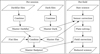 |
Fig. 2 IPP internal steps. |
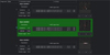 |
Fig. 3 Webrella interface, showcasing 2024 CW, a near-Earth asteroid discovered with STU at a 9.5 ”/min proper motion. Validated objects are highlighted in green. |
2.4 Reporting
For a detection pipeline to be useful, it must provide an effective and compatible output. The Umbrella v4 pipeline system has an internal, in-process representation of the detections. This allows for efficient processing within Umbrella, but it requires a reporting pipeline element to export it to a format that can be used by external systems.
The reporting pipeline element is designed to accept both graphical interfaces and batch operation. However, the format of the tests done as part of the ParaSOL project resulted in a focus on the batch operation, with the results of the detection pipeline stored in files on disk.
The following formats have been implemented in the Umbrella tooling: MPC 80-column, which although is a legacy format, it is still widely implemented in many asteroid detection tools. Our reporting tools output this format optionally from the batch reporting pipeline element and it is also available from the Webrella interface.
A comma separated values (CSV) file is used for storing the measured properties of the detection candidates. However, the focus here is to add these properties to the IPEF format described below.
The Astrometry Data Exchange Standard6 (ADES) is the new format for storing asteroid detection information as accepted by MPC. The Umbrella software suite support reading and writing in the XML format of ADES, although our framework is not fully compliant yet, with not all the required information being available when generating the report (for example, the astrometric and photometric calibration is done by the preprocessing pipeline, while the reports are created by the detection pipeline) and the ADES character limits not being implemented. The batch reporting pipeline element optionally outputs in this format and it is also the format available for download from Webrella.
The Inter-Pipeline Exchange Format (IPEF) is an internal format of our software. It is derived from ADES with the purpose of storing image and detection candidates properties and metadata for exchange between the image processing pipelines, detection pipelines, non-Umbrella candidate filters, as well as human validators and validation tools. This is the main format supported by the batch reporting pipeline. All other candidate report formats (80-column and ADES) are generated from it, both in the batch reporter and in the Webrella interface. It has been designed to be a companion format to ADES, where the latter is used to store and retrieve observation information from the MPC database, and the IPEF is used to carry detection information and metadata within asteroid detection software.
IPEF has currently been developed only to the degree that it can be used to carry information from the detection pipelines into Webrella; however there are future plans to further extend this format. First is to make IPEF bidirectionally convertible to/from the in-process Umbrella representation without significant loss of metadata, such that processing of detections can occur across process boundaries, allowing easy post-processing through Python scripts or for use in more advanced detection analysis tools running locally on the computers of astronomers, which can then be used to further refine the quality metrics for detection reporting. Another area of extension is on the preprocessing side, where it should carry the necessary image metadata for producing complete ADES reports from a detection pipeline or other downstream software (such as Webrella).
Due to the modular and extensible nature of the Umbrella pipelines, reporting the detections to the user involves an interplay of the detection element and the reporting element.
Common properties are passed through the detection representation, which are used to generate ADES and 80-column reports. However, even more information is extracted from the detection pipeline, which is made available through extensible reporting properties. These are used to pass user-facing measurements to the user interface layer. Moreover, the stamps shown to the user are also generated by STU, through a callback function. This is done such that interactive GUIs, with re-sizable stamp sizes, can be developed for STU. Multiple stamps are generated as a 2D list, over the different types of images (originals, masked, etc.) and sub-stacks. The design also supports sending plots as stamps (such as radial intensity plots), although this functionality has not be used yet.
The automated detection pipeline system is envisioned to provide the STU output to Webrella. For this reason, a reporter element called BatchReporter stores the results of the detection pipeline in IPEF format, as well as ADES XML and MPC 80-column converted from the IPEF representation. The extra information is stored in CSV files. Stamps are saved as PNG images, with the types of images, co-addition methods and size of the stamps configurable. The IPEF data, CSV files and stamps are read and displayed by the Webrella pipeline. The CSV data is made available in the list of properties of the web interface. The IPEF data is converted to MPC 80-column and displayed in the interface; upon validation, the selected detections are stored on disk on the server in the ADES format and downloaded to the reducer’s device at the same time. The stamps are shown on the right side of the detection line, with both dimensions accessible by keyboard navigation.
3 Synthetic tracking implementation
At the time Stănescu & Văduvescu (2021) was being published, our group began focusing on the synthetic tracking method. After considering and exploring the available options for achieving real-time synthetic tracking for surveys, the importance of co-addition modes and cache locality (see Chellappa et al. (2007) for explanations of the computing terminology) became clear to our group. To verify our hypotheses, we developed an initial prototype, which was a simplified version of the pipeline described in Fig. 4. This prototype became the cornerstone of the ParaSOL project, which aimed to develop the software suite, particularly the synthetic tracking implementation from TRL2 to TRL4. Therefore, the concepts presented in this paper are valid across its versions.
The following paragraphs and the pipeline diagram directly apply from v0.3, the first complete pipeline on the new module system, to v0.6. Newer STU versions apply equivalent operations, with different implementations and intermediate representations that improve runtime, but their detection performance is not yet characterized. For completeness, we mention that the results in this paper obtained primarily with v0.6.10, which is the latest release of the v0.6 series.
The following terms are used throughout the paper to explain the working of the pipeline:
Granularity is the sampling step of the trajectory space. STU is using pixels on the farthest image as its measure of granularity. For comparison, these are inversely proportional with the percentages from Tycho Tracker (Parrott 2020). A granularity of 1 px should correspond to a setting of 100% in Tycho and one of 2px to a setting of 50% in Tycho, although differences in the two implementations make this equivalence less exact.
Rays are hypothetical motion vectors, together with a starting point for the ray. In this paper, the term motion vector either implies a known starting point (in which case it is synonymous with a ray starting from the implicit pixel) or any starting point (such as when stacking whole images along a motion vector).
An isochrone is an image plane of equal time. Unless otherwise specified, it is an image or a set of images taken at the same time (i.e., for which the exposures are overlapping). We prefer this definition to highlight the intersection of a ray with an image, as well as cover the multisensor case, where multiple images may be used in generating a single isochrone of a macrotile. Finally, nonimage temporal planes are also useful for defining coordinate system references, such as the center isochrone below.
Macrotiles are image cubes (containing multiple isochrones, as described above) fed into the detection pipeline. In the STU versions described here, only a single macrotile may be processed from a set of input images (limiting the combined input image size to that of the GPU VRAM). Support for processing multiple macrotiles for a single field has been added since v0.7 of STU.
The center isochrone is a real (for odd isochrone count) or virtual (for even isochrone count) isochrone, at the median of the temporal axis of the macrotile. This is used as the reference for the ray coordinates. Note that STU assumes that the center isochrone occurs roughly in the middle between the first exposure in the macrotile and the last exposure in the macrotile. While deviations from this assumptions are expected to be functional, they may lead to suboptimal performance of the software, particularly in terms of increased runtime.
A visualization partially compatible (our ray origin is on the center isochrone and not on an edge one) with our definitions of ray, isochrone, and macrotile is presented by Whidden et al. (2019) (see Fig. 2 from page 9).
The STU pipeline is engineered from the ground up to attain the high processing throughput necessary to handle large volumes of data in real time (or near real time). Since the highest computational cost occurs in the brute force scanning phase, this step is surrounded by preprocessing and post-processing stages to hoist as much computation out of the scanning loop as possible. The stages of this pipeline are illustrated in Fig. 4.
In the preprocessing stage, the images are brought into the shape of a data cube that can be directly iterated over. This means resampling the images into a common coordinate system (such that the search occurs over pixel coordinates), as well as applying a mask that removes fixed sources. On the other side, the detection and post-processing part are designed around the concept of hypothesis rejection. This type of pipeline uses increasingly more expensive and effective filters to reject candidate detections from the list of motion vectors. This way, the brute force search can use an inexpensive quick check that is easily parallelizable over each pixel and motion vector.
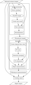 |
Fig. 4 STU internal pipeline stages. The image processing and the detection blocks are part of STU proper. The reduced science images are obtained with IPP or other preprocessing pipelines. The filtering and reporting is handled by other Umbrella modules. |
3.1 Image processing
On the preprocessing side, the first step is to evaluate the background level of the images, which is obtained from the first two statistic moments (mean and standard deviation) on small subblocks of the image, out of which the median values are used. The input images are then normalized them to a common level set in the pipeline configuration file, and co-added to obtain an image of the fixed sources. Co-addition is performed with a median averaging method, which leaves only faint residuals of the sufficiently fast moving objects (residuals which decrease with the number of input images, making this method perfect for deep synthetic tracking). The masking co-addition is necessary to mask faint stars that can be still picked up by the co-addition in the synthetic tracking although not bright enough to be detected in individual images. In particular, the signal to noise ratio is comparable to that of the detection method, which allows this method to be used in the blind as long as good enough astrometric data is available. The classic Umbrella blink blob detector (based on connected component of pixels above detection threshold, see Stănescu & Văduvescu 2021) is used to identify the bright fixed sources, which are directly and completely masked off. As discussed in Stănescu & Văduvescu (2021), completely masking off the bright sources eliminates the residuals from the slight differences in PSFs of the input images. Notably, for large scale surveys affording the use of a sufficiently deep (potentially locally-generated) reference star catalog, these steps may be bypassed in the future, using a list of known stars. To date, the usage patterns of STU have not suggested the need of such a method, for which reason no support for loading lists of known fixed objects has been implemented in STU up to now.
An optional high-pass filter is then used to remove large-scale patterns due to atmospheric effects (including halos from bright stars and Moon gradients). When the input data is of high quality and lacks such large-scale patterns, it is possible to turn off this filter, as it may introduce extra noise (due to it being generated from neighboring pixels), particularly on the edges of bright stars, where the plain mask shifts the background level lower than the local sky value, thus boosting the star edges. Except for such known minor inconveniences, the rolling median filter used for the removal of low-frequency patterns from the image has yielded satisfactory performance, comparable with the results given by astnoisechisel (Akhlaghi 2019).
The data is then resampled with nearest neighbor interpolation into a common World Coordinate System, currently chosen as that of the first image in the stack. Albeit imprecise, for nonphotometric usage this method has proven to be adequate while being much faster than the alternatives. Moreover, we intend to strongly recommend that input images should be already resampled to a common World Coordinate System from the preprocessing stage, leaving the internal resampling as a slower fallback option when the images cannot be prepared as such in advance.
3.2 Brute force scan
The core synthetic tracking operation is a brute-force scan over the whole data cube. The scan uses an associative score method (ASM), which is a highly effective generalization of the usual co-addition techniques used for synthetic tracking. The method used by STU has a low operation count per pixel, while maintaining robustness to noise and high selectivity, which are typical ASM advantages over its predecessors. These advantages and underlying concept of associative score methods as a generalization to the usual averaging co-additions will be described in an upcoming synthetic tracking review paper currently in preparation.
The scan is parallelized such that each workitem (one lane of the Single Instruction Multiple Data units of the processor) handles a group of 4x2 pixels (called microtile), while the motion vectors are scanned in a program loop. A further inner loop accumulates data over multiple images. The parallelization and loop order results in improved cache locality. The low computational cost method used by STU is normally dominated by the bandwidth required to access all the data once per each motion vector. For this reason, the much higher bandwidth between the execution units and the cache memory results in large speedups for STU. Furthermore, on newer versions of STU, the data accumulation is further sped up by small integer dot product instructions (which are typically used for quantized machine learning inference) on the accelerators that support them (including all modern AMD, Intel and ARM GPUs, but not nVidia). Currently, each microtile is split into two separate rays of 2x2 pixels; each of which is binned after sampling. The advantages of our approach compared to binning before sampling will be discussed in a future paper.
The scanned motion vectors are directly generated from the loop control variables, in a hollow cone pattern. There are two, configurable, velocity radii for the cone. First, there is an inner lower limit to avoid evaluating fixed sources that could yield scores higher than the desired target options. This is especially important for faint stars and stellar residue which remain unmasked (which is necessary to avoid threshold lowering of passing bright objects). The other is the maximum proper motion limit. The sampling step is also configurable, in terms of pixels on the farthest image, that is the distance in pixels between the intersection of consecutive motion vectors with the isochrone most distant from the center isochrone. In the ParaSOL project we customarily use a value of 0.99 pixels on the farthest image. This ensures that there are no gaps in the sampling, hitting each possible pixel within the motion cone.
The brute-force scan can be further sped up by a “third-ing” process, where the initial scan occurs only on a subset of the entire data, which would quickly eliminate implausible vectors before attempting to evaluate the score on the complete data cube. Limitations of the current implementation described below in this paper, particularly pixel hijacking have prevented the widespread use within the ParaSOL project. We expect this thirding process to become relevant after solutions are implemented to the described limitations and to be refined in the future into hybrid synthetic tracking with detection linking methods.
The result of the brute force scan is a list of the motion vectors. The current implementation provides at most one such motion vector for each input pixel, resulting in a highly selective filtering of the search space.
3.3 Hypothesis rejection
The individual motion vectors do not map, by themselves, directly into detections. Due to the PSF, a single object will be spread over multiple pixels and generally multiple microtiles. Moreover, the motion vectors from multiple microtiles of the same detection could be different. For this reason. the first stage following the brute force scan is the clustering of the motion vectors and pixels into detection blobs. The clustering is based on a connected component algorithm in the image space, keeping all motion vectors associated with the pixels in the detection. This is followed by scanning a stamp of the detection along each motion vector, using a trimmed mean co-addition. Each pixel of each stamp is evaluated together with its neighbors to determine the highest scoring ray of the detection. At this point, each individual detection corresponds to an individual candidate object, and filtering begins on the individual detection level.
A larger stamp (of configurable size) is then co-added along the ray on one or more sub-stacks (depending on the user supplied configuration) and the blink detector is applied to the stamp of each sub-stack to measure and extract the object. A set of filters is then applied based on the measured properties (such as full-width half maximum (FWHM), ellipticity, flux and magnitude, number of pixels, etc.) of the object and a tracklet is generated from the detections on the sub-stacks. There is a two-fold reason for doing so: first, the barycenter of the detection may be determined with potentially greater accuracy than the sampling step of the motion rays. Second, upon reporting to the Minor Planet Center, there is a requirement to provide independently estimated positions for each detection. By measuring the tracklet independently on each sub-stack, the software can provide such independent positions.
Finally, if the functionality is enabled, the detections are compared against the SkyBoT database. This step determines whether the objects are known or not.
4 Results
As a proof of concept for our methods, we present the results obtained from observations performed with three telescopes of varying apertures. Observations made with the 1.52 m Carlos Sánchez Telescope (TCS) were used to validate the detection of bright targets in a fully automatic manner with the default settings. The 0.25 m T025-BD4SB served as a test bench for generating various scenarios, including observations of extremely fast objects with different brightness levels relative to the detection limit. Here, we present the detection of a satellite. Finally, we utilized observations from the 2.54 m Isaac Newton Telescope, equipped with the old Wide Field Camera (WFC), to evaluate the performance of our methods on a noisy detector and to analyze potential errors and artifacts.
All these tests were focused on STU, while the IPP was only used for the INT data. The TCS and T025-BD4SB have their own automatic image processing pipelines for data preparation.
4.1 Hardware setup
Most of our tests, especially the early ones reported in this paper, were done on the ParaSOL1 computer. This computer had an AMD Ryzen 5700X CPU paired with 64GB RAM, which we upgraded in the second half of 2023 to a Ryzen 5950X with 128GB RAM. The other system specifications remained the same. The GPU used for ST is an AMD Radeon RX 6800 XT, with 16GB of VRAM. The software and the Ubuntu 22.04 LTS operating system have been installed to a Samsung SSD 980 1TB drive. The science data is stored on a RAID6 array of 6 Seagate IronWolf Pro 4TB hard drives, with an effective storage capacity of 16TB. The same RAID array was also used for intermediate data to minimize wear on the SSD until the RAM increase allowed us to use a tmpfs ramdrive to store the intermediate images.
A second PC (ParaSOL2) using the replaced Ryzen 5700X paired with 128GB and an AMD Radeon 7900XTX was installed in the second half of 2023. A similar storage setup was deployed using 6 Seagate Exos X16 16TB drives for an effective capacity of 64TB. Due to the release cadence of Ubuntu, the OpenCL stack for this GPU was not available on the Ubuntu OS at the time of the installation, requiring the use of a container, for which we chose ArchLinux. This made the setup more difficult to use.
For both PCs we used the ROCm OpenCL driver. To run the STU software, just as with any other Umbrella software, we used the latest mono7 package available at the time, which provides the implementation of the Common Language Runtime for running the Umbrella binaries.
4.2 The TCS data
We used the asteroid observations obtained with TCS as part of a survey conducted to characterize the color indexes of nearEarth objects (Popescu et al. 2021). The TCS is located at Teide Observatory (latitude: 28° 18′1.8″ N; longitude: 16° 30′ 39.2″ W; altitude: 2386.75 m).
It has a 1.52 m primary mirror mounted on an equatorial mount, with a focal ratio of f/13.8 in a Dall-Kirkham type configuration8. The survey employs the MuSCAT2 imaging instrument (an acronym for ‘a multicolor simultaneous camera for studying atmospheres of transiting exoplanets’) (Narita et al. 2019), which is installed at the Cassegrain focus of the telescope. A lens system reduces the focal length to a ratio of f/4.4.
This setup enables simultaneous photometric observations in four visible broad-band filters: g (400-550 nm), r (550-700 nm), i (700-820 nm), and zs (820-920 nm). Each of the four channels is equipped with an independently controllable CCD (chargecoupled device) camera (1024 × 1024 pixels) with a pixel scale of ~0.44″/px and a field of view (FoV) of 7.4 × 7.4 arcmin2. For testing the STU pipeline, we used only the data acquired with the r-band filter. The exposure duration was constrained by the tracking system. The telescope operates in equatorial tracking mode, but the aging mechanics of the instrument become unreliable for exposures exceeding 30-60 seconds, depending on the telescope’s orientation. Consequently, exposure times were generally limited to this range.
To test our data, we selected 242 fields acquired between May 28, 2018 and June 12 2022. Each field includes on average 112 images. These were already calibrated by the survey program. The preprocessing of the data consists of dark subtraction and flat-field correction. The calibration images were acquired at the beginning and end of the night. Then, the PHOTOMETRYPIPELINE (PP)-Mommert (2017), a software written in Python, performs the astrometric registration, aperture photometry, photometric calibration, and asteroid identification. PP uses the Astromatic suite9, namely SExtractor for source identification and aperture photometry (Bertin & Arnouts 1996), SCAMP for astrometric calibration (Bertin 2006), and SWarp for image regridding and co-addition (Bertin et al. 2002). The Gaia catalog (Gaia Collaboration 2018b; Gaia Collaboration 2018a) was used for astrometric registration. The PanSTARRS catalog (Tonry et al. 2012; Chambers et al. 2016) was used for photometric calibration of the data acquired with the Sloan filters.
The selected dataset includes asteroids with apparent motion lower than 5 arcsec/min (in compliance with the default setting for STU). Since the observations for this dataset were performed for photometric purposes, all asteroids are detectable in individual images. The distribution of the observed magnitudes (as reported by PP) and the apparent motion (as reported by the JPL Horizons10 system) are presented in Figs. 5 and 6.
All tests were conducted using the default settings for STU, including the apparent motion limit. The targeted asteroids were detected in all fields, and three positions were reported. The differences between the observed positions (as reported by STU) and the ephemerids (as computed using the JPL Horizons system) are shown in Fig. 7. The values are: (O - C)RA = −0.01 ± 0.36 arcsec and (O - C)Dec = +0.09 ± 0.37 arcsec. These results validate the detection of all bright targets using STU. Due to the small field of view of the TCS telescope, only the targeted NEA was within the field of view. Additionally, we note that for all these fields, no other candidates were reported by STU, indicating that no artifacts were introduced.
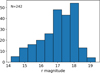 |
Fig. 5 Distribution of the apparent average r magnitude of the NEAs observed by TCS. |
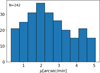 |
Fig. 6 Distribution of the apparent motions of NEAs observed by TCS. |
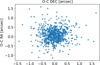 |
Fig. 7 Observed minus Computed (O-C) residuals for the 726 positions reported by STU for the 242 fields observed with TCS. |
4.3 Satellite detection using T025-BD4SB observations
The detection of very fast objects (with apparent motions on the order of hundreds or thousands of arcseconds per minute) presents a challenge for the ST algorithm due to the extremely high apparent motion, which requires a large search interval to detect the motion vector. Additionally, short exposure times must be used to limit the trail size, but this results in the detection of only a few stars in the field.
To test our STU algorithm in these cases, we observed several satellites using the T025-BD4SB telescope. The 0.25 m aperture T025-BD4SB telescope was built as a collaboration between professionals and amateurs, alongside amateur astronomers from Astroclubul Bucureşti. This telescope is a Newtonian design with a focal ratio of f/4, mounted on a robotized equatorial mount (Skywatcher EQ6-Pro). Images were captured with the QHY294M11 CMOS camera, operating in 11.7 megapixels mode, with a resolution of 0.956 arcsec/pixel.
A total of 36 observations were acquired on the evening of March 19, 2023, using the T025-BD4SB telescope. The exposure time was set to 1 second, and the satellite’s trail measured 35 pixels in length. After adjusting the configuration file, STU detected the satellite after approximately 3 minutes of computation, with 2 minutes and 32 seconds spent on the GPU. The velocity range used was 1800″/min-2200″/min with a granularity of 0.99px (corresponding to 1.54″/min), yielding a total of 4.8 trillion rays checked (average of ~4 × 10⁵ trajectories for each pixel), due to three quarters of the trajectories falling outside the field of view. The result is shown in Fig. 8.
Finally, because the object was bright, we checked and confirmed that the object can be detected with a subset of only 7 exposures. In this case, the 0.99 px granularity resulted in a sampling step of 8.6 ″/px, yielding an average of 0.54 trillion rays checked. In this case, the GPU runtime was merely 5 seconds.
4.4 Applications on the INT Image Archive
Nine fields were observed close to opposition or to the ecliptic (within 5 degrees) between 2019-2022 for ST projects using the 2.5 m Isaac Newton Telescope (INT) at Roque de los Muchachos Observatory (ORM) located atop La Palma island. Endowed at its f/3.3 prime focus with the Wide Field Camera (WFC) which consists of an L-shape mosaic of 4 2154 × 4200 (2048 × 4096 available optically) 13.5 μm CCDs (0.33 ″/px) which cover in total 0.25 sq.deg, the INT covers an etendue of 1.3 which is feasible for some deep survey works (discovery and recovery), and during the past decade we used this facility for such related projects (Văduvescu et al. 2013, 2015, 2018, 2021). In Table 1 we include the observing log, listing the field name, observing date and UT interval, telescope pointing (α and δ), the exposure time (E) and number of images taken in each field (N), the Solar elongation, airmass interval, average seeing (measured stellar FWHM), and the Moon phase (when the Moon was visible).
We used the ParaSOL Umbrella bundle v21 (STU v0.6.9) with its default configuration (i.e. we did not tune the parameters) to reduce the observed fields, detecting in total 184 valid moving sources, which include 142 known asteroids and other 42 unknown moving sources also cross-identified with the Tycho Tracker software.
We used IPP legacy version for image calibration (including astrometry) and STU for ST. We measured all known and unknown asteroids cross-correlated with Tycho detections, using the Pan-STARRS 1 catalog as the astrometric and photometric reference (due to the match of the INT Sloan r filter), which typically includes at least one hundred catalog stars in each reduced field of each CCD of the WFC.
According to the MPC database as of April 2024, queried by SkyBoT, there are 169 known asteroids within the nine observed fields covered by the WFC (one of which, due to its uncertainty, potentially outside the observed field). Following careful analysis of the individual reduced images, we counted 25 known asteroids invisible to blink (15% from the entire known sample), which actually represent an opportunity to test ST. From the subsample of 25 known asteroids invisible to blink technique, STU v0.6.9 detected ten targets and missed other 15. It also detected another two unknown asteroids, invisible to blink, which could be correlated with the Tycho Tracker.
Therefore, in its default configuration, STU detected 84% from all 169 known asteroids falling over the observed fields. From these 142 known asteroids detected, eight asteroids have only two positions (6% of the detected sample). Also, four asteroids (3%) had duplicate detection reports (resulting from disjoint clusters). Out of the other 27 known asteroids that could not be detected (16% of the entire known sample), some of them were lost in the noise caused by the known WFC CCD3 vignetted corner (where IPP masked the entire region due to increased noise), others due to slow motion (five objects had proper motions μ < 0.2,,) or due to involvement with fixed sources (stars). Finally, very bright targets (V magnitudes 15.8-18.3) were also not detected, most probably due to being filtered out as image artifacts. We expect that this detection ratio will be significantly improved once we deploy an automated tuning method. Reasons other than software processing for missed objects include faintness (expected apparent magnitudes V between 22.5-24.3), or/and fading due to light curves, weather and atmospheric factors (including Moon gradients) and instrumentation issues (such as slippage of the telescope tracking). As a point of reference, Tycho Tracker missed ten known asteroids (6%).
In Fig. 9 we plot the Observed minus Calculated (O-C) residuals for 407 synthetic tracking measurements of the 142 known asteroids detected by STU v0.6.9 in the nine INT archive fields. We found an average total residual of 0.19″ (0.02″ in α and 0.03″ in δ), and a total standard deviation of 0.12″, which is about one third of the size of a WFC pixel. We reported to the Minor Planet Center (MPC) all positions for all moving sources measured by STU, including all known asteroids plus the unknown detections matching Tycho findings.
In Fig. 10 we plot the histogram of all the apparent magnitudes of the 184 asteroids detected by STU in the nine fields, using relative photometry (Sloan r band matching the filter used for this INT survey) of the SDSS reference stars detected by IPP in the observed fields. An apparent limiting magnitude around R ~ 24.0 is visible, consistent with the INT SIGNAL12 predictions, giving the variable observing conditions of the 9 fields (R between 23.8-24.3 mag) and assuming signal to noise limit of 3. In comparison, using the classic blink detection with individual images taken in the same observing condition, the limiting magnitude was supposed to be only R ~ 21.9.
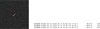 |
Fig. 8 Detection of a satellite using STU algorithm. The left side shows the STU output stamp obtained from stacking 12 exposures. The detection report in 80 columns format is shown on the right. |
Nine fields observed between 2019-2022 with the INT/WFC facility for synthetic tracking aims.
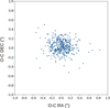 |
Fig. 9 Observed minus Calculated (O-C) residuals for 142 known asteroids detected in the nine INT observed fields. Root mean square residuals for 547 positions were detected and measured using STU, based on the Pan-STARRS DR1 catalog reference. An average O-C total residual of 0.19″ and a total standard deviation of 0.12″ were calculated. |
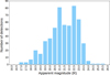 |
Fig. 10 Apparent magnitude (measured R values) for the 547 positions of the 184 asteroids detected in the nine INT observed fields, based on the photometric SDSS catalog reference. An apparent limiting magnitude cut around R ~ 24.0 is visible given the observed conditions of the nine amalgamated fields. |
4.5 Runtime
To compare the performance of this software across different workloads, we will use a metric named pixel processing rate (PPR). The PPR represents the number of image pixels visited (read from memory) in the brute force scanning stage over the time span needed to visit them. The associative scoring implementation used by STU allows it to visit each image only once per ray, hence the PPR scales linearly with the search space. Moreover, it is related more directly with the GPU specifications, such as memory bandwidth or floating operations per second (FLOPS) rating. The following equation makes the PPR definition precise:
 (1)
(1)
where C is the search space (number of pixels visited), W and H are the width and height of the data cube, J is the average number of trajectories tested per pixel (size of the search cone), and N is the number of images. Similarly υPPR is the pixel processing rate and τ is the time to scan all the pixels. As an example, we have recorded the detailed runtime information from running on the OPP3 field as well as the subset of the first 22 images. We chose the subset of 22 images due to a sharp discontinuity in the pixel processing rate (PPR) after this value. This suggests that 22 images better fit the GPU cache, especially since the pixel processing rate for the full OPP3 field is nearly identical with the
PPR at 23 images. In both cases, we ran with a search cone with a maximum proper speed of 20 ″/min. Due to the large maximum proper speed compared to the image size, many trajectories fall outside the data cube and are not tested. In both cases the granularity was set to 0.99px∕s. However, the sampling steps are different, due to the time between the first and last images being different between the full field and the subset.
For the following examples, we provide the values of W and H for the data cube (which can be different from the individual image sizes) from the compiler arguments of the GPU code. The maximum trajectories per pixel is computed from the sampling step and the search cone radius, both also passed as compiler arguments. For C, STU reports the value by computing it from WHJ, the total number of trajectories actually scanned, and N. The total number of trajectories scanned is measured on the GPU (for performance reasons implemented with parallel private counters on each workitem, which are atomically summed into a global counter once the workitem finished processing the microtile).
On the full OPP3 field, with N = 30, W = 4240, H = 2224, we have C = 3.9 × 10¹⁴, giving an average J = 1.38 × 10⁶, out of 2.6 × 10⁶ maximum trajectories per pixel. With a τ = 419 s (7 minutes brute force scan, 8.1 minutes complete STU execution), we have a PPR of 931 Gpx/s.
On the first 22 images of OPP3, we have N = 22, W = 4240, H = 2224, and C = 1.87 × 10¹⁴, giving an average J = 9.01 × 10⁵ out of 1.4 × 10⁶ maximum trajectories per pixel. With a τ = 132 s (2.2 minutes brute force scan, 3.5 minutes complete STU execution), we have a PPR of 1412 Gpx/s.
To put these results into perspective, this GPU has 512 GB /s bandwidth to the VRAM, and a 20 TFLOPS rating (it can execute ten trillion instructions per second). These results also demonstrate the ability of STU to exploit cache locality, as an implementation that co-adds the images would under no circumstances be able to exceed 512 Gpx/s, the maximum bandwidth to the VRAM of the card used, when co-adding 8-bit images. By comparison, STU achieves twice to thrice this bandwidth, at an equivalent of 7-11 instructions per pixel.
4.6 Limitations of our software
Among the limitations of the method used in STU, we have observed two forms of detection hijacking, both different from the ‘detection hijacking’ concept introduced in our previous blink pipeline (see Stănescu & Văduvescu 2021). Nonetheless, all three types result in losing a true positive from overlapping false positives.
Pixel hijacking: one of the detection hijacking modes observed in STU is pixel hijacking. Due to the output of the first stage containing at most one motion vector per pixel, whenever many bright image artifacts appear in the raw images, or, in the case of very low S/N of the true positives, even noise, which may line up and cross the same center isochrone as a real detection, then these artifacts may end up as the highest-scoring vector for the given pixel on the center isochrone. In a quick investigation of the loss of a few true positives when activating the thirding mode of STU, this has been identified as the most common cause, followed closely by low visibility on the central images (due to crossing image gaps, from either sensor gaps or areas with dense masks of image artifacts).
Notably, pixel hijacking demonstrates the data dredging effects of the ST technique. If a true positive is suppressed by false positives, then a similar set of false positives would be present in the output of the stage. By using other correlating information, false positives will be suppressed, however the correlating information typically loses its information value to the latter validation steps (especially human validators), as the filtered results cherry-pick the candidates which already fit the expected profiles of real detections.
This way we would like to express support for opinions of caution in the reporting of candidates from ST - some of the criteria human validators have been using to tell apart false positives from real detections may already have been used in the reduction pipelines and the confidence of detecting a real object may in practice be lower than expected by validators not trained and knowledgeable in the filtering stages of the detection pipelines.
Cluster hijacking: our software is also susceptible to hijacking in the second (clustering) stage leading to either candidate elimination in the third stage or third stage false positive hijacking. This occurs by including the real objects inside large false positive clusters. In such cases, a true positive may be suppressed by the neighboring false positives, especially in areas of high background variability, where large clusters of false positives may appear.
Catastrophic percolation: Percolation is the most obvious and an extreme kind of cluster hijacking. Unlike the regular cluster hijacking which occurs on a small scale, when operating the software close to the noise floor of the method (using detection thresholds that allow a large percentage of noise to exit the brute force stage), a phase transition occurs where clusters ’precipitate’ from the random noise in large amounts and sizes. As the detection threshold is lowered, clusters merge and true positives decrease up to a catastrophic loss of detections.
This is an effect of site percolation in the clustering stage. As the detection probability of random noise on a single pixel approaches and exceeds the critical site percolation probability of the square lattice (approximately p ≃ 0.593, according to Akhunzhanov et al. 2022), random noise starts to cluster quickly on large scales (size distribution becomes subexponential, approaching a power law with the Fisher exponent of τ = 187/91), and therefore begins cluster hijacking all across the macrotile. This has been observed when optimizing parameters over recently acquired data from the telescope installed by the Korea Astronomy and Space Science Institute (KASI) at the Cerro Tololo Inter-American Observatory; the original analysis is presented in Văduvescu et al. (2025). At detection thresholds under 3 standard deviations of the co-added image, we have often observed one cluster larger than half the size of the entire image.
Limiting magnitude: STU has an effective detecting limit ~ 0.5 magnitudes above the limit of the Tycho Tracker software. This is due to the percolation limitation above and the lack of a prioritization scoring method for the human validation, with our usual detection settings.
5 Discussion and conclusion
We have implemented and proven the operation of a real-time ST pipeline for the detection of near-Earth asteroids. The results from the early phases of the development also prove its detection capabilities, especially on datasets where preprocessing was effective at eliminating the image artifacts. The lower detection rates on the datasets with lots of sensor artifacts (such as INT above, or the telescopes of the Korean Microlensing Telescope network) highlight the need for improved tuning capabilities for our software in order to reach mission grade technology readiness levels.
Nonetheless, even at the current development stage, the ability of STU to scan for objects moving at much faster rates has yielded several independent discoveries that would have been difficult to achieve with other methods. For example, 2023 XA3 was detected at 7.8 arcsec/min in the 2° × 2° field of view of the KASI telescope. This object and other results from applying STU to live mini-surveys are presented in Văduvescu et al. (2025). The degree to which such a fast implementation can impact the capabilities for minor planet discovery are discussed in the next paragraph, followed by the steps we identified that we need to take in order to bring our implementation to the maturity needed to achieve the impact described. Some of these steps have already been implemented, and are in the testing phases; the results will be available in an upcoming paper, including a more detailed analysis of runtime, energy draw, and other factors of interest over a wider variety of hardware.
5.1 Implications of fast synthetic tracking
Our opinion is that a fast ST implementation is capable of fundamentally changing the approach to detecting new, fainter, asteroids. We expect that once such a method becomes widely available, ST will rapidly and completely replace the classical blink method.
On a short timescale, we expect to see shallow deployments (namely ST using few, often less than ten exposures) replacing blink pipelines in existing large surveys, driven by the need to scan deeper than the long-reached limits of the blink method of the telescope. These shallow deployments are able to reuse the instrumentation designed for blink (which may not have particularly fast readout speeds) to go deeper than previously possible. In parallel, we expect an explosive growth in proposals for new surveys using dedicated hardware (many small telescopes with very large etendue, as well as fast sensors). This should not be a surprise, as there are already very effective dedicated ST surveys, such as Maury - Attard - Parrot (MAP)13, which have already demonstrated the capabilities of this method, by discovering in just a few years hundreds of NEAs using a few RASA 11″ telescopes and the Tycho Tracker software developed inhouse. Finally, as the benefits of this method become obvious, there will be extensive focus on ramping up the know-how of the community on the practical aspects of deploying ST surveys.
On longer timescales, we expect batteries of smaller telescopes to become the norm for asteroid surveys, due to their much lower cost than total etendue equivalent large telescopes, given a limiting magnitude and sky coverage targets. As more surveys will use ST, even large mirror telescopes will have difficulty discovering faint asteroids compared to massive arrays of small telescopes, if these large telescopes will keep using the blink method. For this reason, we expect that all large-scale surveys will end up using ST.
For the extremely wide fields allowed by massive telescope batteries (which can cover almost the whole sky), the next major bottleneck will be the maximum integration time allowed by the method, especially when considering the fastest moving objects, such as those passing within a few Lunar distances or even inside the Moon’s orbit. Similarly, dredging the list of potential objects for cross-night confirmations can push the minimum S/N for valid detections even lower. For these, we expect the extension of the current ST methods with blink techniques of pairing sparse detections, which would allow the total integration time to be extended far beyond the current pure ST approaches.
However, the largest impact might not even be on groundbased surveys. This method has the potential to unlock niche approaches to detecting asteroids, through the use of balloon-borne and small space telescopes. Both these approaches alleviate or remove the effects of the atmosphere, which currently are the main roadblocks in detecting fainter objects. In particular, on space telescopes, where weight is typically far more expensive than the complexity of the optics, it is far more convenient to use a small mirror with a large field of view optical system. For these systems, ST is a good fit, trading faintness for a narrower scan area, which allows the detection of asteroids at a distance. A side advantage to such free-floating telescopes is the method’s innate image stabilization compatibility (as it can work with very short exposures directly and does not necessarily require a separate recombination step as digital stabilization does or complex hardware for optical stabilization). These advantages are particularly valuable when considering objects approaching Earth from the side illuminated by the Sun, which require space-based telescopes to detect ahead of impact, such as the proposed Near-Earth Object Mission in the Infrared (Licandro et al. 2024). Finally, the increase in detection capabilities from the use of high-speed ST will expand the database of known NEAs, some of which are far more easily accessible for space missions, including those of an industrial nature (for example asteroid mining).
On a side note, we expect that ST will lead the way to other computationally intense operations being accelerated by fast programmable hardware. One notable such example is the image preprocessing step, since applying dark and flat-field photometry corrections is a massively parallel problem. Similarly, thanks to highly efficient index structures of plate solving software (such as Astrometry.net), one major cost of plate solving is the (robust) detection of stars and their measurement, which can also be parallelized to a large degree.
5.2 Future steps
Thanks to the many observing runs on which we achieved realtime or near real-time data reduction, we have discovered several practical bottlenecks not initially envisioned in the project. The biggest issue we have yet to work on is the quality control of our intermediate steps, particularly the REDSCI images. Having a human check the REDSCI images introduces significant delay and makes automating pipelines difficult. For quick cadence surveys, having a high image throughput and/or real-time reporting, where the latency introduced by checking the intermediate images and synchronizing with the status of the pipelines, checking these intermediate results should be automated. Another related issue is the difficulty of adjusting parameters on the fly if the outputs are wrong. This can easily happen due to variance of the sky conditions (cirrus or variable amount of clouds, seeing, background gradients due to Moon, etc). For example, if the default parameters for Astrometry.net (Lang et al. 2010) fail (due to differences in the number of detected stars, for example), different ones are needed, and this change should happen as soon as possible. Similarly, if the PSF changes significantly, tuning the detection parameters may be necessary to keep detecting objects or drop false positives. For these, the degree of image measurement and self-tuning needs to be improved. Moreover, existing tuning tools (such as the Object Tracer in STU) need improved infrastructure, such as the ability to automatically retrieve known objects in the field of view, identify the detection blockers, and automatically identify tuned parameters that would enable the detection of said objects.
Also on the tuning side, we plan to improve our parameter tuning setup based on the accumulated database of known valid and invalid objects. This again requires more infrastructure around STU’s Object Tracer and improved usability. Currently, the Object Tracer is just a logging tool that enables some logging logic in a certain image region and search cone. For this and the previous purpose, it also needs to be able to output structured data, such as the thresholds that need to be set for a certain object to pass. Moreover, to improve the speed of the tuning, it needs the ability to trace multiple objects.
In the shorter term, we implemented the re-tiling of large mosaic sensors (making it possible to run ST on images larger than the VRAM limits of the GPUs) and we re-wrote our pipeline stages to improve the runtime, including merging some GPU operations, changing algorithms, and moving a large number of operations to the GPU, which are available starting with STU v0.7.0. These, together with an improved measurement stage, will be presented in an upcoming paper.
In the longer term, we plan to improve our IPEF specification and make it public. In particular, we plan to better define the REDSCI-associated information, including information on the astrometric and photometric calibration, which is needed for the ADES conformance of the detection pipelines output reports. We also plan to use digest2 (Keys et al. 2019 and Veres et al. 2023) and Find_Orb14 to highlight potentially interesting objects.
Based on the observing runs and our reducers’ experience with Tycho Tracker, several inconveniences were identified with the Web GUI, such as the inability to re-stack with larger window sizes. The lack of the desktop GUI for STU (which we have yet to adapt from the old blink pipeline), which would have solved the previous problem and slightly increased responsiveness, has also been raised several times by our reducers. Finally, a point was raised internally on using the pipeline directly from Python, bypassing the use of the executable pipeline host. This was demonstrated to be possible although cumbersome, and was made difficult by the lack of convenient documentation formats. For this, we plan to add doxygen to the CI scripts to export the documentation in all the pipelines and not just the core library (umbrella2).
Acknowledgements
The work for this article was supported by a grant of the Romanian National Authority for Scientific Research (UEFISCDI), project number PN-III-P2-2.1-PED-2021-3625 (PI: Marcel Popescu), contract number 685PED registered on 21/06/2022.
References
- Akhlaghi, M. 2019, arXiv e-prints [arXiv:1909.11230] [Google Scholar]
- Akhunzhanov, R. K., Eserkepov, A. V., & Tarasevich, Y. Y. 2022, J. Phys. Math. Theor., 55, 204004 [Google Scholar]
- Allen, R. L., Bernstein, G. M., & Malhotra, R. 2002, AJ, 124, 2949 [Google Scholar]
- Bertin, E. 2006, ASP Conf. Ser., 351, 112 [NASA ADS] [Google Scholar]
- Bertin, E., & Arnouts, S. 1996, A&AS, 117, 393 [NASA ADS] [CrossRef] [EDP Sciences] [Google Scholar]
- Bertin, E., Mellier, Y., Radovich, M., et al. 2002, ASP Conf. Ser., 281, 228 [Google Scholar]
- Chambers, K. C., Magnier, E. A., Metcalfe, N., et al. 2016, arXiv e-prints [arXiv:1612.05560] [Google Scholar]
- Chellappa, S., Franchetti, F., & Püschel, M. 2007, How to Write Fast Numerical Code: A Small Introduction (Berlin, Heidelberg: Springer-Verlag), 196 [Google Scholar]
- Denneau, L., Jedicke, R., Grav, T., et al. 2013, PASP, 125, 357 [NASA ADS] [CrossRef] [Google Scholar]
- Gaia Collaboration 2018a, VizieR Online Data Catalog: Gaia DR2 [Google Scholar]
- Gaia Collaboration, 2018, VizieR On-line Data Catalog: I/345 [Google Scholar]
- Gaia Collaboration (Brown, A. G. A., et al.) 2018b, A&A, 616, A1 [NASA ADS] [CrossRef] [EDP Sciences] [Google Scholar]
- Gorgan, D., Văduvescu, O., Stefanut, T., et al. 2019, arXiv e-prints [arXiv:1903.03479] [Google Scholar]
- Keys, S., Veres, P., Payne, M. J., et al. 2019, PASP, 131, 064501 [Google Scholar]
- Kruk, S., García Martín, P., Popescu, M., et al. 2022, A&A, 661, A85 [NASA ADS] [CrossRef] [EDP Sciences] [Google Scholar]
- Lang, D., Hogg, D. W., Mierle, K., Blanton, M., & Roweis, S. 2010, AJ, 139, 1782 [Google Scholar]
- Licandro, J., Conversi, L., Delbo, M., et al. 2024, in European Planetary Science Congress, EPSC2024-882 [Google Scholar]
- Mommert, M. 2017, Astron. Comp., 18, 47 [Google Scholar]
- Narita, N., Fukui, A., Kusakabe, N., et al. 2019, J. Astron. Teles. Instrum. Syst., 5, 015001 [Google Scholar]
- Parrott, D. 2020, J. Am. Assoc. Variab. Star Observ., 48, 262 [Google Scholar]
- Popescu, M., de León, J., Licandro, J., et al. 2021, in European Planetary Science Congress, EPSC2021-820 [Google Scholar]
- Popescu, M. M., Văduvescu, O., de León, J., et al. 2023, A&A, 676, A126 [NASA ADS] [CrossRef] [EDP Sciences] [Google Scholar]
- Prodan, G. P., Popescu, M., Licandro, J., et al. 2024, MNRAS, 529, 3521 [Google Scholar]
- Shao, M., Nemati, B., Zhai, C., et al. 2014, ApJ, 782, 1 [NASA ADS] [CrossRef] [Google Scholar]
- Stănescu, M., & Văduvescu, O. 2021, Astron. Comp., 35, 100453 [Google Scholar]
- Tonry, J. L., Stubbs, C. W., Lykke, K. R., et al. 2012, ApJ, 750, 99 [Google Scholar]
- Văduvescu, O., Birlan, M., Tudorica, A., et al. 2013, Planet. Space Sci., 85, 299 [Google Scholar]
- Văduvescu, O., Hudin, L., Tudor, V., et al. 2015, MNRAS, 449, 1614 [Google Scholar]
- Văduvescu, O., Hudin, L., Mocnik, T., et al. 2018, A&A, 609, A105 [NASA ADS] [CrossRef] [EDP Sciences] [Google Scholar]
- Văduvescu, O., Gorgan, D., Copandean, D., et al. 2021, New A, 88, 101600 [Google Scholar]
- Văduvescu, O., Stănescu, M., Popescu, M., et al. 2025, New Astron., 119, 102410 [Google Scholar]
- Veres, P., Cloete, R., Weryk, R., Loeb, A., & Payne, M. J. 2023, PASP, 135, 104505 [Google Scholar]
- Whidden, P. J., Bryce Kalmbach, J., Connolly, A. J., et al. 2019, AJ, 157, 119 [NASA ADS] [CrossRef] [Google Scholar]
- Yanagisawa, T., Nakajima, A., Kadota, K.-i., et al. 2005, PASJ, 57, 399 [Google Scholar]
- Yanagisawa, T., Kamiya, K., & Kurosaki, H. 2021, PASJ, 73, 519 [NASA ADS] [CrossRef] [Google Scholar]
See https://www.nasa.gov/pdf/458490main_TRL_Definitions.pdf for the definitions of each TRL level.
All Tables
Nine fields observed between 2019-2022 with the INT/WFC facility for synthetic tracking aims.
All Figures
|
Fig. 1 Full system architecture. The various blocks (and their abbreviation) are described in the text. The methods to connect them are shown over each wire. Color coding of the data flows refers to the pipeline type, as all pipelines run as instances (processes) of the pipeline host: blue for STU, red for the reference blink pipeline, green for IPP. |
| In the text | |
|
Fig. 2 IPP internal steps. |
| In the text | |
|
Fig. 3 Webrella interface, showcasing 2024 CW, a near-Earth asteroid discovered with STU at a 9.5 ”/min proper motion. Validated objects are highlighted in green. |
| In the text | |
|
Fig. 4 STU internal pipeline stages. The image processing and the detection blocks are part of STU proper. The reduced science images are obtained with IPP or other preprocessing pipelines. The filtering and reporting is handled by other Umbrella modules. |
| In the text | |
|
Fig. 5 Distribution of the apparent average r magnitude of the NEAs observed by TCS. |
| In the text | |
|
Fig. 6 Distribution of the apparent motions of NEAs observed by TCS. |
| In the text | |
|
Fig. 7 Observed minus Computed (O-C) residuals for the 726 positions reported by STU for the 242 fields observed with TCS. |
| In the text | |
|
Fig. 8 Detection of a satellite using STU algorithm. The left side shows the STU output stamp obtained from stacking 12 exposures. The detection report in 80 columns format is shown on the right. |
| In the text | |
|
Fig. 9 Observed minus Calculated (O-C) residuals for 142 known asteroids detected in the nine INT observed fields. Root mean square residuals for 547 positions were detected and measured using STU, based on the Pan-STARRS DR1 catalog reference. An average O-C total residual of 0.19″ and a total standard deviation of 0.12″ were calculated. |
| In the text | |
|
Fig. 10 Apparent magnitude (measured R values) for the 547 positions of the 184 asteroids detected in the nine INT observed fields, based on the photometric SDSS catalog reference. An apparent limiting magnitude cut around R ~ 24.0 is visible given the observed conditions of the nine amalgamated fields. |
| In the text | |
Current usage metrics show cumulative count of Article Views (full-text article views including HTML views, PDF and ePub downloads, according to the available data) and Abstracts Views on Vision4Press platform.
Data correspond to usage on the plateform after 2015. The current usage metrics is available 48-96 hours after online publication and is updated daily on week days.
Initial download of the metrics may take a while.