| Issue |
A&A
Volume 704, December 2025
|
|
|---|---|---|
| Article Number | A96 | |
| Number of page(s) | 21 | |
| Section | Stellar atmospheres | |
| DOI | https://doi.org/10.1051/0004-6361/202554071 | |
| Published online | 09 December 2025 | |
Investigating episodic mass loss in evolved massive stars
IV. Comprehensive analysis of dusty red supergiants in NGC 6822, IC 10, and WLM
1
IAASARS, National Observatory of Athens,
15326
Penteli,
Greece
2
National and Kapodistrian University of Athens, Department of Physics, Panepistimiopolis,
15784
Zografos,
Greece
3
Institute of Astrophysics FORTH,
71110
Heraklion,
Greece
4
Instituto de Astrofísica de Canarias, Avenida Vía Láctea,
38205
La Laguna, Tenerife,
Spain
5
Grantecan S. A., Centro de Astrofísica de La Palma, Cuesta de San José,
38712
Breña Baja, La Palma,
Spain
6
Centro de Astrobiología, CSIC-INTA,
Ctra. de Torrejón a Ajalvir km 4,
28850
Torrejón de Ardoz, Madrid,
Spain
★ Corresponding author: This email address is being protected from spambots. You need JavaScript enabled to view it.
Received:
7
February
2025
Accepted:
17
October
2025
Abstract
Mass loss shapes the fate of massive stars; however, the physical mechanism causing it remains uncertain. We present a comprehensive analysis of seven red supergiants, for which we searched evidence of episodic mass loss, in three low-metallicity galaxies: NGC 6822, IC 10, and WLM. Initially, the spectral classification of their optical spectra was refined and compared to previous reported classifications, finding four sources that display spectral variability. We derived the physical properties of five of them using the MARCS atmospheric models corrected for nonlocal thermal equilibrium effects to measure stellar properties from our new near-infrared spectra, such as the effective temperature, surface gravity, metallicity, and microturbulent velocity. Additional empirical and theoretical methods were employed to calculate effective temperatures, finding consistent results. We constructed optical and infrared light curves, discovering two targets in NGC 6822 with photometric variability between 1 and 2.5 mag in amplitude in r and ~0.5 mag in the mid-infrared. Furthermore, we discovered a candidate-dimming event in one of these sources. Periods for three red supergiants were determined using epoch photometry, which were consistent with the empirical estimations from literature period-luminosity relations. Our comprehensive analysis of all the available data for each target provides evidence for episodic mass loss in four red supergiants.
Key words: stars: atmospheres / stars: fundamental parameters / stars: late-type / stars: massive / stars: mass-loss / supergiants
© The Authors 2025
 Open Access article, published by EDP Sciences, under the terms of the Creative Commons Attribution License (https://creativecommons.org/licenses/by/4.0), which permits unrestricted use, distribution, and reproduction in any medium, provided the original work is properly cited.
This article is published in open access under the Subscribe to Open model. This email address is being protected from spambots. You need JavaScript enabled to view it. to support open access publication.
1 Introduction
Massive stars, which are stars with masses M ≥ 8 M⊙, are powerful engines that drive the evolution of their host galaxies with their feedback (e.g., McCray & Kafatos 1987). At the end of their lifetime, they explode as a supernova or implode directly to a black hole (Heger et al. 2003). Most of them evolve through the red supergiant (RSG) phase (Levesque 2017), during which they undergo both long timescale mass-losing processes, such as stationary winds (e.g., Beasor et al. 2020; Antoniadis et al. 2024), as well as short timescale events, such as eruptive mass loss (Smith 2014; Humphreys & Jones 2022). These processes and their potential metallicity dependence remain poorly understood (e.g., Decin 2021), although they determine how much of the H envelope a star ultimately sheds and therefore its finale (e.g., Smith et al. 2011; Georgy 2012).
To understand the winds of RSGs and their driving mechanism, one needs to model their atmospheres. However, this task poses a significant challenge, as their structure is very complex due to the outer layers being convective (Freytag et al. 2002; Ludwig et al. 2009), exhibiting granulation (Chiavassa et al. 2009), as well as strong turbulence (e.g., Josselin & Plez 2007; Ohnaka et al. 2017) – phenomena induced by convection (Freytag et al. 2012). To study these effects, 3D magnetohydrodynamical and radiative hydrodynamics simulations are needed (e.g., Meyer et al. 2021; Goldberg et al. 2022, respectively). In addition, large-scale convection in the stellar interior and self-excited pulsations result in atmospheric dynamics with strong radiative shock waves (Freytag et al. 2024). These extreme atmospheric conditions make the extraction of their physical parameters, and in particular the effective temperature (Teff), quite difficult, while the luminosity (L) can be measured by spectral energy distribution (SED) fitting. The stellar radius (R) is derived from the Stefan-Boltzmann law.
Various approaches are used to determine the RSG Teff; however, some produce discrepant results. The most commonly employed method is to model the titanium oxide (TiO) bands in their optical spectra, as TiO bands are sensitive to Teff and optical spectra are readily available. However, modeling TiO bands yields systematically lower Teff (by ~300 K) than other methods (e.g., SED fitting; Davies et al. 2013) because these lines form in the outer atmospheric layers of the RSGs, where the optical depth (τ) is less than one, probing lower temperature regions. Furthermore, TiO bands are affected by metallicity and mass loss, which cause them to appear deeper (Davies & Plez 2021). The combined effect of Teff, metallicity, and mass loss on the strength of the TiO bands cannot be disentangled in the optical.
An alternative method to determine the Teff of RSGs is modeling atomic lines in their J-band spectra. The method produces more accurate Teff results than the modeling of the TiO bands because it uses lines that form near the stellar continuum region (τ ~ 1). This technique was introduced by Davies et al. (2010), originally aiming to derive metallicities of RSGs by exploiting the fact that their SED peaks in the near-infrared (near-IR), which is applicable even at large distances (Evans et al. 2011; Lardo et al. 2015). It comprises of fitting Fe, Si, Ti, and Mg absorption lines present in the observed spectra with synthetic spectra to estimate stellar parameters. Davies et al. (2015) demonstrated the strong Teff sensitivity of the J-band modeling method and derived error bars of ~50 K, which are comparable with those extracted using the SED fitting technique for the same dataset. This is the most accurate method to calculate RSG Teff (Davies et al. 2013); however, it requires spectroscopic data covering a wide wavelength range. In the absence of J-band spectroscopy, empirical or theoretical relations based on J − Ks colors can be exploited to derive Teff estimations (e.g., Neugent et al. 2012; de Wit et al. 2024). Scaling relations between the TiO temperatures and the J-band and i-band temperatures, developed by de Wit et al. (2024), can be used to derive more realistic Teff based on the available TiO temperatures.
Spectral changes (i.e., changes in the TiO bands), associated with Teff variations, can be used to trace RSG mass loss (Davies & Plez 2021). RSGs can display spectroscopic variability because of instability phases during which they become more luminous and cooler (e.g., Levesque et al. 2007; Dorda & Patrick 2021). The mean change reported is two spectral subtypes (Dorda et al. 2016). More extreme cases are the Levesque–Massey variables, which transition from late to early M-type classifications (e.g., Levesque et al. 2009) or between late M-type to early K-type spectra on a timescale of a few months (e.g., Massey et al. 2007). This variation in the TiO bands can be caused by either episodic mass loss (e.g., Montargès et al. 2021; Munoz-Sanchez et al. 2024a) or hysteresis loops (Kravchenko et al. 2019, 2021).
Signs of mass loss can also be imprinted onto the RSG light curves. RSGs are known to be semi-regular variables, showing variability of up to a few magnitudes in the optical (Kiss et al. 2006). Luminous RSGs even exhibit significant variability in the mid-infrared (mid-IR; e.g., Yang et al. 2018). Therefore, epoch photometry from numerous surveys that continuously monitor the sky can be employed to construct detailed light curves useful for detecting episodic mass-loss events that manifest as dimming events (e.g., Betelgeuse, RW Cep and [W60] B90; Guinan et al. 2019; Montargès et al. 2021; Anugu et al. 2023; Kasikov et al. 2025; Munoz-Sanchez et al. 2024a). These episodic mass ejections are linked to asymmetric gaseous outflows associated with surface activity (Humphreys & Jones 2022).
In this paper, we present a comprehensive study of some of the brightest RSGs identified by the ASSESS project (Bonanos et al. 2024) in NGC 6822 and IC 10 (de Wit et al. 2025), as well as a RSG reported in the literature in WLM, in search of sources that have undergone episodic mass loss. ASSESS aimed to determine the role of episodic mass loss and surveyed over 1000 evolved massive star candidates in 25 nearby galaxies, yielding eight new RSGs in the Magellanic Clouds (de Wit et al. 2023), 129 RSGs in ten other southern galaxies (Bonanos et al. 2024), and 28 RSGs in three northern galaxies (de Wit et al. 2025). The paper is structured as follows: in Sect. 2 we describe the observations and the data reduction process. In Sect. 3 we discuss our methodology. In Sect. 4 we present our results. In Sect. 5 we discuss the implications of our results and in Sect. 6 we summarize our findings and present our conclusions.
Properties of the host galaxies.
2 Observations
2.1 Target selection
We selected six of the reddest and most dusty spectroscopically confirmed RSGs (5 in NGC 6822 and one in IC 10 from the study of de Wit et al. 2025) with available optical spectra from the Optical System for Imaging and low-Intermediate-Resolution Integrated Spectroscopy (OSIRIS) on Gran Telescopio Canarias (GTC). These rare sources (de Wit et al. 2024), were chosen using their J-band brightness (>16.0 mag). We included two targets, namely NGC 6822-55 and NGC 6822-175, that have previously been observed in the near-IR (Patrick et al. 2015) to perform an independent modeling of their J-band spectra to retain a homogeneous approach for all of our targets and investigate potential differences due to spectral variability. We note that NGC 6822-70 is included in a catalog of RSG candidates in NGC 6822 compiled by Patrick et al. (2015) (see their section 2.1 for details), which they shared with us (Lee Patrick, priv. comm.). We included NGC 6822-52, which is classified as a RSG candidate in de Wit et al. (2025), as its RSG status is confirmed by other studies (Humphreys 1980; Massey 1998). Finally, we added a bright, spectroscopically confirmed (in the optical) RSG target, WLM 14 (Britavskiy et al. 2019), to extend our RSG sample to lower metallicities. Table 1 presents the properties of the host galaxies, such as coordinates, morphological type, distance, mean metallicity, and radial velocity. In Table 2, we present the coordinates, selected photometry, and spectral type both from the literature (determined using optical spectroscopy) and this work for all our targets.
We constructed color-magnitude diagrams (CMDs; Fig. 1), from which it is evident that almost all of our targets show IR excess (i.e., those with m3.6 − m4.5 >0.1 mag), implying a mass-loss history. Notably, in the near-IR CMD, sources located in different galaxies have different colors. This is probably caused by foreground extinction, which is not significant in the mid-IR. In Fig. 2 we present the spatial distribution of our targets in NGC 6822, along with the RSGs observed by Patrick et al. (2015) in the J-band and the RSG candidates from the same work. We cross-matched this catalog with the catalog of RSG candidates from Antoniadis et al. (2025) in this galaxy, which was cleaned from foreground contamination using Gaia astrometry. We included only candidates present in both catalogs to remove potential foreground sources.
Properties of the targets.
 |
Fig. 1 Mid-IR (left) and near-IR (right) CMDs for the seven targets in NGC 6822, IC 10 and WLM. Red circles indicate targets whose spectra we were able to model. Background sources are stars from NGC 6822. The vertical line in the mid-IR CMD indicates the color criterion used for selecting stars with IR-excess. |
2.2 EMIR spectroscopy
The observations were carried out using Espectrógrafo Multiobjeto Infra-Rojo (EMIR; Garzón et al. 2022) at the GTC under program 92-GTC77/22B (PI: D. García-Alvarez) in the J-band (λλ 11 710-13 270 Å). We obtained spectra with an ABBA nodding pattern, where A is the on-object pointing and B is the on-sky pointing. We used the long-slit mode and a slit width of 1.2″, achieving a resolution of ~3200. The observation log is provided in Table A.1. We report the ID, the coordinates, the UT date of the observation, the total exposure time (texp), the airmass, seeing conditions, the moon illumination, and the achieved signal-to-noise ratio (S/N) per object. We observed telluric standard stars, one for each galaxy. The observations took place from September to December 2022, before the upgrade of the instrument in late 2023, meaning that they have been affected by the inefficiency of the old detector (Garzón et al. 2024). To ensure data acquisition, we relaxed the seeing constraints, which notably reduced the S/N compared to our original expectations.
2.3 Data reduction
We used the EMIR dedicated pipeline (PyEMIR) version 0.17.0 for the image rectification, dark and flat-field correction, sky background subtraction, combination of the nodding frames using sigma clipping, and the wavelength calibration. The spectra were extracted with the IRAF1 task APALL; cosmic rays were removed with LACOSMIC (van Dokkum 2001). We used MOLECFIT (version 4.3.1; Smette et al. 2015) to correct for telluric features. Its implementation is discussed in detail in Sect. 2.3.1. We note that PyEMIR gives vacuum wavelengths and does not perform the heliocentric correction. We calculated and performed the heliocentric correction at a later stage (see Sect. 3.3).
We had two partially observed targets, NGC 6822-52 and NGC 6822-55. The observations were completed, but the objects were detected only in nod A. For these, we extracted the spectrum solely from adding those frames and removed the background manually. Furthermore, in the case of IC10-26089, we could not use all of the observed nodes as the last block was incomplete. We discarded it and used only the complete blocks. Finally, spectra with S/N lower than 10 were excluded, resulting in five (out of seven) spectra for further analysis.
 |
Fig. 2 Spatial distribution of our targets in NGC 6822 and the targets of Patrick et al. (2015), two of which we have also observed. We included RSG candidates from the same work, one of which we have observed (see text for details). The background image is from the DSS2 survey. |
2.3.1 Telluric correction
We implemented MOLECFIT on EMIR observations (EsoRex version 3.13.7) to correct the telluric features. MOLECFIT is used to determine a synthetic spectrum of the Earth’s atmosphere, based on local weather conditions and standard atmospheric profiles. It utilizes a radiative transfer code and a molecular line database. It also models the instrumental line spread function. After the instrument features are taken into account, the synthetic transmission spectrum is used to correct the observed spectrum for telluric features. For the targets in NGC 6822, we utilized the science spectrum of each source directly to calculate the parameters needed to extract the atmospheric model, since the telluric standard star observation for this galaxy was incorrect (nods were obtained in the wrong order). In contrast, for the WLM target, we used the spectrum of the appropriate telluric standard star to obtain the atmospheric model, since it was observed correctly. We then manually divided the star’s spectrum with the model to get the telluric corrected spectrum. The parameters relevant to the fit and specific to EMIR are provided in Table B.1.
 |
Fig. 3 Revized spectral types of OSIRIS targets from de Wit et al. (2025), ordered in sequence of spectral type. Important spectral features are indicated. The spectrum and classification for WLM 14 are from Britavskiy et al. (2019). |
3 Analysis
3.1 Optical spectroscopy
We reexamined and improved the classification of the optical spectra of the sources we have in common with de Wit et al. (2025), determining them to one subtype. We used the spectral libraries of Levesque et al. (2005), Levesque et al. (2006), and Rayner et al. (2009), since they include classified RSG spectra in a similar wavelength range to de Wit et al. (2025). In Fig. 3, we present the spectra in order of the strength of the TiO bands (earliest to latest spectral type), from the weakest bands (IC10-26089) on the top to the strongest bands (NGC 6822-52) at the bottom. We find a spectral type range from K4 to M4. Crucial spectral features for the classification are highlighted. For completeness, we include the optical spectrum and spectral classification obtained by Britavskiy et al. (2019) for the WLM target.
We assigned a K4 spectral type to IC10-26089 because the TiO bands are either weak or completely absent. We classified NGC 6822-55 as K7 because the TiO bands are deeper, yet still not well-formed. We assigned an M0 spectral type to NGC 6822-103 because the TiO bands have become apparent, but the one at 7054 Å is not strong. Finally, we classified NGC 6822-70, NGC 6822-175, and NGC 6822-52 as M4 (the latest spectral type) because the TiO band at 6658 Å is distinct; however, it is not strong. Therefore, three (out of six) of our dusty RSGs are late-type (therefore evolved) RSGs, reproducing the properties of the dusty RSG population reported by de Wit et al. (2024).
3.2 The grid
We constructed our model grid using 1D MARCS models (Gustafsson et al. 2008) for RSGs, corrected for nonlocal thermal equilibrium effects (Bergemann et al. 2012, 2013, 2015), which are publicly available from Kovalev et al. (2018). The models were convolved to match the resolution of our observations using PYASTRONOMY.INSTRBROADGAUSSFAST. Next, the wavelength grid of the models was resampled to match the grid of our spectra, and the vacuum wavelengths of our spectra were converted to air wavelengths. We fit the models to the observations to estimate Teff, surface gravity (log g), metallicity ([Fe/H]) and microturbulent velocity (ξ). The grid parameters span the following ranges: 3300 ≤ Teff ≤ 4500 K with a step of 100 K, −0.5 ≤ log g ≤ 0.5 with a step of 0.1, −1.0 ≤ [Fe/H] ≤ 0.0 with a step of 0.1 and 2.0 ≤ ξ ≤ 6.0 with a step of 0.5, forming a grid of 14,157 models. The metallicity range selected was based on the metallicities of RSGs located in NGC 6822 measured by Patrick et al. (2015, see their Table 4) and on the metallicities of blue supergiants in WLM determined by Urbaneja et al. (2008, see their Table 4). We fit for the radial velocity (RV) prior to the application of the heliocentric correction.
3.3 Spectral fitting
We fit ~8 selected spectral windows of ~15 Å on average, containing crucial spectroscopic diagnostics. Notably, adjacent diagnostics are included in the same spectral window. Consequently, regions without diagnostics did not influence the resulting best-fit χ2. There were cases where we could not use all the windows because of the presence of artifacts or noise contaminating the line profiles. Due to the low S/N, there was significant uncertainty in the flux, and the estimated χ2 was similar for all the models, making it impossible to determine the best-fit model.
To address this issue, we devised a method utilizing ULTRANEST (Buchner 2021), which is a Bayesian workflow package that uses nested sampling (Skilling 2004) to obtain the best model (the one with the largest marginal likelihood) for each star. We assumed a uniform prior for each parameter. ULTRANEST then computed the posterior distributions for each free parameter and their pair-wise correlations. We renormalized continuum regions of ~10 Å width at the left and the right side of the spectral windows to achieve the best normalization possible, facilitating the fitting process. The exact size in Å of each region depends on the proximity of the spectral windows to each other. We adjusted their span so that their sum around each window would be ~20 Å. When there was insufficient margin on one side due to the proximity of another spectral feature, we included only the region on the other side. During this process, we removed outliers with values above and below 10% of the median value of the flux in each region. The process was applied to the five spectra with S/N > 10. After the fitting process, we performed the heliocentric correction and report the final value of the radial velocity (vrad) in Table 3.
3.4 Other methods to determine effective temperature
We employed both theoretical and empirical Teff(J − Ks) relations to determine Teff for our targets at the epoch of the near-IR photometry, to compare with the results from spectroscopy and trace any Teff variations. These relations require the J − Ks color to be dereddened. Therefore, we applied the E(B − V) values determined by de Wit et al. (2025) from modeling the optical spectra of our targets with MARCS models. We followed the same color correction process outlined by de Wit et al. (2024, see their Sect. 4.2 for details). However, the E(B − V) values derived by this method are underestimated (see Davies et al. 2013, for details), therefore the (J − Ks)0 colors are likely upper limits.
We used the empirical Teff (J − Ks)0 relation for the J-band, derived by de Wit et al. (2024, see their Table 5), to compute ![Mathematical equation: $\[T_{\text {eff}}^{J-K_{s}}\]$](/articles/aa/full_html/2025/12/aa54071-25/aa54071-25-eq1.png) . Additionally, we utilized the theoretical Teff (J − Ks)0 relation from the synthetic photometry of the MARCS models for the metallicity range −1.0 to +0.25 dex, derived in the same work, to calculate
. Additionally, we utilized the theoretical Teff (J − Ks)0 relation from the synthetic photometry of the MARCS models for the metallicity range −1.0 to +0.25 dex, derived in the same work, to calculate ![Mathematical equation: $\[T_{\text {eff}}^{\text {MARCS}}\]$](/articles/aa/full_html/2025/12/aa54071-25/aa54071-25-eq2.png) . Finally, we applied the scaling relation for the J-band presented in the same work to derive the predicted J-band temperatures from the TiO band temperatures obtained by de Wit et al. (2025). The Teff values calculated using all methods described above are presented in Table 4.
. Finally, we applied the scaling relation for the J-band presented in the same work to derive the predicted J-band temperatures from the TiO band temperatures obtained by de Wit et al. (2025). The Teff values calculated using all methods described above are presented in Table 4.
3.5 Light curves
We constructed light curves for all targets in Table 2, by collecting r, g-band photometry from the Zwicky Transient Facility (ZTF; Bellm et al. 2019; Graham et al. 2019), o and c forced photometry from the Asteroid Terrestrial-impact Last Alert System (ATLAS; Tonry et al. 2018; Heinze et al. 2018; Shingles et al. 2021), G, BP, RP-band photometry from Gaia (Gaia Collaboration 2016, 2023), griyz-band photometry from the Panoramic Survey Telescope and Rapid Response System (PanSTARRS1; Wainscoat et al. 2016; Chambers et al. 2016), near-IR J H Ks-band photometry (Nagayama et al. 2003) and W1 and W2-band photometry from NEOWISE (Mainzer et al. 2011). For the objects located in NGC 6822 and IC 10, the data were taken from de Wit et al. (2025), except for the NEOWISE data, which were obtained using the Python module developed by Hwang & Zakamska (2020)2. Near-IR light curves of our NGC 6822 targets are from Whitelock et al. (2013). For WLM 14, we collected the data from the same surveys following the process described by de Wit et al. (2025), except for the NEOWISE data, which were obtained as described above.
We binned our ZTF, ATLAS, and NEOWISE data from the same night by calculating the median measurement per night, following de Wit et al. (2025). The light curve of NGC 6822-52 shows remarkable variability of 2.5 mag and is presented in Figure 4. The vertical lines indicate the epochs when spectroscopy was taken. The light curves for the rest of the targets are shown in Appendix D. Next, we performed an analysis of the periodicity of our targets. We used r, g-band data from ZTF to construct Lomb–Scargle (L-S) periodograms (Lomb 1976; Scargle 1982) and present the results of this process in Sect. 4.2.
4 Results
4.1 Spectral fitting results
Table 3 presents the parameters and their uncertainties obtained from the fitting process (described in Sect. 3.3) for each object. It includes the J-band temperature, surface gravity (log g), metallicity ([Fe/H]), microturbulence (ξ), and the radial velocity (vrad). We note that the accuracy of our metallicity values is comparable with Patrick et al. (2015), despite our significantly lower S/N. Fig. 5 shows the fit for NGC 6822-103, demonstrating the quality of our spectral fitting. Fig. 6 presents a zoom-in to the spectral windows used for the fitting process and the region used for the normalization around them. Fig. 7 displays the cornerplot of the samples from the posterior distributions of the fitted parameters. The diagonal features the marginal posterior distributions, whereas the off-diagonal positions present scatter plots. Each scatter plot illustrates all samples of the column variable plotted against all samples of the row variable, highlighting potential correlations (e.g., RV is not correlated with any other parameter). For the rest of our targets, the best fit models are presented in Appendix C.
We compare the parameter values we derived with previous ones available for three of our sources in the literature. For the two RSGs in common with Patrick et al. (2015), namely NGC 6822-55 and NGC 6822-175, we find values that agree within (our large) errors. We note that we were unable to include all the spectral features utilized by Patrick et al. (2015) due to the presence of artifacts or noise (see Figs. C.1 and C.5). Specifically, we did not include Fe I λλ 11 882.847 and Ti I λλ 11 892.878 in the case of NGC 6822-55 and Si I λ 12 103.54 and Mg I λ 12 083.346 in the case of NGC 6822-175. We tested the impact of the additional removal of both Ti I 11 949.542 Å and Si I 12 031.50 Å for the case of NGC 6822-55 because of their noisy profiles (Fig. C.2) and found [Fe/H] = −0.29, a value that lies outside of our error bars (see Table 3). All the other parameters varied within the error bars. The metallicity value reported for this object by Patrick et al. (2015) is −0.50 (same as our reported value, see Table 3), leading us to the conclusion that these lines significantly impact metallicity; therefore, we cannot exclude them from the fit.
Britavskiy et al. (2019) report a Teff value of 3850 ± 80 K for WLM 14, estimated using SED fitting. Our calculated Teff value agrees with it within 3σ. However, we must emphasize that we could not incorporate all spectral lines into our fit because of artifacts or noise contaminating the line profiles (Fig. C.7). We argue that achieving a better agreement than 3σ was not possible due to the low S/N of all of our spectra. Our log g values have uncertainties that span almost the whole grid; therefore, we cannot constrain them. This problem is also present in Patrick et al. (2015, see their Table 4). Furthermore, our estimated error bars for the stellar parameters of the NGC 6822 targets are comparable to those reported by Chun et al. (2022, see their Table 2), despite their higher S/N spectra. We attribute this to weaker lines due to lower metallicity in their spectra, suggesting that high S/N at lower metallicity and low S/N at higher metallicity can yield similarly accurate stellar parameters.
We find radial velocity discrepancies between our measurements and previous values in the literature for NGC 6822-55 and NGC 6822-175. Specifically, for NGC 6822-55 and NGC 6822-175 we determine radial velocity values of approximately −43±4 km s−1, while Patrick et al. (2015) report values of −67.9±3.1 km s−1 and −79.9±3.7 km s−1, respectively, resulting in a discrepancy of 30–40 km s−1. There are physical phenomena that could be responsible for such a discrepancy. Specifically, atmospheric convection causing stochastic shifts of the spectral lines can account for variations of ~10 km s−1 (Kravchenko et al. 2019, 2021), while large convective motions can explain velocity variations of ~20 km s−1, a conclusion supported both from 3D simulations (e.g., Kravchenko et al. 2021; Goldberg et al. 2022), as well as spectroscopic and interferometric observations (e.g., Josselin & Plez 2007; Ohnaka et al. 2017). Since we detected both spectroscopic and photometric variability (Table 2 and Table 5, respectively) for both targets, indicating stellar activity on their surface, potentially in the form of convection, we argue that these phenomena are contributing to the discrepancy. We note that the lack of radial velocity standards during our observations and the exclusion of some spectral lines may also affect our radial velocity estimations.
Finally, we compared our radial velocities with the values calculated by de Wit et al. (2025). We found inconsistent values for all of our common objects for which we could obtain vrad measurements, namely NGC 6822-55, NGC 6822-175, NGC 6822-70, and NGC 6822-103, with the discrepancy ranging from ~20–180 km s−1. We argue that the main explanation for this disagreement is the inaccurate radial velocity calibration of the OSIRIS multi-object observations. This is due to the reduced wavelength range for the slits near the edges of the detector and the rotator angle, inducing shifts and therefore systematic errors up to 60 km s−1. Finally, the difference in resolution (i.e., ~3200 for EMIR vs. ~500–700 of OSIRIS) could contribute to the discrepancy.
The radial velocity we determine for WLM 14 is consistent with the value reported in the literature for this object (Britavskiy et al. 2015). The object is located in the southern part of WLM (see Fig. 4 of Britavskiy et al. 2015), where such vrad values are expected (see Table 1 of Bresolin et al. 2006).
Previous studies in this regime have claimed that this type of analysis can be performed for spectra with S/N ≥ 100 (e.g., Gazak et al. 2014; Lardo et al. 2015). However, Patrick et al. (2017) and Chun et al. (2022) analyzed spectra with S/N ≥ 25 and S/N ≥ 40, respectively, producing reliable results. Since our error bars become significant below S/N ~ 15, we conclude that the minimum S/N needed is 15.
 |
Fig. 4 Light curve of NGC 6822-52. Filters and surveys are specified in the legend. Vertical lines indicate the epochs spectroscopy was obtained for this source. The dash-dotted line represents the epoch of our EMIR observations, while the dotted line denotes the epoch of the OSIRIS data (de Wit et al. 2025). |
Physical parameters of our targets determined from spectral fitting.
Effective temperatures for our targets obtained using different methods.
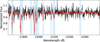 |
Fig. 5 Observed spectrum of NGC 6822-103 (in black) and best-fitting model (in red). The shaded blue regions highlight the spectral windows considered for the fitting process. The lines used for the fitting process from left to right by species are Fe I λλ 11 882.847, 11 973.050; Ti I λλ 11 892.878, 11 949.542; Si I λλ 11 984.20, 11 991.57, 12 031.50, 12 103.54, 12 270.50; Mg I λλ 11 828.185, 12083.346. |
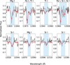 |
Fig. 6 Same as Fig. 5, but showing only the fitted spectral regions and the area around them. The contours represent the 68.3% confidence level errors. The spectral lines in each window are identified at the top of each panel. |
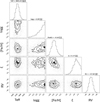 |
Fig. 7 Cornerplot showing the samples from the posterior distribution of Teff, log g, [Fe/H], ξ, and radial velocity prior to the heliocentric correction (RV) for NGC 6822-103. The solution vector is (Teff, log g, [Fe/H], ξ, RV=(3845.23 K, 0.29, −0.54, 5.17 km s−1,−57.50 km s−1). Unfortunately, log g is not well constrained. Contours represent regions of highest posterior probability, and their shape highlights potential correlations. |
Properties of the light curves.
4.2 Light curve results
The L-S periodogram analysis yielded significant periods for 3 sources, namely NGC 6822-52, IC10-26089, and WLM 14. The periodograms are presented in Appendix E. The periods are within the expected range for RSGs (i.e. 300–1000 days, see Chatys et al. 2019). In the case of IC10-26089, only the ZTF-r band was usable. The periodograms of the other objects either revealed nonperiodic behavior or the signal was too noisy; therefore, no periods can be reported. Next, we calculated the expected periods of our sources based on the Ks-band P–L relations of Yang & Jiang (2012, determined in the SMC) and Chatys et al. (2019, determined for Galactic RSGs), which have been found to be universal (Ren et al. 2019, i.e., their slopes are in agreement within uncertainties). The photometry was taken from Table 2 and the distances from Table 1. Table 5 contains all the properties determined using the light curves: the absolute Ks magnitudes (MKs), the periods measured using the L-S periodograms, the expected periods calculated using the Ks-band P–L relations, the luminosity, the amplitude in rZTF and W1 and the mass-loss rates. The luminosity is taken from de Wit et al. (2025), who measured it using SED fitting. The mass-loss rates for the NGC 6822 targets are taken from Antoniadis et al. (2025). We note that the absolute magnitude for IC10-26089 (MKs = −10.22 mag) is inconsistent with its high luminosity (log L/L⊙ = 5.25), and the P–L periods are shorter than expected. The 2MASS photometry was obtained in 1997–2001, a time period for which we have no light curve coverage; therefore, we have no knowledge of how the variability of the object could have affected the measurement. However, the SED fit from de Wit et al. (2025) is trustworthy.
We find two of our targets in NGC 6822 to display unusual variability (ΔrZTF > 1 mag, as variability of ~1 mag is typical for RSGs, Levesque 2017), namely NGC 6822-52 and NGC 6822-175 (see Table 5 and Fig. 4, Fig. D.5, respectively). Both the ΔrZTF of 2.5 mag and ΔW1 of 0.5 mag of NGC 6822-52 suggest an unusually strong pulsation. Such pulsations may occur during the last 104 yr of their lifetime (Heger et al. 1997). Currently, there are not enough available data to explore this possibility for NGC 6822-52. In the case of NGC 6822-175, its variability could be attributed to such a pulsation as well, despite its lower luminosity (de Wit et al. 2025).
We searched the light curves for dimming events. These outstanding events display variability greater than 1 magnitude and have a bell-like shape (see e.g., Fig. 4 of Munoz-Sanchez et al. 2024a). We found a candidate-dimming event in NGC 6822-175, with an estimated duration of 550 days (between MJD 58 292–58 762) and an amplitude exceeding 1.1 mag in the rZTF light curve. The exact amplitude and nature are uncertain because the minimum lacks photometric coverage. ZTF only covers the decrease in magnitude and the recovery. This event is also present in the WISE W1 light curve, with an amplitude of ~0.5 mag, as there is a local minimum during the time span of the event. Fig. 8 compares the candidate-dimming event in rZTF to the AAVSO photometry of the Great Dimming of Betelgeuse and overplots the W1 light curve. We discuss the properties of this candidate-dimming event in Sect. 5.4. We note that the semiperiodic variability in the optical light curve in the ~1000 days preceding the event displayed minima with increasing depth, while after the dimming, the minima became shallower. The same behavior is observed in the infrared light curve (Fig. D.5).
4.3 Evidence for episodic mass loss
Episodic mass loss can be traced by taking into account both the photometric and spectroscopic variability of our sources. Specifically, we search for nontypical photometric and spectral variability. Also, we calculate the median absolute deviation in W1 (MADW1) and compare it to the right panel of Fig. 12 of Yang et al. (2023). If the object lies in the region after the “kink” feature where mass-loss rates increase, it is an indication of strong mid-IR variability, meaning that either it has experienced or will experience episodic mass loss. Thus, we identify four targets out of seven that exhibit evidence for episodic mass loss:
NGC 6822-52 has a high luminosity (log(LSED/L⊙)= 5.10) and a long period (693 days). It is the most photometrically variable star (ΔrZTF ~ 2.5 mag and ΔW1 ~ 0.5 mag) in the sample (Fig. 4). It also displays spectroscopic variability transitioning from a spectral type of M1 to M4 within ~40 years (see Table 2). It has a MADW1 value of 0.10 mag and, given its luminosity, it is situated after the kink feature. Considering all the information presented above and its IR excess, we conclude that it is a strong candidate for episodic mass loss.
NGC 6822-55 is one of the most luminous (log(LSED/L⊙) = 5.21) sources in our sample. Its light curve displays significant variability (ΔrZTF ~ 0.8 mag and ΔW1 ~ 0.3 mag; Fig. D.2). Its spectral type has changed from M0 to K7 between 2008 and 2020 (see Table 2), indicating that we have a K-type RSG with IR excess. The mid-IR photometry was obtained at a different epoch, indicating that the object was in a cooler, more extended state and therefore losing mass at a higher rate. This caused its colors to be redder due to the formation of dust. It has since returned to a hotter, more compact state observed by spectroscopy (de Wit et al. 2024). Furthermore, de Wit et al. (2025) report that given its low mass-loss rate (see Table 5), an eruptive mass-loss event should have taken place to produce the increased amounts of dust measured by the mid-IR photometry. Its MADW1 value is 0.05 mag; therefore, it is located clearly after the kink feature, favoring the episodic mass loss scenario. The J-band Teff derived in this work is higher than the one estimated by Patrick et al. (2015, spectrum obtained in 2013), confirming this temperature rise.
IC10-26089 is the most luminous source in our sample (log(LSED/L⊙) = 5.25), yet it has a small period (482 days). It has a K4 spectral type; however, its position in the CMD (Fig. 1) suggests that it is a dusty star. This behavior is similar to NGC 6822-55, indicating that we have identified another candidate for episodic mass loss. Once again, its MADW1 value of 0.06 mag means that it can be found after the kink feature, favoring the scenario of a past eruptive mass-loss event. However, we do not have a mass-loss rate estimation, and there is no other optical spectrum in the literature for this target. Also, we were unable to model its J-band spectrum. It displays strong photometric variability (ΔrZTF ~ 0.9 mag and ΔW1 ~ 0.5 mag; Fig. D.1).
NGC 6822-175 has the lowest luminosity (log(LSED/L⊙) = 4.80) of the sample and the smallest period (376 days). It has a candidate-dimming event in its light curve (ΔrZTF > 1.1 mag and ΔW1 ~ 0.5 mag; Fig. D.5), a typical indication of episodic mass loss. Its mass-loss rate is similar to NGC 6822-70. It also experiences spectral variability, transitioning from M1 to M4 between 2008 and 2020. Along with its luminosity, its MADW1 value of 0.09 mag places it after the kink feature. Therefore, the star displays strong evidence of at least one significant past mass ejection.
NGC 6822-70 exhibits moderate photometric variability (ΔrZTF ~ 0.7 mag and ΔW1 ~ 0.3 mag; Fig. D.3); however, there is no other optical spectrum in the literature. Similarly, NGC 6822-103, the target with the highest mass-loss rate (see Table 5), displays mild photometric variability (ΔrZTF ~ 0.6 mag and ΔW1 ~ 0.2 mag; Fig. D.4) as well but there is no other evidence for episodic mass loss. Also, the position of WLM 14 in the CMD does not suggest a dusty star. It displays no spectral variability; however, its photometric variability is also modest (ΔrZTF ~ 0.7 mag and ΔW1 ~ 0.3 mag; Fig. D.6). Currently, there is no mass-loss rate estimation for this target. However, this could be potentially revisited in the future using James Webb Space Telescope (JWST) data now available for WLM.
To determine whether moderate photometric variability is a sufficient clue for episodic mass loss, we calculated the MADW1 for NGC 6822-103, NGC 6822-70 and WLM 14 and found values of 0.05, 0.04 and 0.06 mag, respectively, meaning that the objects lie in the region after the kink feature therefore they could experience episodic mass loss in the future or, if they have already experienced such events, that we just do not have the data to trace them.
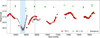 |
Fig. 8 Zoom-in on the candidate-dimming event (marked with the dashed dotted lines) in the rZTF and W1-band light curves of NGC 6822-175. Possible locations of the minimum are highlighted with the shaded region. The dimming event of Betelgeuse is shown for comparison (gray triangles). Data were retrieved from the AAVSO database. |
5 Discussion
5.1 Hertzsprung–Russell diagram
We present a Hertzsprung–Russell (HR) diagram, where we compare our sample to evolutionary tracks and search for outliers (Fig. 9). We include mist stellar tracks (Dotter 2016; Choi et al. 2016) for rotating stars (v/vcrit = 0.4) of 10, 15, 20 and 25 M⊙ and [Fe/H]=−0.50 to compare the evolutionary predictions to the evolutionary status of our targets, given by their derived Teff and log L. We choose the MIST tracks over the Geneva ones because the former provide a better match to the high-mass RSG population of the LMC (Yang et al. 2021; de Wit et al. 2023). As most of our targets reside in NGC 6822, we use tracks consistent with its average metallicity value of [Z]=–0.52 reported by Patrick et al. (2015). We assume that [Z]=[Fe/H], following the assumptions made in the same work. For each source, we show both the ![Mathematical equation: $\[T_{\text {eff}}^{\mathrm{TiO}}\]$](/articles/aa/full_html/2025/12/aa54071-25/aa54071-25-eq53.png) (empty stars) from de Wit et al. (2025) and
(empty stars) from de Wit et al. (2025) and ![Mathematical equation: $\[T_{\text {eff}}^{J, \text {fit}}\]$](/articles/aa/full_html/2025/12/aa54071-25/aa54071-25-eq54.png) (red stars) calculated in this work. For NGC 6822-52 and IC10-26089 we only present the
(red stars) calculated in this work. For NGC 6822-52 and IC10-26089 we only present the ![Mathematical equation: $\[T_{\text {eff}}^{\mathrm{TiO}}\]$](/articles/aa/full_html/2025/12/aa54071-25/aa54071-25-eq55.png) .
.
We limit our HR diagram to the region occupied by RSGs. Specifically, Antoniadis et al. (2025) have determined a luminosity range between 3.2 and 5.26 for their candidate RSGs in NGC 6822. However, it is unclear whether objects with log(L/L⊙) < 4 are in fact RSGs or asymptotic giant branch stars (see e.g., Yang et al. 2024). Therefore, we adopt the widely accepted lower limit of log(L/L⊙) = 4 for RSGs. Furthermore, there is some controversy about the upper luminosity limit of RSGs (Humphreys & Davidson 1979; Davies et al. 2018; McDonald et al. 2022; Munoz-Sanchez et al. 2024b; Maravelias et al. 2025). We adopted an upper limit of log(L/L⊙) = 5.5.
We note that NGC 6822-70 and NGC 6822-175 are close to the Hayashi limit when considering their ![Mathematical equation: $\[T_{\text {eff}}^{\mathrm{TiO}}\]$](/articles/aa/full_html/2025/12/aa54071-25/aa54071-25-eq58.png) . However, when we take into account their
. However, when we take into account their ![Mathematical equation: $\[T_{\text {eff}}^{J, \text {fit}}\]$](/articles/aa/full_html/2025/12/aa54071-25/aa54071-25-eq59.png) , they are brought back to the permitted region of the HR diagram. We attribute this behavior to the fact that the TiO-band method provides cooler Teff estimates. We remark that in the case of NGC 6822-175 the discrepancy between the
, they are brought back to the permitted region of the HR diagram. We attribute this behavior to the fact that the TiO-band method provides cooler Teff estimates. We remark that in the case of NGC 6822-175 the discrepancy between the ![Mathematical equation: $\[T_{\text {eff}}^{J, \text {fit}}\]$](/articles/aa/full_html/2025/12/aa54071-25/aa54071-25-eq60.png) and the
and the ![Mathematical equation: $\[T_{\text {eff}}^{\mathrm{TiO}}\]$](/articles/aa/full_html/2025/12/aa54071-25/aa54071-25-eq61.png) cannot be explained by the shortcomings of the TiO-band method alone (which are responsible for differences of 100–200 K, see Davies et al. 2013). We do not find any of our targets to be outliers in the HR diagram, especially when their J-band temperatures are taken into account.
cannot be explained by the shortcomings of the TiO-band method alone (which are responsible for differences of 100–200 K, see Davies et al. 2013). We do not find any of our targets to be outliers in the HR diagram, especially when their J-band temperatures are taken into account.
We compare with the HR diagram constructed by Patrick et al. (2015, their Fig. 11) and find that most of our RSGs occupy the same luminosity regime (log L ≥ 4.8) but most of them are not in the same Teff regime, as theirs are at Teff ≤ 4000 K. Since we only have two targets in common with them and we achieved agreement within 3σ with their derived Teff (see previous sections) and our error bars are significantly larger than theirs (see Table 4), we refrain from drawing strong conclusions.
However, there are pitfalls to the evolutionary tracks. Specifically, MIST stellar tracks use a fixed value of 1.25 for the mixing length (αMT, Choi et al. 2016); however, recent studies have shown that fixing the αMT value is not optimal for all kinds of stars (e.g., Bonaca et al. 2012; Tayar et al. 2017). Furthermore, it is known that the mixing length has a metallicity dependence both for high and for low mass stars (Chun et al. 2018; Joyce & Chaboyer 2018), namely, it increases with metallicity (e.g., Bonaca et al. 2012). Furthermore, the MIST stellar tracks are calculated using 1D stellar atmosphere models; thus, they cannot describe 3D phenomena such as mass loss or convection (Choi et al. 2016), in turn failing to accurately predict the evolution of targets such as NGC 6822-55 and NGC 6822-175 (see previous sections).
We observe that ![Mathematical equation: $\[T_{\text {eff}}^{J, \text {fit}}\]$](/articles/aa/full_html/2025/12/aa54071-25/aa54071-25-eq62.png) are not near the Hayashi limit, as opposed to the
are not near the Hayashi limit, as opposed to the ![Mathematical equation: $\[T_{\text {eff}}^{\mathrm{TiO}}\]$](/articles/aa/full_html/2025/12/aa54071-25/aa54071-25-eq63.png) . This is a known limitation of the
. This is a known limitation of the ![Mathematical equation: $\[T_{\text {eff}}^{J, \text {fit}}\]$](/articles/aa/full_html/2025/12/aa54071-25/aa54071-25-eq64.png) values (see Fig. 9 of Patrick et al. 2015) that applies to the
values (see Fig. 9 of Patrick et al. 2015) that applies to the ![Mathematical equation: $\[T_{\text {eff}, \mathrm{J}}^{scaled}\]$](/articles/aa/full_html/2025/12/aa54071-25/aa54071-25-eq65.png) as well (de Wit et al. 2024, see the left panel of their Fig. 14). However, the Hayashi limit shifts to higher temperatures for lower metallicities and higher mixing length values. Chun et al. (2022) has shown that for low metallicity, a mixing length value of ~2–2.5 shifts the Hayashi limit to the
as well (de Wit et al. 2024, see the left panel of their Fig. 14). However, the Hayashi limit shifts to higher temperatures for lower metallicities and higher mixing length values. Chun et al. (2022) has shown that for low metallicity, a mixing length value of ~2–2.5 shifts the Hayashi limit to the ![Mathematical equation: $\[T_{\text {eff}}^{J, \text {fit}}\]$](/articles/aa/full_html/2025/12/aa54071-25/aa54071-25-eq66.png) locus (see their Figs. 5 and 6). Therefore, we speculate that stellar tracks with a αMT value within this range could place the Hayashi limit closer to our
locus (see their Figs. 5 and 6). Therefore, we speculate that stellar tracks with a αMT value within this range could place the Hayashi limit closer to our ![Mathematical equation: $\[T_{\text {eff}}^{J, \text {fit}}\]$](/articles/aa/full_html/2025/12/aa54071-25/aa54071-25-eq67.png) values.
values.
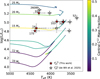 |
Fig. 9 HR diagram for targets with luminosity estimates. Red stars denote the |
![Mathematical equation: $\[T_{\text {eff}}^{J, \text {fit}}\]$](/articles/aa/full_html/2025/12/aa54071-25/aa54071-25-eq56.png)
![Mathematical equation: $\[T_{\text {eff}}^{\mathrm{TiO}}\]$](/articles/aa/full_html/2025/12/aa54071-25/aa54071-25-eq57.png)
5.2 Effective temperatures
We compare the effective temperatures obtained for our targets using the various methods described above, searching for overall trends. The ![Mathematical equation: $\[T_{\text {eff}}^{\mathrm{TiO}}\]$](/articles/aa/full_html/2025/12/aa54071-25/aa54071-25-eq68.png) temperatures obtained from modeling the TiO bands are lower than the
temperatures obtained from modeling the TiO bands are lower than the ![Mathematical equation: $\[T_{\text {eff}}^{J, \text {fit}}\]$](/articles/aa/full_html/2025/12/aa54071-25/aa54071-25-eq69.png) obtained by fitting the J-band. This is in agreement with the conclusions of Davies et al. (2013) and is also valid for our derived
obtained by fitting the J-band. This is in agreement with the conclusions of Davies et al. (2013) and is also valid for our derived ![Mathematical equation: $\[T_{\text {eff}, \mathrm{J}}^{scaled}\]$](/articles/aa/full_html/2025/12/aa54071-25/aa54071-25-eq70.png) . We note that for the four targets we have in common with Dimitrova et al. (2022), namely NGC 6822-52, NGC 6822-70, NGC 6822-103 and NGC 6822-175, the Teff values determined in that work (
. We note that for the four targets we have in common with Dimitrova et al. (2022), namely NGC 6822-52, NGC 6822-70, NGC 6822-103 and NGC 6822-175, the Teff values determined in that work (![Mathematical equation: $\[T_{\text {eff }}^{J-K}\]$](/articles/aa/full_html/2025/12/aa54071-25/aa54071-25-eq71.png) ) are only hotter than
) are only hotter than ![Mathematical equation: $\[T_{\text {eff}}^{\mathrm{TiO}}\]$](/articles/aa/full_html/2025/12/aa54071-25/aa54071-25-eq72.png) . In contrast, in the case of IC10-26089, which was also studied by Dimitrova et al. (2020), their
. In contrast, in the case of IC10-26089, which was also studied by Dimitrova et al. (2020), their ![Mathematical equation: $\[T_{\text {eff }}^{J-K}\]$](/articles/aa/full_html/2025/12/aa54071-25/aa54071-25-eq73.png) value is the lowest one measured for the object. Furthermore,
value is the lowest one measured for the object. Furthermore, ![Mathematical equation: $\[T_{\text {eff}}^{J-K_{s}}\]$](/articles/aa/full_html/2025/12/aa54071-25/aa54071-25-eq74.png) and
and ![Mathematical equation: $\[T_{\text {eff}}^{\text {MARCS}}\]$](/articles/aa/full_html/2025/12/aa54071-25/aa54071-25-eq75.png) are in agreement within the error bars for all of our objects. For most of our targets, both
are in agreement within the error bars for all of our objects. For most of our targets, both ![Mathematical equation: $\[T_{\text {eff}}^{J, \text {fit}}\]$](/articles/aa/full_html/2025/12/aa54071-25/aa54071-25-eq76.png) and
and ![Mathematical equation: $\[T_{\text {eff}, \mathrm{J}}^{scaled}\]$](/articles/aa/full_html/2025/12/aa54071-25/aa54071-25-eq77.png) are even hotter than
are even hotter than ![Mathematical equation: $\[T_{\text {eff}}^{J-K_{s}}\]$](/articles/aa/full_html/2025/12/aa54071-25/aa54071-25-eq78.png) . Notable exceptions are NGC 6822-103 and NGC 6822-70 where
. Notable exceptions are NGC 6822-103 and NGC 6822-70 where ![Mathematical equation: $\[T_{\text {eff}}^{J-K_{s}}\]$](/articles/aa/full_html/2025/12/aa54071-25/aa54071-25-eq79.png) values are hotter than
values are hotter than ![Mathematical equation: $\[T_{\text {eff}}^{J, \text {fit}}\]$](/articles/aa/full_html/2025/12/aa54071-25/aa54071-25-eq80.png) but cooler than
but cooler than ![Mathematical equation: $\[T_{\text {eff}, \mathrm{J}}^{scaled}\]$](/articles/aa/full_html/2025/12/aa54071-25/aa54071-25-eq81.png) . In the case of NGC 6822-55
. In the case of NGC 6822-55 ![Mathematical equation: $\[T_{\text {eff}}^{J-K_{s}}\]$](/articles/aa/full_html/2025/12/aa54071-25/aa54071-25-eq82.png) ,
, ![Mathematical equation: $\[T_{\text {eff}}^{\text {MARCS}}\]$](/articles/aa/full_html/2025/12/aa54071-25/aa54071-25-eq83.png) ,
, ![Mathematical equation: $\[T_{\text {eff}}^{\mathrm{TiO}}\]$](/articles/aa/full_html/2025/12/aa54071-25/aa54071-25-eq84.png) and
and ![Mathematical equation: $\[T_{\text {eff}, \mathrm{J}}^{scaled}\]$](/articles/aa/full_html/2025/12/aa54071-25/aa54071-25-eq85.png) agree within the error bars, whereas for NGC 6822-175
agree within the error bars, whereas for NGC 6822-175 ![Mathematical equation: $\[T_{\text {eff }}^{J, \mathrm{P} 15}\]$](/articles/aa/full_html/2025/12/aa54071-25/aa54071-25-eq86.png) ,
, ![Mathematical equation: $\[T_{\text {eff}}^{J-K_{s}}\]$](/articles/aa/full_html/2025/12/aa54071-25/aa54071-25-eq87.png) and
and ![Mathematical equation: $\[T_{\text {eff}}^{\text {MARCS}}\]$](/articles/aa/full_html/2025/12/aa54071-25/aa54071-25-eq88.png) are in agreement within the error bars. Finally, we highlight that in the respective cases of NGC 6822-103 and NGC 6822-175, the values of our error bars are comparable with the ones obtained by Patrick et al. (2015).
are in agreement within the error bars. Finally, we highlight that in the respective cases of NGC 6822-103 and NGC 6822-175, the values of our error bars are comparable with the ones obtained by Patrick et al. (2015).
We note the case of WLM 14 where the effective temperatures obtained have a ~500 K span. The relation used to calculate ![Mathematical equation: $\[T_{\text {eff}}^{J-K_{s}}\]$](/articles/aa/full_html/2025/12/aa54071-25/aa54071-25-eq89.png) (see Table 4) was calibrated on a sample of RSGs located in the Magellanic Clouds where the metallicity ranges from 0.2 to 0.79 Z⊙ (see Table 5 of de Wit et al. 2024, for details), whereas the metallicity of WLM is lower (see Table 1); therefore, we extrapolated the relation to obtain this value. We are unable to use the scaling relation for NGC 6822-52 because its
(see Table 4) was calibrated on a sample of RSGs located in the Magellanic Clouds where the metallicity ranges from 0.2 to 0.79 Z⊙ (see Table 5 of de Wit et al. 2024, for details), whereas the metallicity of WLM is lower (see Table 1); therefore, we extrapolated the relation to obtain this value. We are unable to use the scaling relation for NGC 6822-52 because its ![Mathematical equation: $\[T_{\text {eff}}^{\mathrm{TiO}}\]$](/articles/aa/full_html/2025/12/aa54071-25/aa54071-25-eq90.png) value is below the Teff range where the relation is applicable (see Sect. 4.3 of de Wit et al. 2024). Furthermore, this
value is below the Teff range where the relation is applicable (see Sect. 4.3 of de Wit et al. 2024). Furthermore, this ![Mathematical equation: $\[T_{\text {eff}}^{\mathrm{TiO}}\]$](/articles/aa/full_html/2025/12/aa54071-25/aa54071-25-eq91.png) value is close to the lower edge of the grid of de Wit et al. (2025), so we urge caution in its interpretation. As a final note, when we cross-matched our IC 10 target with the catalog of Dimitrova et al. (2020), we found two sources with identical coordinates matching within a 1.0″ radius. We selected the target with a Gaia parallax to be the correct match, as our target had a Gaia parallax.
value is close to the lower edge of the grid of de Wit et al. (2025), so we urge caution in its interpretation. As a final note, when we cross-matched our IC 10 target with the catalog of Dimitrova et al. (2020), we found two sources with identical coordinates matching within a 1.0″ radius. We selected the target with a Gaia parallax to be the correct match, as our target had a Gaia parallax.
5.3 Metallicity
Patrick et al. (2015) report that NGC 6822 has a low significance metallicity gradient within 1 kpc from the galactic center utilizing 11 RSGs. Specifically, as the distance from the galactic center increases, the metallicity decreases. They report an average metallicity of −0.52, while individual RSGs have values ranging from −0.20 to −0.78. This average value is consistent with the values reported by studies that utilized blue supergiants (Muschielok et al. 1999; Venn et al. 2001).
We have modeled 4 targets in NGC 6822. For NGC 6822-55, which is at the center of the galaxy, we find a metallicity value of −0.50. For NGC 6822-70 and NGC 6822-175, which are located in the outer part of the galaxy, we find −0.83 and −0.81, respectively. Given the objects’ respective locations, these values are anticipated. However, NGC 6822-103 has a metallicity value of −0.54, although it is situated on the outskirts of the galaxy.
5.4 Candidate-dimming event
We compare the properties of the proposed dimming event in NGC 6822-175 to events that have occurred in other RSGs, and in particular Betelgeuse. We argue that the light curve of NGC 6822-175 after the candidate-dimming event could be similar to that of Betelgeuse after its own dimming episode known as the “Great Dimming” (Montargès et al. 2021; Dupree et al. 2022), see Jadlovský et al. (2024) for a recent light curve, but because of the limited coverage compared to Betelgeuse, we refrain from drawing strong conclusions. Studies of Betelgeuse after the Great Dimming have shown that it exhibits smaller amplitude variability, pulsating in its first overtone, which has a period of ~200 d (i.e., half of its period before the Great Dimming; Granzer et al. 2022). Betelgeuse is predicted to revert to its pre-Great Dimming behavior within the next 5–10 yr (MacLeod et al. 2023). It is likely that our source could exhibit similar behavior. In the case of [W60] B90, dimming events are recurring (with a periodicity of ~11.8 yr, see Munoz-Sanchez et al. 2024a); however, for other RSGs such as Betelgeuse and RW Cep, the dimming events are unique on a timescale of 100 yr. As we do not have a period for NGC 6822-175 (see Table 5), we cannot compare directly with Betelgeuse or [W60] B90. NGC 6822-175 (log L/L⊙ = 4.8, see Table 5) is less luminous than Betelgeuse and [W60] B90 (log L/L⊙ = 5.10 and 5.32, respectively; see Table 5 of Munoz-Sanchez et al. 2024a). Our light curve coverage stops ~5.5 yr after the event, in which no other dimming event has been detected. This interval is likely too short for us to draw any meaningful conclusions or make reliable predictions regarding the source’s behavior.
Recently, Munoz-Sanchez et al. (2024a) suggested that the timescale of these events is connected to the radius of the RSGs that host them, as more extended atmospheres need more time to return to stability. Using the Stefan-Boltzmann law, we estimated the radius of NGC 6822-175 to be within the range of 530–678 R⊙ depending on Teff (see Table 4), which is close to the lower end of the radii range reported for Betelgeuse (750–1000 R⊙, Joyce et al. 2020; Kravchenko et al. 2021). The rise time for NGC 6822-175 after its event is ~200–300 days, depending on the possible locations of the minimum (see Fig. 8), which is similar to Betelgeuse, but only around half the recovery time of [W60] B90, which has a significantly larger radius (~1200 R⊙, Munoz-Sanchez et al. 2024a). This result further supports the proposed connection between the radius of RSGs and the timescale of their dimming events.
6 Summary and conclusions
We have conducted a comprehensive study of seven mass-losing RSGs in nearby low-metallicity galaxies. We obtained usable spectra for five out of seven targets with EMIR on GTC. We modeled these spectra using MARCS models corrected for nonlocal thermal equilibrium effects and obtained physical parameters for these RSGs. Additionally, we calculated Teff values for all of our targets using empirical and scaling relations presented in de Wit et al. (2024), which are in agreement with the values determined by the modeling. We presented their optical, near-IR, and mid-IR light curves, discovering two RSGs (NGC 6822-52 and NGC 6822-175) with unusual photometric variability. The light curves yielded periods for three RSGs. We discovered a candidate-dimming event in NGC 6822-175 with an estimated duration of 550 days and depth in r over 1.1 mag. Monitoring of this object could reveal whether this phenomenon is recurring or if this was a unique event. We also improved the spectral classification from the available optical spectra, finding four sources exhibiting spectral variability.
Combining all of our results, we identified four RSGs (NGC 6822-52, NGC 6822-55, NGC 6822-175, and IC10-26089) that are candidates for having undergone episodic mass loss. We suggest that NGC 6822-70, NGC 6822-103, and WLM 14 can be confirmed as candidates for episodic mass loss with additional spectroscopy. This work shows that both multi-epoch spectroscopy and time-series photometry are valuable for the characterization of episodic mass loss for dusty RSGs, as they trace the changes it causes to the stellar atmospheres.
However, RSGs with episodic mass loss are rare (de Wit et al. 2024). The development of machine–learning photometric classifiers (e.g., Maravelias et al. 2022) enables studies of large samples of RSGs (over 100 000 RSGc in ~20 nearby galaxies have been identified by Maravelias et al. (2025)) and the characterization of the frequency of episodic mass loss, shedding light on their mass-loss history. Future surveys such as the Rubin Observatory Legacy Survey of Space and Time (LSST) will provide light curves for many objects, and JWST is providing mid-IR photometry, critical for collecting large samples of targets in distant galaxies. Along with spectroscopy, these data will be paramount to discovering RSGs with episodic mass loss and Levesque–Massey variables, as well as determining the physical mechanisms causing these phenomena.
Acknowledgements
E.C., S.d.W., A.Z.B., G.M.S., G.M., and K.A. acknowledge funding support from the European Research Council (ERC) under the European Union’s Horizon 2020 research and innovation program (“ASSESS”, Grant agreement No. 772086). M.M.R-D acknowledges financial support through Spanish grant PID2019-105552RB-C41(MCIU) and from Comunidad de Madrid through the Estimulo a la Excelencia para Profesores Universitarios Permanentes (EPDU-INV/2020/008). Based on observations made with the Gran Telescopio Canarias (GTC), installed at the Spanish Observatorio del Roque de los Muchachos of the Instituto de Astrofísica de Canarias, on the island of La Palma. This work is (partly) based on data obtained with the instrument EMIR, built by a Consortium led by the Instituto de Astrofísica de Canarias. EMIR was funded by GRANTECAN and the National Plan of Astronomy and Astrophysics of the Spanish Government. This work is based in part on observations made with the Spitzer Space Telescope, which is operated by the Jet Propulsion Laboratory, California Institute of Technology, under a contract with NASA. This work has made use of data from the European Space Agency (ESA) mission Gaia (https://www.cosmos.esa.int/gaia), processed by the Gaia Data Processing and Analysis Consortium (DPAC, https://www.cosmos.esa.int/web/gaia/dpac/consortium). Funding for the DPAC has been provided by national institutions, in particular the institutions participating in the Gaia Multilateral Agreement. We acknowledge with thanks the variable star observations from the AAVSO International Database contributed by observers worldwide and used in this research. We thank John Pritchard for his valuable assistance with the Molecfit installation and execution. We thank Lee Patrick for providing his catalog of RSG candidates and for useful discussions during various stages of the paper. We thank Patricia Whitelock and John Menzies for providing us with their J H Ks photometric data. We thank Despina Hatzidimitriou, Philip Wiseman, and Karan Dsilva for useful discussions.
References
- Antoniadis, K., Bonanos, A. Z., de Wit, S., et al. 2024, A&A, 686, A88 [NASA ADS] [CrossRef] [EDP Sciences] [Google Scholar]
- Antoniadis, K., Zapartas, E., Bonanos, A. Z., et al. 2025, A&A, 702, A178 [NASA ADS] [CrossRef] [EDP Sciences] [Google Scholar]
- Anugu, N., Baron, F., Gies, D. R., et al. 2023, AJ, 166, 78 [NASA ADS] [CrossRef] [Google Scholar]
- Asplund, M., Grevesse, N., Sauval, A. J., & Scott, P. 2009, ARA&A, 47, 481 [NASA ADS] [CrossRef] [Google Scholar]
- Beasor, E. R., Davies, B., Smith, N., et al. 2020, MNRAS, 492, 5994 [Google Scholar]
- Bellm, E. C., Kulkarni, S. R., Graham, M. J., et al. 2019, PASP, 131, 018002 [Google Scholar]
- Bergemann, M., Lind, K., Collet, R., et al. 2012, MNRAS, 427, 27 [NASA ADS] [CrossRef] [Google Scholar]
- Bergemann, M., Kudritzki, R.-P., Würl, M., et al. 2013, ApJ, 764, 115 [NASA ADS] [CrossRef] [Google Scholar]
- Bergemann, M., Kudritzki, R.-P., Gazak, Z., et al. 2015, ApJ, 804, 113 [NASA ADS] [CrossRef] [Google Scholar]
- Bonaca, A., Tanner, J. D., Basu, S., et al. 2012, ApJ, 755, L12 [NASA ADS] [CrossRef] [Google Scholar]
- Bonanos, A. Z., Tramper, F., de Wit, S., et al. 2024, A&A, 686, A77 [NASA ADS] [CrossRef] [EDP Sciences] [Google Scholar]
- Bresolin, F., Pietrzyński, G., Urbaneja, M. A., et al. 2006, ApJ, 648, 1007 [NASA ADS] [CrossRef] [Google Scholar]
- Britavskiy, N. E., Bonanos, A. Z., Mehner, A., Boyer, M. L., & McQuinn, K. B. W. 2015, A&A, 584, A33 [NASA ADS] [CrossRef] [EDP Sciences] [Google Scholar]
- Britavskiy, N. E., Bonanos, A. Z., Herrero, A., et al. 2019, A&A, 631, A95 [NASA ADS] [CrossRef] [EDP Sciences] [Google Scholar]
- Buchner, J. 2021, J. Open Source Softw., 6, 3001 [CrossRef] [Google Scholar]
- Chambers, K. C., Magnier, E. A., Metcalfe, N., et al. 2016, arXiv e-prints [arXiv:1612.05560] [Google Scholar]
- Chatys, F. W., Bedding, T. R., Murphy, S. J., et al. 2019, MNRAS, 487, 4832 [CrossRef] [Google Scholar]
- Chiavassa, A., Plez, B., Josselin, E., & Freytag, B. 2009, A&A, 506, 1351 [NASA ADS] [CrossRef] [EDP Sciences] [Google Scholar]
- Choi, J., Dotter, A., Conroy, C., et al. 2016, ApJ, 823, 102 [Google Scholar]
- Chun, S.-H., Yoon, S.-C., Jung, M.-K., Kim, D. U., & Kim, J. 2018, ApJ, 853, 79 [NASA ADS] [CrossRef] [Google Scholar]
- Chun, S.-H., Yoon, S.-C., Oh, H., Park, B.-G., & Hwang, N. 2022, ApJ, 939, 28 [NASA ADS] [CrossRef] [Google Scholar]
- Davies, B., & Plez, B. 2021, MNRAS, 508, 5757 [NASA ADS] [CrossRef] [Google Scholar]
- Davies, B., Kudritzki, R.-P., & Figer, D. F. 2010, MNRAS, 407, 1203 [NASA ADS] [CrossRef] [Google Scholar]
- Davies, B., Kudritzki, R.-P., Plez, B., et al. 2013, ApJ, 767, 3 [Google Scholar]
- Davies, B., Kudritzki, R.-P., Gazak, Z., et al. 2015, ApJ, 806, 21 [NASA ADS] [CrossRef] [Google Scholar]
- Davies, B., Crowther, P. A., & Beasor, E. R. 2018, MNRAS, 478, 3138 [NASA ADS] [CrossRef] [Google Scholar]
- de Wit, S., Bonanos, A. Z., Tramper, F., et al. 2023, A&A, 669, A86 [NASA ADS] [CrossRef] [EDP Sciences] [Google Scholar]
- de Wit, S., Bonanos, A. Z., Antoniadis, K., et al. 2024, A&A, 689, A46 [NASA ADS] [CrossRef] [EDP Sciences] [Google Scholar]
- de Wit, S., Muñoz-Sanchez, G., Maravelias, G., et al. 2025, A&A, 698, A279 [NASA ADS] [CrossRef] [EDP Sciences] [Google Scholar]
- Decin, L. 2021, ARA&A, 59, 337 [NASA ADS] [CrossRef] [Google Scholar]
- Dimitrova, T. A., Neugent, K. F., Levesque, E. M., & Massey, P. 2020, Res. Notes Am. Astron. Soc., 4, 107 [Google Scholar]
- Dimitrova, T. A., Neugent, K. F., Massey, P., & Levesque, E. M. 2022, AJ, 163, 70 [Google Scholar]
- Dopita, M. A., Seitenzahl, I. R., Sutherland, R. S., et al. 2019, AJ, 157, 50 [Google Scholar]
- Dorda, R., & Patrick, L. R. 2021, MNRAS, 502, 4890 [NASA ADS] [CrossRef] [Google Scholar]
- Dorda, R., Negueruela, I., González-Fernández, C., & Tabernero, H. M. 2016, A&A, 592, A16 [NASA ADS] [CrossRef] [EDP Sciences] [Google Scholar]
- Dotter, A. 2016, ApJS, 222, 8 [Google Scholar]
- Dupree, A. K., Strassmeier, K. G., Calderwood, T., et al. 2022, ApJ, 936, 18 [NASA ADS] [CrossRef] [Google Scholar]
- Evans, C. J., Davies, B., Kudritzki, R. P., et al. 2011, A&A, 527, A50 [NASA ADS] [CrossRef] [EDP Sciences] [Google Scholar]
- Freytag, B., Steffen, M., & Dorch, B. 2002, Astron. Nachri., 323, 213 [NASA ADS] [CrossRef] [Google Scholar]
- Freytag, B., Steffen, M., Ludwig, H. G., et al. 2012, J. Comput. Phys., 231, 919 [Google Scholar]
- Freytag, B., Höfner, S., Aringer, B., & Chiavassa, A. 2024, A&A, 692, A223 [NASA ADS] [CrossRef] [EDP Sciences] [Google Scholar]
- Gaia Collaboration (Prusti, T., et al.) 2016, A&A, 595, A1 [NASA ADS] [CrossRef] [EDP Sciences] [Google Scholar]
- Gaia Collaboration (Vallenari, A., et al.) 2023, A&A, 674, A1 [NASA ADS] [CrossRef] [EDP Sciences] [Google Scholar]
- Garzón, F., Balcells, M., Gallego, J., et al. 2022, A&A, 667, A107 [CrossRef] [EDP Sciences] [Google Scholar]
- Garzón, F., Fernández-Acosta, S., Hammersley, P., et al. 2024, SPIE, 13096, 1309627 [Google Scholar]
- Gazak, J. Z., Davies, B., Kudritzki, R., Bergemann, M., & Plez, B. 2014, ApJ, 788, 58 [NASA ADS] [CrossRef] [Google Scholar]
- Georgy, C. 2012, A&A, 538, L8 [NASA ADS] [CrossRef] [EDP Sciences] [Google Scholar]
- Goldberg, J. A., Jiang, Y.-F., & Bildsten, L. 2022, ApJ, 929, 156 [NASA ADS] [CrossRef] [Google Scholar]
- Graham, M. J., Kulkarni, S. R., Bellm, E. C., et al. 2019, PASP, 131, 078001 [Google Scholar]
- Granzer, T., Weber, M., Strassmeier, K. G., & Dupree, A. 2022, in The 21st Cambridge Workshop on Cool Stars, Stellar Systems, and the Sun, Cambridge Workshop on Cool Stars, Stellar Systems, and the Sun, 185 [Google Scholar]
- Guinan, E. F., Wasatonic, R. J., & Calderwood, T. J. 2019, ATel, 13341, 1 [NASA ADS] [Google Scholar]
- Gustafsson, B., Edvardsson, B., Eriksson, K., et al. 2008, A&A, 486, 951 [NASA ADS] [CrossRef] [EDP Sciences] [Google Scholar]
- Heger, A., Jeannin, L., Langer, N., & Baraffe, I. 1997, A&A, 327, 224 [NASA ADS] [Google Scholar]
- Heger, A., Fryer, C. L., Woosley, S. E., et al. 2003, ApJ, 591, 288 [CrossRef] [Google Scholar]
- Heinze, A. N., Tonry, J. L., Denneau, L., et al. 2018, AJ, 156, 241 [Google Scholar]
- Humphreys, R. M. 1980, ApJ, 238, 65 [Google Scholar]
- Humphreys, R. M., & Davidson, K. 1979, ApJ, 232, 409 [Google Scholar]
- Humphreys, R. M., & Jones, T. J. 2022, AJ, 163, 103 [NASA ADS] [CrossRef] [Google Scholar]
- Hwang, H.-C., & Zakamska, N. L. 2020, MNRAS, 493, 2271 [NASA ADS] [CrossRef] [Google Scholar]
- Jadlovský, D., Granzer, T., Weber, M., et al. 2024, A&A, 685, A124 [NASA ADS] [CrossRef] [EDP Sciences] [Google Scholar]
- Josselin, E., & Plez, B. 2007, A&A, 469, 671 [NASA ADS] [CrossRef] [EDP Sciences] [Google Scholar]
- Joyce, M., & Chaboyer, B. 2018, ApJ, 864, 99 [NASA ADS] [CrossRef] [Google Scholar]
- Joyce, M., Leung, S.-C., Molnár, L., et al. 2020, ApJ, 902, 63 [Google Scholar]
- Kasikov, A., Kolka, I., Aret, A., et al. 2025, A&A, 694, A153 [NASA ADS] [CrossRef] [EDP Sciences] [Google Scholar]
- Kiss, L. L., Szabó, G. M., & Bedding, T. R. 2006, MNRAS, 372, 1721 [Google Scholar]
- Kovalev, M., Brinkmann, S., Bergemann, M., & MPIA IT-department. 2018, NLTE MPIA web server, [Online]. Available: http://nlte.mpia.de Max Planck Institute for Astronomy, Heidelberg [Google Scholar]
- Kravchenko, K., Chiavassa, A., Van Eck, S., et al. 2019, A&A, 632, A28 [NASA ADS] [CrossRef] [EDP Sciences] [Google Scholar]
- Kravchenko, K., Jorissen, A., Van Eck, S., et al. 2021, A&A, 650, L17 [NASA ADS] [CrossRef] [EDP Sciences] [Google Scholar]
- Lardo, C., Davies, B., Kudritzki, R. P., et al. 2015, ApJ, 812, 160 [NASA ADS] [CrossRef] [Google Scholar]
- Levesque, E. M. 2017, Astrophysics of Red Supergiants (Bristol, UK: IOP Publishing) [Google Scholar]
- Levesque, E. M., & Massey, P. 2012, AJ, 144, 2 [CrossRef] [Google Scholar]
- Levesque, E. M., Massey, P., Olsen, K. A. G., & Plez, B. 2007, ApJ, 667, 202 [NASA ADS] [CrossRef] [Google Scholar]
- Levesque, E. M., Massey, P., Olsen, K. A. G., & Plez, B. 2009, ASP Conf. Ser., 412, 33 [Google Scholar]
- Levesque, E. M., Massey, P., Olsen, K. A. G., et al. 2005, ApJ, 628, 973 [Google Scholar]
- Levesque, E. M., Massey, P., Olsen, K. A. G., et al. 2006, ApJ, 645, 1102 [NASA ADS] [CrossRef] [Google Scholar]
- Lomb, N. R. 1976, Ap&SS, 39, 447 [Google Scholar]
- Ludwig, H. G., Behara, N. T., Steffen, M., & Bonifacio, P. 2009, A&A, 502, L1 [NASA ADS] [CrossRef] [EDP Sciences] [Google Scholar]
- MacLeod, M., Antoni, A., Huang, C. D., Dupree, A., & Loeb, A. 2023, ApJ, 956, 27 [CrossRef] [Google Scholar]
- Mainzer, A., Bauer, J., Grav, T., et al. 2011, ApJ, 731, 53 [Google Scholar]
- Maravelias, G., Bonanos, A. Z., Antoniadis, K., et al. 2025, A&A, submitted [arXiv:2504.01232] [Google Scholar]
- Maravelias, G., Bonanos, A. Z., Tramper, F., et al. 2022, A&A, 666, A122 [NASA ADS] [CrossRef] [EDP Sciences] [Google Scholar]
- Massey, P. 1998, ApJ, 501, 153 [Google Scholar]
- Massey, P., Levesque, E. M., Olsen, K. A. G., et al. 2007, ApJ, 660, 301 [NASA ADS] [CrossRef] [Google Scholar]
- McConnachie, A. W. 2012, AJ, 144, 4 [Google Scholar]
- McCray, R., & Kafatos, M. 1987, ApJ, 317, 190 [NASA ADS] [CrossRef] [Google Scholar]
- McDonald, S. L. E., Davies, B., & Beasor, E. R. 2022, MNRAS, 510, 3132 [NASA ADS] [CrossRef] [Google Scholar]
- McMahon, R. G., Banerji, M., Gonzalez, E., et al. 2013, The Messenger, 154, 35 [NASA ADS] [Google Scholar]
- Meyer, D. M. A., Mignone, A., Petrov, M., et al. 2021, MNRAS, 506, 5170 [NASA ADS] [CrossRef] [Google Scholar]
- Montargès, M., Cannon, E., Lagadec, E., et al. 2021, Nature, 594, 365 [Google Scholar]
- Munoz-Sanchez, G., de Wit, S., Bonanos, A. Z., et al. 2024a, A&A, 690, A99 [NASA ADS] [CrossRef] [EDP Sciences] [Google Scholar]
- Munoz-Sanchez, G., Kalitsounaki, M., de Wit, S., et al. 2024b, arXiv e-prints [arXiv:2411.19329] [Google Scholar]
- Muschielok, B., Kudritzki, R. P., Appenzeller, I., et al. 1999, A&A, 352, L40 [NASA ADS] [Google Scholar]
- Nagayama, T., Nagashima, C., Nakajima, Y., et al. 2003, SPIE Conf. Ser., 4841, 459 [Google Scholar]
- Neugent, K. F., Massey, P., Skiff, B., & Meynet, G. 2012, ApJ, 749, 177 [NASA ADS] [CrossRef] [Google Scholar]
- Ohnaka, K., Weigelt, G., & Hofmann, K. H. 2017, Nature, 548, 310 [Google Scholar]
- Patrick, L. R., Evans, C. J., Davies, B., et al. 2015, ApJ, 803, 14 [Google Scholar]
- Patrick, L. R., Evans, C. J., Davies, B., et al. 2017, MNRAS, 468, 492 [NASA ADS] [CrossRef] [Google Scholar]
- Rayner, J. T., Cushing, M. C., & Vacca, W. D. 2009, ApJS, 185, 289 [Google Scholar]
- Ren, Y., Jiang, B.-W., Yang, M., & Gao, J. 2019, ApJS, 241, 35 [NASA ADS] [CrossRef] [Google Scholar]
- Scargle, J. D. 1982, ApJ, 263, 835 [Google Scholar]
- Shingles, L., Smith, K. W., Young, D. R., et al. 2021, Transient Name Server AstroNote, 7, 1 [NASA ADS] [Google Scholar]
- Skilling, J. 2004, AIP Conf. Ser., 735, 395 [Google Scholar]
- Skrutskie, M. F., Cutri, R. M., Stiening, R., et al. 2006, AJ, 131, 1163 [NASA ADS] [CrossRef] [Google Scholar]
- Smette, A., Sana, H., Noll, S., et al. 2015, A&A, 576, A77 [NASA ADS] [CrossRef] [EDP Sciences] [Google Scholar]
- Smith, N. 2014, ARA&A, 52, 487 [NASA ADS] [CrossRef] [Google Scholar]
- Smith, N., Li, W., Filippenko, A. V., & Chornock, R. 2011, MNRAS, 412, 1522 [NASA ADS] [CrossRef] [Google Scholar]
- Tayar, J., Somers, G., Pinsonneault, M. H., et al. 2017, ApJ, 840, 17 [NASA ADS] [CrossRef] [Google Scholar]
- Tehrani, K., Crowther, P. A., & Archer, I. 2017, MNRAS, 472, 4618 [Google Scholar]
- Tonry, J. L., Denneau, L., Heinze, A. N., et al. 2018, PASP, 130, 064505 [Google Scholar]
- Tully, R. B., Courtois, H. M., Dolphin, A. E., et al. 2013, AJ, 146, 86 [NASA ADS] [CrossRef] [Google Scholar]
- Urbaneja, M. A., Kudritzki, R.-P., Bresolin, F., et al. 2008, ApJ, 684, 118 [NASA ADS] [CrossRef] [Google Scholar]
- van Dokkum, P. G. 2001, PASP, 113, 1420 [Google Scholar]
- Venn, K. A., Lennon, D. J., Kaufer, A., et al. 2001, ApJ, 547, 765 [NASA ADS] [CrossRef] [Google Scholar]
- Wainscoat, R., Chambers, K., Lilly, E., et al. 2016, IAU Symp., 318, 293 [Google Scholar]
- Whitelock, P. A., Menzies, J. W., Feast, M. W., Nsengiyumva, F., & Matsunaga, N. 2013, MNRAS, 428, 2216 [NASA ADS] [CrossRef] [Google Scholar]
- Yang, M., & Jiang, B. W. 2012, ApJ, 754, 35 [NASA ADS] [CrossRef] [Google Scholar]
- Yang, M., Bonanos, A. Z., Jiang, B.-W., et al. 2018, A&A, 616, A175 [NASA ADS] [CrossRef] [EDP Sciences] [Google Scholar]
- Yang, M., Bonanos, A. Z., Jiang, B., et al. 2021, A&A, 646, A141 [EDP Sciences] [Google Scholar]
- Yang, M., Bonanos, A. Z., Jiang, B., et al. 2023, A&A, 676, A84 [NASA ADS] [CrossRef] [EDP Sciences] [Google Scholar]
- Yang, M., Zhang, B., Jiang, B., et al. 2024, ApJ, 965, 106 [Google Scholar]
IRAF is distributed by the National Optical Astronomy Observatory, operated by the Association of Universities for Research in Astronomy (AURA) under agreement with the National Science Foundation.
The Python module is available on GitHub: https://github.com/HC-Hwang/wise_light_curves
Appendix A Observation log
This Appendix provides the observing log of our long slit observations with EMIR at GTC.
Log of observations
Appendix B Molecfit parameters
This Appendix provides the optimal MOLECFIT parameters for our EMIR data determined after various tests (Sect. 2.3.1).
Parameters relevant to the fit carried out by MOLECFIT that are specific to EMIR.
Appendix C Spectral fits
This Appendix provides the results of the fitting process for all the objects except NGC6822-103 (Figs. 5 and 6), which was shown in the main text (Sect. 4.1).
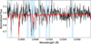 |
Fig. C.1 Same as Fig. 5 for NGC6822-55. Spectral lines Fe I λλ 11882.847 and Ti I λλ 11892.878 were excluded from the fit, because of artifact contamination. |
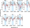 |
Fig. C.2 Same as Fig. 6, but for NGC6822-55. Spectral lines Fe I λλ 11882.847 and Ti I λλ 11892.878 were excluded from the fit, because of artifact contamination. |
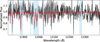 |
Fig. C.5 Same as Fig. 5, but for NGC6822-175. Spectral lines Si I λ 12103.54 and Mg I λ 12083.346 were excluded from the fit, because their profiles were too noisy. |
 |
Fig. C.6 Same as Fig. 6, but for NGC6822-175. Spectral lines Si I λ 12103.54 and Mg I λ 12083.346 were excluded from the fit, because their profiles were too noisy. |
 |
Fig. C.7 Same as Fig. 5, but for WLM 14. Spectral lines Fe I λλ 11882.847, Ti I λλ 11892.878 were excluded from the fit because of artifact contamination, and Si I λ 12103.54, was excluded because its profile was too noisy. |
 |
Fig. C.8 Same as Fig. 6, but for WLM 14. Spectral lines Fe I λλ 11882.847, Ti I λλ 11892.878 were excluded from the fit because of artifact contamination, and Si I λ 12103.54 was excluded because its profile was too noisy. |
Appendix D Light curves
This Appendix presents the optical, near-IR, and mid-IR light curves of the targets except for NGC6822-52, which was shown in the main text (Sect. 3.5). Symbols are described in Fig. 4.
 |
Fig. D.1 Same as Fig. 4, but for IC10-26089 (K4 I). For illustration purposes we show W1 + 4.0, W2 + 5.0. |
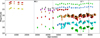 |
Fig. D.2 Same as Fig. 4, but for NGC6822-55. The gray dashed line denotes the epoch of the spectrum of Patrick et al. (2015). The spectral type of this object, both at the Levesque & Massey (2012) epoch and the OSIRIS epoch, is noted, highlighting its transition to warmer temperatures (see text for more details). |
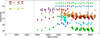 |
Fig. D.4 Same as Fig. 4, but for NGC6822-103. The gray solid line represents the epoch when the spectrum of Levesque & Massey (2012) was obtained. |
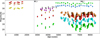 |
Fig. D.5 Same as Fig. 4, but for NGC6822-175. Lines are as in Fig. D.2. The spectral type of this object, both at the Levesque & Massey (2012) epoch and the OSIRIS epoch, is noted, marking its spectral variability. |
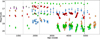 |
Fig. D.6 Same as Fig. 4, but for WLM 14 (K4-5 I). For illustration purposes we show W1 + 2.0, W2 + 3.0. The gray dashed line denotes the epoch when the data of Britavskiy et al. (2019) were obtained, while the gray dotted line indicates the epoch that the observations reported in Britavskiy et al. (2015) were carried out. |
Appendix E Periodograms
This Appendix provides the periodograms constructed for the 3 sources that display periodic behavior, namely NGC6822-52, WLM 14, and IC10-26089 (Sect. 4.2).
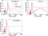 |
Fig. E.1 Periodograms of NGC6822-52 (top left), WLM 14 (top right) and IC10-26089 (bottom). The measured period is indicated by the black-dotted vertical line. |
All Tables
Parameters relevant to the fit carried out by MOLECFIT that are specific to EMIR.
All Figures
|
Fig. 1 Mid-IR (left) and near-IR (right) CMDs for the seven targets in NGC 6822, IC 10 and WLM. Red circles indicate targets whose spectra we were able to model. Background sources are stars from NGC 6822. The vertical line in the mid-IR CMD indicates the color criterion used for selecting stars with IR-excess. |
| In the text | |
|
Fig. 2 Spatial distribution of our targets in NGC 6822 and the targets of Patrick et al. (2015), two of which we have also observed. We included RSG candidates from the same work, one of which we have observed (see text for details). The background image is from the DSS2 survey. |
| In the text | |
|
Fig. 3 Revized spectral types of OSIRIS targets from de Wit et al. (2025), ordered in sequence of spectral type. Important spectral features are indicated. The spectrum and classification for WLM 14 are from Britavskiy et al. (2019). |
| In the text | |
|
Fig. 4 Light curve of NGC 6822-52. Filters and surveys are specified in the legend. Vertical lines indicate the epochs spectroscopy was obtained for this source. The dash-dotted line represents the epoch of our EMIR observations, while the dotted line denotes the epoch of the OSIRIS data (de Wit et al. 2025). |
| In the text | |
|
Fig. 5 Observed spectrum of NGC 6822-103 (in black) and best-fitting model (in red). The shaded blue regions highlight the spectral windows considered for the fitting process. The lines used for the fitting process from left to right by species are Fe I λλ 11 882.847, 11 973.050; Ti I λλ 11 892.878, 11 949.542; Si I λλ 11 984.20, 11 991.57, 12 031.50, 12 103.54, 12 270.50; Mg I λλ 11 828.185, 12083.346. |
| In the text | |
|
Fig. 6 Same as Fig. 5, but showing only the fitted spectral regions and the area around them. The contours represent the 68.3% confidence level errors. The spectral lines in each window are identified at the top of each panel. |
| In the text | |
|
Fig. 7 Cornerplot showing the samples from the posterior distribution of Teff, log g, [Fe/H], ξ, and radial velocity prior to the heliocentric correction (RV) for NGC 6822-103. The solution vector is (Teff, log g, [Fe/H], ξ, RV=(3845.23 K, 0.29, −0.54, 5.17 km s−1,−57.50 km s−1). Unfortunately, log g is not well constrained. Contours represent regions of highest posterior probability, and their shape highlights potential correlations. |
| In the text | |
|
Fig. 8 Zoom-in on the candidate-dimming event (marked with the dashed dotted lines) in the rZTF and W1-band light curves of NGC 6822-175. Possible locations of the minimum are highlighted with the shaded region. The dimming event of Betelgeuse is shown for comparison (gray triangles). Data were retrieved from the AAVSO database. |
| In the text | |
|
Fig. 9 HR diagram for targets with luminosity estimates. Red stars denote the |
| In the text | |
|
Fig. C.1 Same as Fig. 5 for NGC6822-55. Spectral lines Fe I λλ 11882.847 and Ti I λλ 11892.878 were excluded from the fit, because of artifact contamination. |
| In the text | |
|
Fig. C.2 Same as Fig. 6, but for NGC6822-55. Spectral lines Fe I λλ 11882.847 and Ti I λλ 11892.878 were excluded from the fit, because of artifact contamination. |
| In the text | |
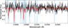 |
Fig. C.3 Same as Fig. 5, but for NGC6822-70. |
| In the text | |
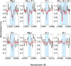 |
Fig. C.4 Same as Fig. 6, but for NGC6822-70. |
| In the text | |
|
Fig. C.5 Same as Fig. 5, but for NGC6822-175. Spectral lines Si I λ 12103.54 and Mg I λ 12083.346 were excluded from the fit, because their profiles were too noisy. |
| In the text | |
|
Fig. C.6 Same as Fig. 6, but for NGC6822-175. Spectral lines Si I λ 12103.54 and Mg I λ 12083.346 were excluded from the fit, because their profiles were too noisy. |
| In the text | |
|
Fig. C.7 Same as Fig. 5, but for WLM 14. Spectral lines Fe I λλ 11882.847, Ti I λλ 11892.878 were excluded from the fit because of artifact contamination, and Si I λ 12103.54, was excluded because its profile was too noisy. |
| In the text | |
|
Fig. C.8 Same as Fig. 6, but for WLM 14. Spectral lines Fe I λλ 11882.847, Ti I λλ 11892.878 were excluded from the fit because of artifact contamination, and Si I λ 12103.54 was excluded because its profile was too noisy. |
| In the text | |
|
Fig. D.1 Same as Fig. 4, but for IC10-26089 (K4 I). For illustration purposes we show W1 + 4.0, W2 + 5.0. |
| In the text | |
|
Fig. D.2 Same as Fig. 4, but for NGC6822-55. The gray dashed line denotes the epoch of the spectrum of Patrick et al. (2015). The spectral type of this object, both at the Levesque & Massey (2012) epoch and the OSIRIS epoch, is noted, highlighting its transition to warmer temperatures (see text for more details). |
| In the text | |
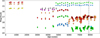 |
Fig. D.3 Same as Fig. 4, but for NGC6822-70. |
| In the text | |
|
Fig. D.4 Same as Fig. 4, but for NGC6822-103. The gray solid line represents the epoch when the spectrum of Levesque & Massey (2012) was obtained. |
| In the text | |
|
Fig. D.5 Same as Fig. 4, but for NGC6822-175. Lines are as in Fig. D.2. The spectral type of this object, both at the Levesque & Massey (2012) epoch and the OSIRIS epoch, is noted, marking its spectral variability. |
| In the text | |
|
Fig. D.6 Same as Fig. 4, but for WLM 14 (K4-5 I). For illustration purposes we show W1 + 2.0, W2 + 3.0. The gray dashed line denotes the epoch when the data of Britavskiy et al. (2019) were obtained, while the gray dotted line indicates the epoch that the observations reported in Britavskiy et al. (2015) were carried out. |
| In the text | |
|
Fig. E.1 Periodograms of NGC6822-52 (top left), WLM 14 (top right) and IC10-26089 (bottom). The measured period is indicated by the black-dotted vertical line. |
| In the text | |
Current usage metrics show cumulative count of Article Views (full-text article views including HTML views, PDF and ePub downloads, according to the available data) and Abstracts Views on Vision4Press platform.
Data correspond to usage on the plateform after 2015. The current usage metrics is available 48-96 hours after online publication and is updated daily on week days.
Initial download of the metrics may take a while.