| Issue |
A&A
Volume 704, December 2025
|
|
|---|---|---|
| Article Number | A116 | |
| Number of page(s) | 9 | |
| Section | Galactic structure, stellar clusters and populations | |
| DOI | https://doi.org/10.1051/0004-6361/202554276 | |
| Published online | 09 December 2025 | |
The dependence of black-hole formation in open clusters on the cluster formation process
Max-Planck-Institut für Radioastronomie,
Auf dem Hügel 69,
53121
Bonn,
Germany
★ Corresponding author: This email address is being protected from spambots. You need JavaScript enabled to view it.
Received:
26
February
2025
Accepted:
15
October
2025
Abstract
We performed N-body simulations of both individual cluster evolution and subcluster coalescence, demonstrating that cluster evolution and its outcomes strongly depend on the cluster formation process through comparisons of different gas expulsion modes and formation channels. The evolution of star clusters is significantly shaped by the gas expulsion mode, with faster expulsion producing greater mass loss. A broader degeneracy exists among initial cluster mass, gas expulsion timescale, and formation channel (monolithic vs. coalescence), which manifests in both evolutionary pathways and black-hole production. In individual cluster simulations, slower gas expulsion enables progressively lower mass clusters to retain central black holes within the tidal radius. As the gas expulsion mode transitions from fast to moderate to slow, the fraction of high-velocity stars decreases. Variations in gas expulsion mode and formation channel ultimately influence the stellar velocity distribution (within the tidal radius) and, thus, the expansion speed, which governs both cluster mass loss and black-hole retention. Slowly expanding clusters are more likely to retain black holes and multiple systems, making them prime candidates for black-hole searches with Gaia. Our results highlight the crucial influence of early gas expulsion and cluster formation mechanisms on the dynamical evolution of star clusters and black-hole production. These factors should be carefully incorporated into the initial conditions of N-body simulations, which necessarily rely on input from the star formation community.
Key words: stars: black holes / stars: evolution / ISM: clouds / open clusters and associations: general
© The Authors 2025
 Open Access article, published by EDP Sciences, under the terms of the Creative Commons Attribution License (https://creativecommons.org/licenses/by/4.0), which permits unrestricted use, distribution, and reproduction in any medium, provided the original work is properly cited.
This article is published in open access under the Subscribe to Open model.
Open Access funding provided by Max Planck Society.
1 Introduction
Recent proper motion data from Gaia’s data release 3 (DR3; Gaia Collaboration 2023) have led to the discovery of two dormant black holes (BHs; i.e., Gaia BH1 and Gaia BH2) in BH–star binary systems within the Galactic field (Chakrabarti et al. 2023; El-Badry et al. 2023b,a; Tanikawa et al. 2023). As part of the validation process for the upcoming fourth Gaia data release (DR4), Gaia Collaboration (2024) analyzed preliminary astrometric binary solutions and identified a black hole with a mass of ∼33 M⊙ in a binary system, now referred to as Gaia BH3. Following the detection of Gaia BH1 and Gaia BH2, discussions and hypotheses emerged regarding the origins of these systems. The formation histories of Gaia BH1 and Gaia BH2 are challenging to reconcile with isolated binary (IB) evolution, as their orbital properties do not align with the expected outcomes of common envelope evolution (El-Badry et al. 2023a,b). Their near-solar metallicities and inferred orbits within the Galactic plane suggest that they were likely formed in open clusters (Rastello et al. 2023; Di Carlo et al. 2024; Marín Pina et al. 2024; Tanikawa et al. 2024).
Young and open star clusters host most massive stars, which are the precursors of compact objects. Consequently, the majority of black holes in the Milky Way likely spent their early years in these clusters, engaging in dynamic interactions. N-body simulations are powerful tools for studying star cluster dynamics and black-hole formation within clusters. Physically, the initial conditions of N-body simulations are determined by the star-cluster formation process. Given the significant progress in observational studies of massive-star and star-cluster formation (Motte et al. 2018; Beuther et al. 2025), these observational results should be translated into the initial conditions for star-cluster dynamical simulations (see Appendix A for more details). This work also examined how initial conditions and the cluster formation process influence the evolutionary outcomes of star clusters.
2 N-body simulations
A portion of the N-body simulations for star clusters presented in Zhou et al. (2024b, 2025b,a) are summarized in Table 1. The detailed simulation setups are also thoroughly documented in these studies. For the convenience of the reader, these setups are summarized again in Appendix A. These simulations were previously employed to explain the observed physical parameters of open clusters. In this work, however, we focused on the final products of these simulations, i.e., black holes. Overall, the simulations can be divided into two categories: the cluster-coalescence simulations (Zhou et al. 2025b) and the individual cluster simulations (Zhou et al. 2024b); these are labeled as “individual” and “coalescence” in Table 1. As described in Appendix A, for individual clusters, we simulated four gas-expulsion modes (fast, moderate2/mod2, moderate1/mod1, and slow), characterized by gas-expulsion timescales of τg, 2τg, 5τg, and 10τg, respectively. To mitigate the stochasticity of the simulation results, we further refined the mass grid and simulated additional clusters using the same setups. All new simulations (i.e., except those listed in Table 1) were evolved until 100 Myr in order to reduce computational costs. Finally, the simulated cluster masses are [300, 562, 1000, 1333, 1778, 2371, 3000, 5623, and 10 000] M⊙, corresponding to [102.5, 102.75, 103, 103.125, 103.25, 103.375, 103.5, 103.75, 104] M⊙. For the cluster complex NGC6334 in the coalescence simulations, each subcluster adopts the fast gas-expulsion mode. As described in Appendix A, we considered two scenarios: (i) all subclusters are initially at rest and located in the same plane (“-fast”); and (ii) the subclusters are spatially separated and possess velocity differences (“-fast-vd”).
N-body simulations of subcluster coalescence and cluster evolution under different gas expulsion modes.
3 Results and discussion
3.1 Cluster evolution
The evolution of clusters under different simulation scenarios has been extensively analyzed in Zhou et al. (2024b, 2025b,a). Here we summarize several key conclusions. For individual cluster simulations, the extent of cluster mass loss is strongly governed by the gas expulsion mode: the faster the gas expulsion, the greater the mass loss. However, there exists a degeneracy between cluster mass and gas expulsion timescale. For example, a massive cluster undergoing fast gas expulsion expands rapidly and loses mass at a high rate, whereas a lower mass cluster experiencing slow gas expulsion evolves more gradually, resulting in slower mass loss. Consequently, clusters with different initial masses and gas-expulsion timescales may display similar evolutionary outcomes. As shown in Fig. 1a, a 1000 M⊙ cluster with slow gas expulsion evolves similarly to a 3000 M⊙ cluster with moderate gas expulsion. Conversely, a 10 000 M⊙ cluster with fast gas expulsion exhibits evolutionary behaviour comparable to that of a 3000 M⊙ cluster with moderate gas expulsion. In cluster coalescence simulations, the spatial distribution, relative velocities, mass distribution, and gas expulsion modes of subclusters jointly influence both the dynamics of the merging process and the stability of the final product. As shown in Fig. 1b, although each subcluster undergoes fast gas expulsion, the evolution of the merged cluster closely resembles that of a single cluster with moderate gas expulsion in the individual cluster simulations. These findings highlight a degeneracy among cluster mass, gas expulsion mode, and the cluster formation channel (i.e., monolithic versus coalescence).
3.2 Black-hole production
The degeneracy between cluster mass and the initial gas-expulsion mode is also reflected in the eventual black-hole production of star clusters, as shown in Fig. 2. For individual cluster simulations, under fast gas expulsion, only the most massive cluster (10 000 M⊙) can retain black holes within the tidal radius for extended periods. As the gas-expulsion mode transitions from fast to moderate and then to slow, progressively lower mass clusters are able to retain black holes within the tidal radius, and the number of retained black holes also increases. When the gas-expulsion mode changes from “fast” (τg) to “moderate2” (2τg), the timescale itself changes only slightly; however, the subsequent cluster evolution and final outcome differ substantially. This underscores the importance of carefully constraining the initial conditions of N-body simulations of cluster evolution (see Sect. 3.3 for further discussion).
In cluster-coalescence simulations (Fig. 3), although each initial subcluster undergoes fast gas expulsion, the merged cluster with a initial mass of 2207 M⊙ can still retain a black hole within the tidal radius. This again reflects the degeneracy between cluster mass and the cluster formation mechanism. However, coalescence simulations are far more complex than individual cluster simulations, involving a rich parameter space that remains to be explored. This work only illustrates the signifi-cant differences between cluster coalescence and the evolution of a single cluster by comparing a cluster complex (NGC6334) with a single cluster (2371 M⊙) of similar mass, rather than providing a detailed discussion of cluster coalescence itself.
Figure 5 shows the velocity distribution of stars in the cluster complex NGC6334 and in the 2371 M⊙ cluster under different gas-expulsion modes. As the gas-expulsion mode transitions from fast to moderate to slow, the fraction of high-velocity stars in the cluster decreases. In contrast, for the cluster complex, despite each subcluster undergoing fast gas expulsion, the velocity distribution of the coalesced cluster is significantly lower overall. The stellar velocity distribution of a star cluster reflects its expansion speed, which plays a crucial role in determining whether massive stars and their remnants remain bound. Variations in cluster mass, gas expulsion mode, and formation mechanism ultimately influence the cluster expansion speed, which in turn affects both the mass-loss rate and the rate of black-hole formation.
In Fig. 4, closely spaced black holes are shown. Their ability to form multiple systems (binary or triple) also depends on the dynamical state of the cluster. The initial gas expulsion mode is critical to the cluster’s dynamical evolution and has a strong impact on its lifetime. Black holes in slowly expanding clusters experience a more stable dynamical environment and thus have significantly more time to evolve within the system. The number of central black holes in Figs. 4a and b are two and three, respectively. Fig. 6 illustrates the time evolution of the separations between each pair of black holes. The three black holes in Fig. 4b eventually form a triple system, whereas the two black holes in Fig. 4a fail to form a binary, even by the time the cluster dissolves.
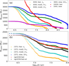 |
Fig. 1 Evolution of cluster mass over time under different gas expulsion modes. In panel b, the total mass of the cluster complex “NGC6334” is 2207 M⊙, which is close to the single cluster witha mass of 2371 M⊙. Here, we only consider the total cluster mass within the tidal radius. |
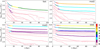 |
Fig. 2 Evolution of cluster mass over time under different gas expulsion modes. The color of the line reflects the number of black holes contained in a cluster of a given mass at a certain age. Here, we only consider the total cluster mass and the number of black holes within the tidal radius. For each panel, from bottom to top, the cluster masses are [300, 562, 1000, 1333, 1778, 2371, 3000, 5623, and 10 000] M⊙. |
3.3 Gas-expulsion mode
In the above analysis, we demonstrate the crucial influence of the gas-expulsion mode and cluster formation mechanism on the dynamical evolution of star clusters and black-hole production. Therefore, these factors should be carefully incorporated into the initial conditions of N-body simulations.
Giant molecular clouds (GMCs) are widely recognized as the primary gas reservoirs fueling star formation and serving as the birthplaces of nearly all stars. Within these clouds, clumps are dense, localized structures that act as the main sites of star formation (Urquhart et al. 2018, 2022). The process of star cluster formation in molecular clouds involves several stages: the formation of clumps in diffuse gas, the evolution of these clumps, the emergence of embedded clusters within them, and the subsequent evolution of the embedded clusters alongside clump dispersal driven by feedback (Krumholz et al. 2019; Krause et al. 2020; Zhou et al. 2022, Zhou et al. 2024d). In Urquhart et al. (2018, 2022), the ATLASGAL clumps at various evolutionary stages encompass all of these physical processes. Eventually, a clump forms an embedded cluster with an IMF (Yan et al. 2017; Zhou et al. 2024e,c). An ATLASGAL clump associated with an HII region (HII-clump) consists of an embedded cluster surrounded by a gas envelope, with residual gas remaining inside the cluster. High-resolution Atacama Large Millimeter/submillimeter Array (ALMA) observations of HII-clumps presented in Zhou et al. (2024d) reveal distinct gas shells enclosing the protoclusters. HII-clumps represent the final stage of embedded cluster formation within clumps. They are critical for bridging the stellar-kinematics and abundance community with the star formation community, as protoclusters or embedded clusters in HII-clumps mark the earliest stage of gas-free star clusters.
Following gas expulsion driven by feedback from the embedded cluster, the cluster undergoes expansion (Kuhn et al. 2019; Wright et al. 2024; Della Croce et al. 2024; Zhou et al. 2024g). Understanding the detailed feedback processes within clumps is essential for tracing the evolutionary pathway from clumps to embedded clusters, and ultimately opening clusters, and thus it is vital for setting the initial conditions of N-body simulations. The strength of feedback depends on the mass of the embedded cluster, leading to variations in the gas-expulsion timescale. More massive clumps give rise to more massive clusters, which, in turn, generate stronger feedback and higher gas-expulsion velocities (Dib et al. 2013; Zhou et al. 2024c). A correlation is therefore expected between feedback strength, clump (or embedded cluster) mass, and gas expulsion velocity. Low-mass clusters are expected to undergo slower gas expulsion compared to high-mass clusters (Pang et al. 2021). Moreover (as discussed in Appendix A), beyond feedback strength, uncertainties in the star formation efficiency, the geometric shape of the gas shell, and the external gas potential can also be incorporated into the gas-expulsion timescale. Therefore, integrating both hydrodynamics and N-body simulations is crucial for advancing our understanding of early cluster feedback and gas-expulsion processes in HII-clumps, as well as for quantifying the impact of the aforementioned factors on the gas expulsion timescale (Sills et al. 2018; Suin et al. 2022; Rieder et al. 2022; Fujii et al. 2022; Lewis et al. 2023; Cournoyer-Cloutier et al. 2023; Rodriguez et al. 2023; Jo et al. 2024; Polak et al. 2024).
In Zhou et al. (2025c), we attempted to constrain the gas expulsion mode of initially embedded clusters by inversely analyzing the expansion speed of very young open clusters (<5 Myr) using Gaia DR3 data. By comparing with N-body simulations, we found that all gas expulsion modes (fast, moderate, slow) remain possible. As discussed in Sect. 3.2, slowly expanding clusters are more likely to retain black holes and black-hole multiple systems, making them promising candidates for black-hole searches with Gaia observations.
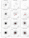 |
Fig. 4 Evolution of 3000 M⊙ cluster under different gas-expulsion modes. Snapshots projected on the XY plane (20 pc × 20 pc around the cluster center) at ages 10 Myr, 50 Myr, and 100 Myr are shown here. The size of the black dots reflects the stellar mass (linear scale). Neutron stars and black holes are represented by orange plus signs and red dots, respectively, with the symbol sizes being purely illustrative. The central regions of the star clusters in Figs. 4a and b contain two and three black holes, respectively. In panel b, two of the three black holes are too close to be distinguished on the map. |
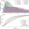 |
Fig. 5 Velocity distribution of stars within cluster complex “NGC6334” and 2371 M⊙ cluster under different gas-expulsion modes at 20 Myr. (a) Probability density function (PDF) of stellar velocities, estimated using the kernel-density-estimation (KDE) method to provide a smooth representation of the distribution; (b) cumulative fraction shows the proportion of stars with velocities below a given value. Here, we do not distinguish between binaries and single stars; instead, we calculated the total velocity of each star (vtot) in the cluster and examined their distribution to roughly characterize the expansion state of the cluster. At 50 Myr, the velocity distributions remain unchanged, indicating that the binary fraction does not significantly affect the statistical results here. |
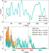 |
Fig. 6 Temporal evolution of distance between each pair of black holes. Panels a and b correspond to black-hole pairs in panels a and b of Fig. 4, respectively. |
3.4 Cluster formation mechanism
In Zhou et al. (2024c), we collected samples of Galactic clumps, embedded clusters, and open clusters to compare their physical properties. We showed that the mass distribution of open clusters spans a significantly broader range than that of embedded clusters, by about one order of magnitude. Given the present-day mass distribution of clumps in the Milky Way, the simple evolutionary sequence of a single clump evolving into an embedded cluster and subsequently into an open cluster cannot account for the observed old and massive open clusters. This conclusion is also supported by N-body simulations of individual embedded clusters. Furthermore, we compared the separations of open clusters with the typical sizes of molecular clouds in the Milky Way and found that most molecular clouds are likely to form only one open cluster. Since a molecular cloud generally produces many embedded clusters, this result supports the coalescence scenario. The typical separation between embedded clusters in massive star-forming regions can be ≈1 pc (Zhou et al. 2024f). Therefore, after expansion, these clusters are expected to undergo coalescence. There is now extensive literature suggesting that star clusters form through the merging of subclusters, supported by both simulations (Vázquez-Semadeni et al. 2009; Fujii et al. 2012; Vázquez-Semadeni et al. 2017; Howard et al. 2018; Sills et al. 2018; Fujii et al. 2022; Dobbs et al. 2022; Guszejnov et al. 2022; Cournoyer-Cloutier et al. 2023; Polak et al. 2024) and observations (Sabbi et al. 2012; Dalessandro et al. 2021; Pang et al. 2022; Della Croce et al. 2023; Fahrion & De Marchi 2024). Building on the work of Zhou et al. (2024b), Zhou et al. (2025b) explored a scenario in which open clusters form via post-gas-expulsion coalescence of embedded clusters within the same parental molecular cloud and found that the merging of multiple low-mass embedded clusters can reproduce the observed parameter space of open clusters in the Milky Way.
In the cluster coalescence and individual cluster simulations of Zhou et al. (2024b, 2025b,a), the dynamical states of coalesced and single-star clusters differ substantially throughout their evolution, leading to distinct outcomes, as also discussed above. Since embedded cluster coalescence is a key pathway for open cluster formation, investigating black-hole formation across diverse coalescence scenarios is particularly promising. In coalescence scenarios, cluster dynamics and black-hole formation are influenced by multiple factors, including the mass ratio, spatial separation, relative velocity, collision angle, and initial expansion speed of the subclusters. Possible coalescence scenarios may be inferred from massive star-forming regions in the Milky Way.
Since we adhered to the mmax–Mecl relation in all simulations, cluster complexes and single clusters with similar total masses contain significantly different numbers of massive stars, which may in turn have a substantial impact on final black-hole production. However, the mmax–Mecl relation has mainly been tested for individual embedded clusters (Weidner et al. 2013; Zhou et al. 2024c), and whether it also applies to cluster complexes and their subclusters requires further observational verification.
4 Conclusion
The evolution of star clusters is significantly influenced by the gas expulsion mode, with faster expulsion leading to greater mass loss. However, a degeneracy exists whereby clusters of different initial masses (e.g., 1000 M⊙ with slow expulsion and 3000 M⊙ with moderate expulsion) can follow similar evolutionary pathways. In coalescence scenarios, despite subclusters undergoing fast expulsion, the resulting merged cluster can resemble a single cluster with moderate expulsion. This highlights a broader degeneracy between initial cluster mass, gas expulsion timescale, and cluster formation channel (monolithic vs. coalescence).
This degeneracy also plays a key role in black-hole retention and dynamical evolution. In individual cluster simulations, slower gas expulsion allows progressively lower mass clusters to retain central black holes, while in coalescence simulations even a 2207 M⊙ coalesced cluster can retain one despite fast gas expulsion. Variations in gas expulsion mode and formation channel ultimately influence the stellar velocity distribution (within the tidal radius), and thus the expansion speed, which governs both cluster mass loss and black-hole retention. As the gas-expulsion mode transitions from fast to moderate to slow, the fraction of high-velocity stars in the cluster decreases. In contrast, for the cluster complex, despite each subcluster undergoing fast gas expulsion, the velocity distribution of the coalesced cluster is significantly lower overall. The number and configuration of retained black holes (binary or triple systems) depend sensitively on the cluster’s dynamical state, which is itself strongly shaped by the initial gas expulsion mode. Since slowly expanding clusters are more likely to retain black holes and multiple systems, making them prime candidates for black-hole searches with Gaia.
Giant molecular clouds (GMCs) host dense clumps as the primary sites of star formation, evolving through stages that culminate in embedded clusters surrounded by gas envelopes, as seen in ATLASGAL HII-clumps. The subsequent gas expulsion, driven by feedback whose strength correlates with cluster mass, critically determines the cluster’s expansion. This process, influenced by factors such as star formation efficiency and gas geometry, sets the initial conditions for N-body simulations. Integrating hydrodynamic and N-body simulations is essential for constraining early feedback and gas expulsion in HII-clumps.
In coalescence scenarios, cluster dynamics and black hole formation are influenced by multiple factors, including the mass ratio, spatial separation, relative velocity, collision angle, and initial expansion speed of the subclusters. Since embedded cluster coalescence is a key pathway for open cluster formation, investigating black-hole formation across diverse coalescence scenarios is particularly promising. Adherence to the mmax–Mecl relation in both individual and coalescence simulations implies that cluster complexes and single clusters of similar total mass contain different numbers of massive stars, which may significantly impact final black-hole production, although the applicability of this relation to cluster complexes and their subclusters requires further observational verification.
Acknowledgements
Thanks to the referee for the detailed and constructive comments, which have significantly contributed to improving this work.
References
- Aarseth, S. J., Henon, M., & Wielen, R. 1974, A&A, 37, 183 [NASA ADS] [Google Scholar]
- Alfaro, E. J., & Román-Zúñiga, C. G. 2018, MNRAS, 478, L110 [Google Scholar]
- André, P. J., Palmeirim, P., & Arzoumanian, D. 2022, A&A, 667, L1 [CrossRef] [EDP Sciences] [Google Scholar]
- Banerjee, S., & Kroupa, P. 2013, ApJ, 764, 29 [CrossRef] [Google Scholar]
- Banerjee, S., & Kroupa, P. 2014, ApJ, 787, 158 [NASA ADS] [CrossRef] [Google Scholar]
- Banerjee, S., & Kroupa, P. 2015, MNRAS, 447, 728 [NASA ADS] [CrossRef] [Google Scholar]
- Banerjee, S., & Kroupa, P. 2017, A&A, 597, A28 [NASA ADS] [CrossRef] [EDP Sciences] [Google Scholar]
- Banerjee, S., Kroupa, P., & Oh, S. 2012, ApJ, 746, 15 [Google Scholar]
- Banerjee, S., Belczynski, K., Fryer, C. L., et al. 2020, A&A, 639, A41 [NASA ADS] [CrossRef] [EDP Sciences] [Google Scholar]
- Bate, M. R., Tricco, T. S., & Price, D. J. 2014, MNRAS, 437, 77 [NASA ADS] [CrossRef] [Google Scholar]
- Baumgardt, H., & Kroupa, P. 2007, MNRAS, 380, 1589 [NASA ADS] [CrossRef] [Google Scholar]
- Belloni, D., Askar, A., Giersz, M., Kroupa, P., & Rocha-Pinto, H. J. 2017, MNRAS, 471, 2812 [NASA ADS] [CrossRef] [Google Scholar]
- Beuther, H., Kuiper, R., & Tafalla, M. 2025, A&A, 63, 1 [Google Scholar]
- Brinkmann, N., Banerjee, S., Motwani, B., & Kroupa, P. 2017, A&A, 600, A49 [NASA ADS] [CrossRef] [EDP Sciences] [Google Scholar]
- Chakrabarti, S., Simon, J. D., Craig, P. A., et al. 2023, AJ, 166, 6 [NASA ADS] [CrossRef] [Google Scholar]
- Chen, L., de Grijs, R., & Zhao, J. L. 2007, AJ, 134, 1368 [NASA ADS] [CrossRef] [Google Scholar]
- Cournoyer-Cloutier, C., Sills, A., Harris, W. E., et al. 2023, MNRAS, 521, 1338 [NASA ADS] [CrossRef] [Google Scholar]
- Dalessandro, E., Varri, A. L., Tiongco, M., et al. 2021, ApJ, 909, 90 [NASA ADS] [CrossRef] [Google Scholar]
- Della Croce, A., Dalessandro, E., Livernois, A., et al. 2023, A&A, 674, A93 [NASA ADS] [CrossRef] [EDP Sciences] [Google Scholar]
- Della Croce, A., Dalessandro, E., Livernois, A., & Vesperini, E. 2024, A&A, 683, A10 [NASA ADS] [CrossRef] [EDP Sciences] [Google Scholar]
- Di Carlo, U. N., Agrawal, P., Rodriguez, C. L., & Breivik, K. 2024, ApJ, 965, 22 [CrossRef] [Google Scholar]
- Dib, S., Gutkin, J., Brandner, W., & Basu, S. 2013, MNRAS, 436, 3727 [NASA ADS] [CrossRef] [Google Scholar]
- Dinnbier, F., Kroupa, P., & Anderson, R. I. 2022, A&A, 660, A61 [NASA ADS] [CrossRef] [EDP Sciences] [Google Scholar]
- Dobbs, C. L., Bending, T. J. R., Pettitt, A. R., Buckner, A. S. M., & Bate, M. R. 2022, MNRAS, 517, 675 [NASA ADS] [CrossRef] [Google Scholar]
- El-Badry, K., Rix, H.-W., Cendes, Y., et al. 2023a, MNRAS, 521, 4323 [NASA ADS] [CrossRef] [Google Scholar]
- El-Badry, K., Rix, H.-W., Quataert, E., et al. 2023b, MNRAS, 518, 1057 [Google Scholar]
- Fahrion, K., & De Marchi, G. 2024, A&A, 681, A20 [NASA ADS] [CrossRef] [EDP Sciences] [Google Scholar]
- Farias, J. P., Offner, S. S. R., Grudić, M. Y., Guszejnov, D., & Rosen, A. L. 2024, MNRAS, 527, 6732 [Google Scholar]
- Fujii, M. S., Saitoh, T. R., & Portegies Zwart, S. F. 2012, ApJ, 753, 85 [NASA ADS] [CrossRef] [Google Scholar]
- Fujii, M. S., Wang, L., Hirai, Y., et al. 2022, MNRAS, 514, 2513 [NASA ADS] [CrossRef] [Google Scholar]
- Gaia Collaboration (Vallenari, A., et al.) 2023, A&A, 674, A1 [NASA ADS] [CrossRef] [EDP Sciences] [Google Scholar]
- Gaia Collaboration (Panuzzo, P., et al.) 2024, A&A, 686, L2 [NASA ADS] [CrossRef] [EDP Sciences] [Google Scholar]
- Getman, K. V., Feigelson, E. D., Kuhn, M. A., et al. 2014, ApJ, 787, 108 [Google Scholar]
- Geyer, M. P., & Burkert, A. 2001, MNRAS, 323, 988 [NASA ADS] [CrossRef] [Google Scholar]
- Giacobbo, N., Mapelli, M., & Spera, M. 2018, MNRAS, 474, 2959 [Google Scholar]
- Guszejnov, D., Markey, C., Offner, S. S. R., et al. 2022, MNRAS, 515, 167 [NASA ADS] [CrossRef] [Google Scholar]
- Heggie, D., & Hut, P. 2003, The Gravitational Million-Body Problem: A Multidisciplinary Approach to Star Cluster Dynamics [Google Scholar]
- Howard, C. S., Pudritz, R. E., & Harris, W. E. 2018, Nat. Astron., 2, 725 [NASA ADS] [CrossRef] [Google Scholar]
- Hurley, J. R., Pols, O. R., & Tout, C. A. 2000, MNRAS, 315, 543 [Google Scholar]
- Hurley, J. R., Tout, C. A., & Pols, O. R. 2002, MNRAS, 329, 897 [Google Scholar]
- Jo, Y., Kim, S., Kim, J.-h., & Bryan, G. L. 2024, ApJ, 974, 193 [Google Scholar]
- Kirk, H., & Myers, P. C. 2011, ApJ, 727, 64 [Google Scholar]
- Krause, M. G. H., Offner, S. S. R., Charbonnel, C., et al. 2020, Space Sci. Rev., 216, 64 [CrossRef] [Google Scholar]
- Kroupa, P. 1995a, MNRAS, 277, 1491 [Google Scholar]
- Kroupa, P. 1995b, MNRAS, 277, 1507 [NASA ADS] [Google Scholar]
- Kroupa, P. 2001, MNRAS, 322, 231 [NASA ADS] [CrossRef] [Google Scholar]
- Kroupa, P. 2008, in The Cambridge N-Body Lectures, 760, eds. S.J. Aarseth, C.A. Tout, & R.A. Mardling, 181 [Google Scholar]
- Kroupa, P., Aarseth, S., & Hurley, J. 2001, MNRAS, 321, 699 [NASA ADS] [CrossRef] [Google Scholar]
- Krumholz, M. R., McKee, C. F., & Bland-Hawthorn, J. 2019, A&A, 57, 227 [Google Scholar]
- Kuhn, M. A., Hillenbrand, L. A., Sills, A., Feigelson, E. D., & Getman, K. V. 2019, ApJ, 870, 32 [CrossRef] [Google Scholar]
- Kumar, M. S. N., Palmeirim, P., Arzoumanian, D., & Inutsuka, S. I. 2020, A&A, 642, A87 [EDP Sciences] [Google Scholar]
- Küpper, A. H. W., Maschberger, T., Kroupa, P., & Baumgardt, H. 2011, MNRAS, 417, 2300 [Google Scholar]
- Lada, C. J., & Lada, E. A. 2003, A&A, 41, 57 [Google Scholar]
- Lane, J., Kirk, H., Johnstone, D., et al. 2016, ApJ, 833, 44 [Google Scholar]
- Lewis, S. C., McMillan, S. L. W., Low, M.-M. M., et al. 2023, ApJ, 944, 211 [NASA ADS] [CrossRef] [Google Scholar]
- Littlefair, S. P., Naylor, T., Jeffries, R. D., Devey, C. R., & Vine, S. 2003, MNRAS, 345, 1205 [NASA ADS] [CrossRef] [Google Scholar]
- Machida, M. N., & Matsumoto, T. 2012, MNRAS, 421, 588 [NASA ADS] [Google Scholar]
- Malinen, J., Juvela, M., Rawlings, M. G., et al. 2012, A&A, 544, A50 [NASA ADS] [CrossRef] [EDP Sciences] [Google Scholar]
- Marín Pina, D., Rastello, S., Gieles, M., et al. 2024, A&A, 688, L2 [NASA ADS] [CrossRef] [EDP Sciences] [Google Scholar]
- Marks, M., & Kroupa, P. 2012, A&A, 543, A8 [NASA ADS] [CrossRef] [EDP Sciences] [Google Scholar]
- Megeath, S. T., Gutermuth, R., Muzerolle, J., et al. 2016, AJ, 151, 5 [Google Scholar]
- Motte, F., Bontemps, S., & Louvet, F. 2018, A&A, 56, 41 [Google Scholar]
- Nony, T., Robitaille, J. F., Motte, F., et al. 2021, A&A, 645, A94 [NASA ADS] [CrossRef] [EDP Sciences] [Google Scholar]
- Oh, S., & Kroupa, P. 2016, A&A, 590, A107 [NASA ADS] [CrossRef] [EDP Sciences] [Google Scholar]
- Oh, S., & Kroupa, P. 2018, MNRAS, 481, 153 [NASA ADS] [CrossRef] [Google Scholar]
- Oh, S., Kroupa, P., & Pflamm-Altenburg, J. 2015, ApJ, 805, 92 [Google Scholar]
- Pang, X., Li, Y., Yu, Z., et al. 2021, ApJ, 912, 162 [NASA ADS] [CrossRef] [Google Scholar]
- Pang, X., Tang, S.-Y., Li, Y., et al. 2022, ApJ, 931, 156 [NASA ADS] [CrossRef] [Google Scholar]
- Pavlik, V., Kroupa, P., & Šubr, L. 2019, A&A, 626, A79 [NASA ADS] [CrossRef] [EDP Sciences] [Google Scholar]
- Plunkett, A. L., Fernández-López, M., Arce, H. G., et al. 2018, A&A, 615, A9 [NASA ADS] [CrossRef] [EDP Sciences] [Google Scholar]
- Polak, B., Mac Low, M.-M., Klessen, R. S., et al. 2024, A&A, 690, A207 [NASA ADS] [CrossRef] [EDP Sciences] [Google Scholar]
- Portegies Zwart, S. F., McMillan, S. L. W., & Gieles, M. 2010, A&A, 48, 431 [Google Scholar]
- Rahner, D., Pellegrini, E. W., Glover, S. C. O., & Klessen, R. S. 2017, MNRAS, 470, 4453 [NASA ADS] [CrossRef] [Google Scholar]
- Rastello, S., Iorio, G., Mapelli, M., et al. 2023, MNRAS, 526, 740 [NASA ADS] [CrossRef] [Google Scholar]
- Rieder, S., Dobbs, C., Bending, T., Liow, K. Y., & Wurster, J. 2022, MNRAS, 509, 6155 [Google Scholar]
- Rodriguez, C. L., Hafen, Z., Grudić, M. Y., et al. 2023, MNRAS, 521, 124 [CrossRef] [Google Scholar]
- Röser, S., & Schilbach, E. 2019, A&A, 627, A4 [NASA ADS] [CrossRef] [EDP Sciences] [Google Scholar]
- Röser, S., Schilbach, E., Piskunov, A. E., Kharchenko, N. V., & Scholz, R. D. 2011, A&A, 531, A92 [NASA ADS] [CrossRef] [EDP Sciences] [Google Scholar]
- Sabbi, E., Lennon, D. J., Gieles, M., et al. 2012, ApJ, 754, L37 [Google Scholar]
- Sana, H., de Mink, S. E., de Koter, A., et al. 2012, Science, 337, 444 [Google Scholar]
- Sills, A., Rieder, S., Scora, J., McCloskey, J., & Jaffa, S. 2018, MNRAS, 477, 1903 [Google Scholar]
- Suin, P., Shore, S. N., & Pavlík, V. 2022, A&A, 667, A69 [NASA ADS] [CrossRef] [EDP Sciences] [Google Scholar]
- Tanikawa, A., Yoshida, T., Kinugawa, T., Takahashi, K., & Umeda, H. 2020, MNRAS, 495, 4170 [NASA ADS] [CrossRef] [Google Scholar]
- Tanikawa, A., Hattori, K., Kawanaka, N., et al. 2023, ApJ, 946, 79 [CrossRef] [Google Scholar]
- Tanikawa, A., Cary, S., Shikauchi, M., Wang, L., & Fujii, M. S. 2024, MNRAS, 527, 4031 [Google Scholar]
- Urquhart, J. S., König, C., Giannetti, A., et al. 2018, MNRAS, 473, 1059 [Google Scholar]
- Urquhart, J. S., Wells, M. R. A., Pillai, T., et al. 2022, MNRAS, 510, 3389 [NASA ADS] [CrossRef] [Google Scholar]
- Vázquez-Semadeni, E., Gómez, G. C., Jappsen, A. K., Ballesteros-Paredes, J., & Klessen, R. S. 2009, ApJ, 707, 1023 [CrossRef] [Google Scholar]
- Vázquez-Semadeni, E., González-Samaniego, A., & Colín, P. 2017, MNRAS, 467, 1313 [NASA ADS] [Google Scholar]
- Vázquez-Semadeni, E., Palau, A., Ballesteros-Paredes, J., Gómez, G. C., & Zamora-Avilés, M. 2019, MNRAS, 490, 3061 [Google Scholar]
- von Steiger, R., & Zurbuchen, T. H. 2016, ApJ, 816, 13 [Google Scholar]
- Wang, L., Kroupa, P., & Jerabkova, T. 2019, MNRAS, 484, 1843 [NASA ADS] [CrossRef] [Google Scholar]
- Wang, L., Iwasawa, M., Nitadori, K., & Makino, J. 2020, MNRAS, 497, 536 [NASA ADS] [CrossRef] [Google Scholar]
- Weidner, C., Kroupa, P., & Pflamm-Altenburg, J. 2013, MNRAS, 434, 84 [NASA ADS] [CrossRef] [Google Scholar]
- Wright, N. J., Jeffries, R. D., Jackson, R. J., et al. 2024, MNRAS, 533, 705 [NASA ADS] [CrossRef] [Google Scholar]
- Wünsch, R., Dale, J. E., Palouš, J., & Whitworth, A. P. 2010, MNRAS, 407, 1963 [CrossRef] [Google Scholar]
- Xu, F., Wang, K., Liu, T., et al. 2024, ApJS, 270, 9 [NASA ADS] [CrossRef] [Google Scholar]
- Yan, Z., Jerabkova, T., & Kroupa, P. 2017, A&A, 607, A126 [NASA ADS] [CrossRef] [EDP Sciences] [Google Scholar]
- Zhang, Y., Tanaka, K. E. I., Tan, J. C., et al. 2022, ApJ, 936, 68 [NASA ADS] [CrossRef] [Google Scholar]
- Zhou, J.-W., Liu, T., Evans, N. J., et al. 2022, MNRAS, 514, 6038 [NASA ADS] [CrossRef] [Google Scholar]
- Zhou, J. W., Dib, S., Juvela, M., et al. 2024a, A&A, 686, A146 [NASA ADS] [CrossRef] [EDP Sciences] [Google Scholar]
- Zhou, J-W., Dib, S., & Kroupa, P. 2024b, A&A, 691, A293 [NASA ADS] [CrossRef] [EDP Sciences] [Google Scholar]
- Zhou, J. W., Dib, S., & Kroupa, P. 2024c, PASP, 136, 094302 [NASA ADS] [CrossRef] [Google Scholar]
- Zhou, J. W., Dib, S., Wyrowski, F., et al. 2024d, A&A, 682, A173 [NASA ADS] [CrossRef] [EDP Sciences] [Google Scholar]
- Zhou, J. W., Kroupa, P., & Dib, S. 2024e, PASP, 136, 094301 [NASA ADS] [CrossRef] [Google Scholar]
- Zhou, J.-W., Kroupa, P., & Dib, S. 2024f, A&A, 688, L19 [NASA ADS] [CrossRef] [EDP Sciences] [Google Scholar]
- Zhou, J.-W., Kroupa, P., & Wu, W. 2024g, A&A, 691, A204 [NASA ADS] [CrossRef] [EDP Sciences] [Google Scholar]
- Zhou, J. W., Dib, S., & Kroupa, P. 2025a, MNRAS, under revision [Google Scholar]
- Zhou, J.-W., Dib, S., & Kroupa, P. 2025b, MNRAS, 537, 845 [Google Scholar]
- Zhou, J. W., Jadhav, V., & Kroupa, P. 2025c, PASA, submitted [Google Scholar]
Appendix A N-body simulations
Appendix A.1 Individual cluster simulation
The parameters for the simulation are summarized from previous works (i.e., Kroupa et al. 2001; Baumgardt & Kroupa 2007; Banerjee et al. 2012; Banerjee & Kroupa 2013, 2014, 2015; Oh et al. 2015; Oh & Kroupa 2016; Banerjee & Kroupa 2017; Brinkmann et al. 2017; Oh & Kroupa 2018; Wang et al. 2019; Pavlik et al. 2019; Dinnbier et al. 2022; Zhou et al. 2024g,b). The previous simulations have already demonstrated the effectiveness and rationality of the parameter settings (see below). The influence of different parameter settings on simulation results and the discussion of the multidimensional parameter space can also be found in the works cited above.
The initial density profile of all clusters is the Plummer profile (Aarseth et al. 1974; Heggie & Hut 2003; Kroupa 2008), an appropriate choice since the molecular clouds’ filaments in which stars form have been found to have Plummer-like cross sections (Malinen et al. 2012; André et al. 2022), and open star clusters can also be described by the Plummer model (Röser et al. 2011; Röser & Schilbach 20190). Moreover, such a specific initial profile does not significantly affect the overall expansion rate of a cluster, as discussed in Banerjee & Kroupa (2017), which is primarily governed by the total stellar mass loss and the dynamical interactions occurring within the inner part of the cluster. The half-mass radius, rh, of the cluster is given by the rh − Mecl relation (Marks & Kroupa 2012):
 (A.1)
(A.1)
All clusters are fully mass segregated (S =1), with no fractalization, and in a state of virial equilibrium (Q=0.5). S and Q are the degree of mass segregation and the virial ratio of the cluster, respectively. More details can be found in Küpper et al. (2011) and the user manual for the McLuster code. The initial segregated state is detected for young clusters and star-forming clumps/clouds (Littlefair et al. 2003; Chen et al. 2007; Portegies Zwart et al. 2010; Kirk & Myers 2011; Getman et al. 2014; Lane et al. 2016; Alfaro & Román-Zúñiga 2018; Plunkett et al. 2018; Pavlik et al. 2019; Nony et al. 2021; Zhang et al. 2022; Xu et al. 2024), but the degree of mass segregation is not clear. In simulations of the very young massive clusters R136 and NGC 3603 with gas expulsion by Banerjee & Kroupa (2013), mass segregation does not influence the results. In Zhou et al. (2024g), we compared S =1 (fully mass segregated) and S =0.5 (partly mass segregated) and found similar results. We also discussed settings with and without fractalization in Zhou et al. (2024g); the results of the two are also consistent. The initial mass functions of the clusters are chosen to be canonical (Kroupa 2001), with the most massive star following the mmax − Mecl relation of Weidner et al. (2013):
 (A.2)
where y = log10(mmax/M⊙), x = log10(Mecl/M⊙), a0 = −0.66, a1 = 1.08, a2 = −0.150, and a3 = 0.0084. We assumed the clusters to be at solar metallicity (i.e., Z = 0.02; von Steiger & Zurbuchen 2016). The clusters travel along circular orbits within the Galaxy, positioned at a galactocentric distance of 8.5 kpc, and are moving at a speed of 220 km s−1.
(A.2)
where y = log10(mmax/M⊙), x = log10(Mecl/M⊙), a0 = −0.66, a1 = 1.08, a2 = −0.150, and a3 = 0.0084. We assumed the clusters to be at solar metallicity (i.e., Z = 0.02; von Steiger & Zurbuchen 2016). The clusters travel along circular orbits within the Galaxy, positioned at a galactocentric distance of 8.5 kpc, and are moving at a speed of 220 km s−1.
The initial binary setup follows the method described in Wang et al. (2019). All stars are initially in binaries, that is to say, fb=1, where fb is the primordial binary fraction. Kroupa (1995a,b) propose that stars with masses below a few M⊙ are initially formed with a universal binary distribution function and that star clusters start with a 100% binary fraction. Inverse dynamical population synthesis was employed to derive the initial distributions of binary periods and mass ratios. Belloni et al. (2017) introduces an updated model of pre-main-sequence eigenevolution, originally developed by Kroupa (1995b), to account for the observed correlations between the mass ratio, period, and eccentricity in short-period systems. For low-mass binaries, we adopted the formalism developed in Kroupa (1995a,b) and Belloni et al. (2017) to characterize the period, mass ratio, and eccentricity distributions. For high-mass binaries (OB stars with masses > 5 M⊙), we utilized the Sana et al. (2012) distribution, which is derived from O stars in OCs. The distribution functions of the period, mass ratio, and eccentricity are presented in Oh et al. (2015) and Belloni et al. (2017).
Accurately modeling gas removal from embedded clusters is challenging due to the complexity of radiation hydrodynamical processes, which involve uncertain and intricate physical mechanisms. To simplify the approach, we simulated the key dynamical effects of gas expulsion by applying a diluting, spherically symmetric external gravitational potential to a model cluster, following the method presented in Kroupa et al. (2001) and Banerjee & Kroupa (2013). This analytical approach is partially validated by Geyer & Burkert (2001), who conducted comparison simulations using the smoothed particle hydrodynamics method to treat the gas. The hydrodynamics+N-body simulations in Farias et al. (2024) also confirm that the exponential decay model presented in equation.A.3 generally provides a good description of gas removal driven by radiation and wind feedback. Specifically, we used the potential of the spherically symmetric, time-varying mass distribution:
 (A.3)
(A.3)
Here, Mg(t) is the total mass of the gas; it is spatially distributed with the Plummer density distribution (Kroupa 2008) and starts depleting after a delay of τd, and is totally depleted within a timescale of τg. The Plummer radius of the gas distribution is kept time-invariant (Kroupa et al. 2001). This assumption is an approximate model of the effective gas reduction within the cluster in the situation that gas is blown out while new gas is also accreting into the cluster along filaments such that the gas mass ends up being reduced with time but the radius of the gas distribution remains roughly constant. As discussed in Urquhart et al. (2022), the mass and radius distributions of the ATLASGAL clumps at different evolutionary stages are quite comparable. We used an average velocity of the outflowing gas of vg ≈ 10 km s−1, which is the typical sound speed in an HII region. This gives τg = rh(0)/vg, where rh(0) is the initial half-mass radius of the cluster. As for the delay time, we take the representative value of τd ≈ 0.6 Myr (Kroupa et al. 2001), this being about the lifetime of the ultracompact HII region. As shown in Banerjee & Kroupa (2013), varying the delay time, τd, primarily results in a temporal shift in the cluster’s rapid expansion phase, without significantly impacting its subsequent evolution for times greater than τd. Protoclusters typically form in hub-filament systems (Motte et al. 2018; Vázquez-Semadeni et al. 2019; Kumar et al. 2020; Zhou et al. 2022), which are located in hub regions. Compared to the surrounding filamentary gas structures, the hub region, as the center of gravitational collapse, is usually more regular, as shown in Zhou et al. (2022, Zhou et al. 2024a). Thus, modeling a spherically symmetric mass distribution is appropriate.
In this work, we assumed a SFE ≈ 0.33 as a benchmark (i.e., Mg(0) = 2Mecl(0)). This value has been widely used in the simulations cited above and has been proven effective in reproducing the observational properties of stellar clusters. Such a SFE is also consistent with the value obtained from hydrodynamical calculations that include self-regulation (Machida & Matsumoto 2012; Bate et al. 2014) and as well with observations of embedded systems in the solar neighborhood (Lada & Lada 2003; Megeath et al. 2016). In Zhou et al. (2024f), by comparing the mass functions of the ATLASGAL clumps and the identified embedded clusters, we found that a SFE of ≈ 0.33 is typical for the ATLAS-GAL clumps. In Zhou et al. (2024e), assuming SFE = 0.33, it was shown that the total bolometric luminosity of synthetic embedded clusters can fit the observed bolometric luminosity of ATLASGAL clumps with HII regions. In Zhou et al. (2024c), we directly calculated the SFE of ATLASGAL clumps with HII regions and found a median value of ≈0.3.
Embedded clusters form in clumps. More massive clumps can produce more massive clusters, leading to stronger feedback and a higher gas expulsion velocity (Dib et al. 2013). There should be correlations between the feedback strength, the clump (or cluster) mass, and the gas expulsion velocity (vg). And low-mass clusters should have a slower gas expulsion process compared with high-mass clusters. As shown in Pang et al. (2021), low-mass clusters tend to agree with the simulations of slow gas expulsion. Except for the feedback strength, the SFE determines the total amount of the remaining gas, which also influences the timescale of gas expulsion. The gas expulsion process is driven by feedback, and the effectiveness of the feedback will depend on the geometric shape of the gas shell surrounding the embedded cluster (Wünsch et al. 2010; Rahner et al. 2017). Therefore, a complex or nonspherical gas distribution would also change the timescale of gas expulsion. Moreover, the total amount of the residual gas not only affects the gas expulsion timescale, but also significantly influences the strength of the gas potential. The strength of the external gas potential may have a considerable impact on the evolution of embedded star clusters. The total amount of residual gas is determined by the SFE of the clump. As verified in Zhou et al. (2024b), a lower SFE is equivalent to a shorter gas expulsion timescale. In short, the uncertainty of the above parameters can ultimately be incorporated into the timescale of gas expulsion. Thus, apart from the fast gas expulsion with the gas decay time, τg, described above, we also simulated slow and moderate gas expulsions. For the slow gas expulsion, the gas decay time was set to 10τg (Zhou et al. 2024b). The moderate gas expulsion is between the fast and slow gas expulsions. Considering the large parameter space between τg and 10τg, we simulated two kinds of moderate gas expulsions: 2τg ("moderate2" or "mod2") and 5τg ("moderate1" or "mod1").
Appendix A.2 Procedure
The McLuster program (Küpper et al. 2011) was used to set the initial configurations. The dynamical evolution of the model clusters was computed using the state-of-the-art PeTar code (Wang et al. 2020). PeTar employs well-tested analytical single and binary stellar evolution recipes (SSE/BSE) (Hurley et al. 2000, Hurley et al. 2002; Giacobbo et al. 2018; Tanikawa et al. 2020; Banerjee et al. 2020).
Appendix A.3 Cluster coalescence simulation
For the massive star-forming region NGC 6334, we have identified its subclusters using the dendrogram algorithm according to the surface density distributions of stars in Zhou et al. (2024f), and calculated their physical parameters. Considering that the mass-radius relation of embedded clusters can be well fitted by the ≈1 Myr expanding line in Zhou et al. (2024g), we simulated the evolution of the subclusters in this MSFR for the first 1 Myr using the recipe described in Sect. A.1. The initial masses of the subclusters strictly follow the observed values, and each subcluster is simulated individually. Then, all subclusters were collected together to create an initial configuration similar to the observation.
We first assume all embedded clusters are initially at rest and located on the same plane ("fast"). A more realistic scenario is that clusters have relative velocities and line-of-sight spatial separations ("fast-vd"). To take these two factors into account, we approximate the molecular cloud containing the clusters as an ellipsoid. More details can refer to Zhou et al. (2025b). Then we randomly distribute clusters along the Z-axis (line-of-sight). As discussed in Zhou et al. (2025b), we take the velocity dispersion of the original molecular cloud as 2 km s−1 and assume that the subclusters inherit the velocity dispersion of the cloud. The system’s center has a velocity of 0 km s−1, and the velocity of the outermost subcluster is 2 km s−1. The velocities of other subclusters are distributed according to the Larson relation, i.e. v ∝ L0.5, where L is the distance to the system’s center.
All Tables
N-body simulations of subcluster coalescence and cluster evolution under different gas expulsion modes.
All Figures
|
Fig. 1 Evolution of cluster mass over time under different gas expulsion modes. In panel b, the total mass of the cluster complex “NGC6334” is 2207 M⊙, which is close to the single cluster witha mass of 2371 M⊙. Here, we only consider the total cluster mass within the tidal radius. |
| In the text | |
|
Fig. 2 Evolution of cluster mass over time under different gas expulsion modes. The color of the line reflects the number of black holes contained in a cluster of a given mass at a certain age. Here, we only consider the total cluster mass and the number of black holes within the tidal radius. For each panel, from bottom to top, the cluster masses are [300, 562, 1000, 1333, 1778, 2371, 3000, 5623, and 10 000] M⊙. |
| In the text | |
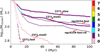 |
Fig. 3 Same as Fig. 2, but for cluster complex “NGC6334” and 2371 M⊙ cluster. |
| In the text | |
|
Fig. 4 Evolution of 3000 M⊙ cluster under different gas-expulsion modes. Snapshots projected on the XY plane (20 pc × 20 pc around the cluster center) at ages 10 Myr, 50 Myr, and 100 Myr are shown here. The size of the black dots reflects the stellar mass (linear scale). Neutron stars and black holes are represented by orange plus signs and red dots, respectively, with the symbol sizes being purely illustrative. The central regions of the star clusters in Figs. 4a and b contain two and three black holes, respectively. In panel b, two of the three black holes are too close to be distinguished on the map. |
| In the text | |
|
Fig. 5 Velocity distribution of stars within cluster complex “NGC6334” and 2371 M⊙ cluster under different gas-expulsion modes at 20 Myr. (a) Probability density function (PDF) of stellar velocities, estimated using the kernel-density-estimation (KDE) method to provide a smooth representation of the distribution; (b) cumulative fraction shows the proportion of stars with velocities below a given value. Here, we do not distinguish between binaries and single stars; instead, we calculated the total velocity of each star (vtot) in the cluster and examined their distribution to roughly characterize the expansion state of the cluster. At 50 Myr, the velocity distributions remain unchanged, indicating that the binary fraction does not significantly affect the statistical results here. |
| In the text | |
|
Fig. 6 Temporal evolution of distance between each pair of black holes. Panels a and b correspond to black-hole pairs in panels a and b of Fig. 4, respectively. |
| In the text | |
Current usage metrics show cumulative count of Article Views (full-text article views including HTML views, PDF and ePub downloads, according to the available data) and Abstracts Views on Vision4Press platform.
Data correspond to usage on the plateform after 2015. The current usage metrics is available 48-96 hours after online publication and is updated daily on week days.
Initial download of the metrics may take a while.