| Issue |
A&A
Volume 704, December 2025
|
|
|---|---|---|
| Article Number | A273 | |
| Number of page(s) | 7 | |
| Section | Interstellar and circumstellar matter | |
| DOI | https://doi.org/10.1051/0004-6361/202554492 | |
| Published online | 17 December 2025 | |
Molecular hydrogen in filaments at high Galactic latitudes
Argelander-Institut für Astronomie, University of Bonn,
Auf dem Hügel 71,
53121
Bonn,
Germany
★ Corresponding author: This email address is being protected from spambots. You need JavaScript enabled to view it.
Received:
12
March
2025
Accepted:
21
November
2025
Abstract
Context. Neutral atomic hydrogen (H I) absorption lines can be used to probe the cold neutral medium (CNM) at high Galactic latitudes. Cold H I with a significant optical depth from the GASKAP-H I survey is found to be located predominantly if not exclusively within filamentary structures that can be identified as caustics with the Hessian operator. Most of these H I filaments (57%) are also observable in the far-infrared (FIR) and trace the orientation of magnetic field lines.
Aims. We considered whether molecular hydrogen (H2) might also be preferentially associated with CNM filaments.
Methods. We analyzed 241 H2 absorption lines against stars and determined whether the lines of sight intersected H I or FIR filaments. Using Far Ultraviolet Spectroscopic Explorer (FUSE) H2 data in the velocity range −50 < vLSR < 50 km s−1, we traced 65 additional H2 lines for filamentary H I and FIR structures in velocity and probed the H2 absorption for coincidences in position and velocity.
Results. For 305 out of 306 positions, the lines of sight with H2 absorption intersect H I filaments. In 120 cases, there is also evidence for a correlation with dusty FIR filaments. All of the 65 available sight lines with known velocities intersect H I filaments. In 64 cases, the H2 velocities are consistent with H I filament velocities. For FIR filaments, an agreement is found for only 13 out of 14 H2 absorption lines.
Conclusions. For the majority of H2 absorption lines, there is evidence that H2 is associated with cold H I filaments. Evidence of an association with FIR filaments is less compelling. Confusion along the line of sight limits the detectability of FIR filaments. For a comparable degree of UV excitation in the disk and lower Galactic halo, the formation rate of H2 appears to be enhanced in H I filaments with increased CNM densities.
Key words: ISM: clouds / dust, extinction / ISM: molecules / ISM: structure
© The Authors 2025
 Open Access article, published by EDP Sciences, under the terms of the Creative Commons Attribution License (https://creativecommons.org/licenses/by/4.0), which permits unrestricted use, distribution, and reproduction in any medium, provided the original work is properly cited.
This article is published in open access under the Subscribe to Open model. This email address is being protected from spambots. You need JavaScript enabled to view it. to support open access publication.
1 Introduction
Neutral atomic hydrogen (H I) gas is one of the most important tracers of the structure and dynamics of the interstellar medium (ISM). Molecular hydrogen (H2) likewise is the simplest and most abundant molecule, and it provides a link to star formation at different scales. We intend to discuss the properties of the cold neutral medium (CNM), in particular, the transition between the atomic and molecular phase in the diffuse atomic medium. This phase is characterized by typical H I excitation temperatures 30 ≲ Tex ≲ 100 K, densities of 10 ≲ nHI ≲ 100 cm−3, and dust temperatures of 15 ≲ Td ≲ 20 K. The H I column densities are below NH = 1021.7 cm−3 and the molecular gas fraction is low, typically fH2 = 2nH2/nH ≲ 0.1 (Snow & McCall 2006; Wakelam et al. 2017).
Detailed H I observations in this temperature regime demand sensitive optical depth measurements, which are only possible against sufficiently strong continuum background sources. Within the past two decades, 372 unique H I lines of sight, distributed throughout the sky, have been observed by various authors with several instruments. A compilation of these 21 cm H I absorption and emission data, called BIGHICAT, are summarized in the Supplemental Table 1 of McClure-Griffiths et al. (2023). Significant absorption is listed at 306 BIGHICAT positions. Yet another 462 positions became available only recently from the Galactic Australian Square Kilometre Array Pathfinder Pilot Phase II Magellanic Cloud H I foreground observations (GASKAP-H I, Nguyen et al. 2024). They cover an area of 250 square degrees of the Milky Way foreground toward the Magellanic Clouds. In total, 2714 positions have been observed, resulting in 691 absorption line detections.
The balance of heating and cooling processes in the ISM results in a multiphase medium. The CNM is in pressure balance with a warm neutral medium (WNM) (Wolfire et al. 2003) that dominates most of the observable H I emission. Within the past decade, the evidence mounted that structures on arcminute scales are shaped in a filamentary way and that H I and far-infrared (FIR) emission agree very well (e.g., Clark et al. 2014; Kalberla et al. 2016). The FIR filaments considered here are always associated with H I. These FIR structures are also associated with cold dust, are stretched out along the magnetic field lines, and have been further investigated by Clark et al. (2019), Peek & Clark (2019), Clark & Hensley (2019), Murray et al. (2020), Kalberla et al. (2020), Kalberla & Haud (2023), and Lei & Clark (2024).
Filaments are defined by their particular topology as caustics that correspond to singularities of gradient maps (e.g., Castrigiano & Hayes 2004 or Arnold et al. 1985). As a standard tool for classifying these structures, Kalberla et al. (2021) (hereafter Paper I) have used the Hessian operator, which is based on partial derivatives of the intensity distribution. Filaments can be described in this way as caustics that are associated with cold CNM, an increased CNM fraction, and an enhanced FIR emissivity, and they are understood as coherent H I fibers with local density enhancements in position-velocity space. Kalberla (2024) (hereafter Paper II) has shown that BIGHICAT H I absorption components are exclusively located in filaments with FIR counterparts. Moreover, Kalberla (2025) (hereafter Paper III) has demonstrated that 57% of the GASKAP-H I absorption components are associated with FIR filaments. All of these 691 CNM clouds with detectable absorption are located in H I filaments. Velocities along H I filaments are observable in projection in the plane of the sky and are affected by turbulent motions with typical dispersions 2.48 < σvturb < 3.9 km s−1. In a similar way, velocities of embedded small-scale structures in optical depth are affected by turbulence. The derived scale-dependent velocity distribution agrees with the first law by Larson (1979).
H2 is the simplest and most abundant molecule in the ISM, and its formation precedes the formation of other molecules (Wakelam et al. 2017). In the face of the finding that the cold H I is predominantly organized in filaments, we consider here the question whether H2 as the most significant molecular component in the CNM at high Galactic latitudes might also be distributed in filaments. In Sect. 2 we analyze the available observations. The conclusions are drawn in Sect. 3, and a summary is given in Sect. 4.
2 Observations and data reduction
2.1 Identifying H I and FIR filaments
Filaments are thin, thread-like structures that can numerically be characterized as caustics or local singularities in the data distribution. In the following, we exclusively use the term filaments for structures that satisfy this mathematical classification. Caustics in two-dimensional intensity distributions are uniquely defined (e.g., Arnold et al. 1985 or Castrigiano & Hayes 2004). The Hessian matrix is used in elementary calculus to determine the properties of singularities (for a detailed discussion, we refer to Paper II, and we only present a brief summary here).
Caustics in the intensity distribution can be identified as critical points with eigenvalues λ− < 0. Hessian eigenvalues and the associated eigenvectors were determined throughout the sky for the HI4PI survey (HI4PI Collaboration 2016) in the velocity range −50 < vLSR < 50 km s−1 and simultaneously for the intensity distribution of Planck data at 857 GHz (Planck Collaboration Int. LVII 2020). To obtain an identical resolution for the two databases, the FIR data were smoothed and converted into an nside = 1024 HEALPix grid.
The filaments in H I and FIR were derived from the eigenvalue distributions1. The velocities vHI along an H I filament are the velocities of the local minima of the H I eigenvalues λ−(v) (for examples, see Fig. A.1 of Paper III). All FIR filaments were checked for coincidences with H I filaments. To fit FIR filaments that are aligned with H I structures, the orientation angles of the Hessian eigenvectors were used. The velocity at which the best alignment between H I and FIR orientation angles is found defines the FIR filament velocity vFIR. A tight agreement between FIR and H I filaments was found in narrow velocity intervals of 1 km s−1 (see Table 1 in Paper I). The correlation degrades significantly for larger velocity intervals with the implication that the H I that is observed in filaments and is associated with the 857 GHz FIR structures has to be cold. Using GASKAP-H I absorption data observed by (Nguyen et al. 2024), Paper III verified that these filaments contain CNM.
The correlation analysis is significantly complicated by the fact that the line of sight may intersect several filaments. For H I these filaments are separated in velocity, and no confusion affects the derived parameters. For the FIR, however, the contributions from different filaments (indicated by H I structures) and other background sources cannot be separated. Only the strongest FIR filaments (with low confusion) can be correlated with H I. Paper I considered fiducial eigenvalues λ− < −1.5 K deg−2 in FIR and λ− < −50 K deg−2 in H I to ensure a good correlation between H I and FIR filaments. For these parameters, the average velocity uncertainties between H I and associated FIR filaments are 2.6 km s−1. This rms scatter is associated with uncertainties in matching the H I and FIR orientation angles. These differences are within 3° to 4° on average (fitting Voigt functions or Gaussians, respectively). The resulting velocity field along the FIR filaments projected onto the plane of the sky is homogeneous, with typical velocity fluctuations of 3.8 km s−1.
Considering the high-latitude sky with |b| > 10° (or |b| > 30°), we found that 30% (18%) of the observed nside=1024 HEALPix positions are covered by FIR filaments and 69% (54%) by H I filaments. Figure 1 shows the covering fractions Fc of filaments within single channels at |b| > 10°. The imbalance between the total number of H I and FIR filaments is obvious: About five times more filaments are counted in H I. Line of sight effects severely limitat the detection of the FIR filaments. A similar degradation is noticeable in H I when the velocity resolution is decreased (Paper I). The curves shown in Fig. 1 are only estimates because they depend on constraints on the eigenvalues. Fig. A.2 in Paper III indicates that releasing the constraint λ− < −50 K deg−2 for H I filaments can lead to a detection rate that is higher by 21% when it is applied to GASKAP-H I absorption components.
The global distribution of H I and FIR filaments at high Galactic latitudes shown in Fig. 1 has a dispersion of 8.1 ± 0.1 km s−1 and 7.9 ± 0.1 km s−1. All of the filaments have narrow line widths. They represent a population of small-scale CNM clumps that cannot be resolved individually in observations. These distributions therefore represent global probability distributions for the velocity of CNM clumps in the local vicinity.
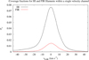 |
Fig. 1 Average filament coverage fractions Fc for FIR and H I filaments within a single velocity channel at Galactic latitudes |b| > 10°. |
2.2 Stellar H2 absorption data, and unknown H2 velocities
Gudennavar et al. (2012) collated absorption line data toward 3008 stars in a unified database of interstellar column densities toward stellar background sources. We used 419 entries for H2 column densities in their Table 2 from the last published values. In total, 416 of these lines of sight intersect H Ifilaments, and 221 of these also intersect FIR filaments. Sources in the Galactic plane might be affected by confusion, and we therefore restricted our analysis in all cases to positions at latitudes |b| > 10°. This sample contains 229 sources, and the lines of sight of 228 sources intersect H I filaments, and 95 lines of sight intersect FIR filaments. We conclude that 99.5% of all detected H2 lines show evidence for a correlation with H I filaments. For 41.7% of the lines of sight, there is also evidence of a correlation with dusty FIR filaments. We conclude that for the sample considered in this section, the detection rate within the filaments increases by 40% with respect to a random distribution. As discussed in Sect. 2.1, the identification of FIR filaments might be limited by confusion. A low identification rate for FIR filaments implies that most of the FIR filaments are weak, with less significant Hessians. In translucent sight lines, Rachford et al. (2002) and Rachford et al. (2009) observed 12 high-latitude lines of sight. All of them intersected H I, and 8 lines of sight (66.7%) intersected FIR filaments, indicating more prominent and better defined FIR filaments in this case.
2.3 FUSE H2 absorption data, and known H2 velocities
The tabulated H2 data we discussed in the previous subsection do not contain any information on the velocity centroids vH2 of the H2 components. We discuss H2 data from the Far Ultraviolet Spectroscopic Explorer (FUSE) with known velocities that can be compared with the velocities ![Mathematical equation: $\[v_{\text {fil}}^{\mathrm{HI}}\]$](/articles/aa/full_html/2025/12/aa54492-25/aa54492-25-eq1.png) and
and ![Mathematical equation: $\[v_{\text {fil}}^{\mathrm{FIR}}\]$](/articles/aa/full_html/2025/12/aa54492-25/aa54492-25-eq2.png) of H I and FIR filaments below.
of H I and FIR filaments below.
A comprehensive database was provided by Wakker (2006), and we used 65 entries that are available within the velocity range −50 < vLSR < 50 km s−12. For each observed line of sight, we first verified whether it was located along a known FIR filament and then derived the velocity difference ![Mathematical equation: $\[\Delta v_{\mathrm{FIR}}=v_{\mathrm{H} 2}-v_{\mathrm{fil}}^{\mathrm{FIR}}\]$](/articles/aa/full_html/2025/12/aa54492-25/aa54492-25-eq3.png) for the associated FIR filament. Next, we considered H I filaments with the velocity difference
for the associated FIR filament. Next, we considered H I filaments with the velocity difference ![Mathematical equation: $\[\Delta v_{\mathrm{HI}}=v_{\mathrm{H} 2}-v_{\text {fil }}^{\mathrm{HI}}\]$](/articles/aa/full_html/2025/12/aa54492-25/aa54492-25-eq4.png) . For multiple H I filaments, the closest match in velocity was selected. As discussed by Paper III, these velocity differences represent local turbulent velocity deviations between the H2, which are probed by absorption within a pencil beam, and the FIR filament with a typical width of 9′. This corresponds to 0.63 pc at an assumed filament distance of 250 pc. For the H I absorption discussed by Paper III, dispersions of
. For multiple H I filaments, the closest match in velocity was selected. As discussed by Paper III, these velocity differences represent local turbulent velocity deviations between the H2, which are probed by absorption within a pencil beam, and the FIR filament with a typical width of 9′. This corresponds to 0.63 pc at an assumed filament distance of 250 pc. For the H I absorption discussed by Paper III, dispersions of ![Mathematical equation: $\[\sigma v_{\text {turb}}^{\mathrm{HI}}=2.48\]$](/articles/aa/full_html/2025/12/aa54492-25/aa54492-25-eq5.png) km s−1 for the whole H I sample, but
km s−1 for the whole H I sample, but ![Mathematical equation: $\[\sigma v_{\text {turb }}^{\text {FIR }}=3.9\]$](/articles/aa/full_html/2025/12/aa54492-25/aa54492-25-eq6.png) km s−1 for FIR filaments was found. We use
km s−1 for FIR filaments was found. We use ![Mathematical equation: $\[\sigma v_{\text {turb}}^{\mathrm{HI}}=2.48\]$](/articles/aa/full_html/2025/12/aa54492-25/aa54492-25-eq7.png) km s−1 below as a reference for comparison.
km s−1 below as a reference for comparison.
We found that all of the 65 low-velocity H2 components from the catalog of Wakker (2006) are associated with H I filaments, but only 14 are associated with FIR filaments. The results are displayed in Fig. 2. At the top, we show a comparison of H2 LSR velocities with the velocities of FIR filaments. The black symbols show a nearly linear relation between H2 and H I velocities, and the deviations have a dispersion of σHI = 4 km s−1. At the bottom of Fig. 2, we show histograms of the velocity deviations vH2 − vfil. We compare these distributions with the reference distribution of σ ~ 2.48 km s−1, as determined by Paper III. The observed deviations ΔvHI (black) are compatible with this reference, except for a few outliers with ![Mathematical equation: $\[\left|v_{\mathrm{H} 2}-v_{\text {fil }}^{\mathrm{HI}}\right| \gtrsim 10\]$](/articles/aa/full_html/2025/12/aa54492-25/aa54492-25-eq8.png) km s−1 (4σ with respect to the reference distribution). The velocity deviations ΔvFIR (red) are barely compatible with the reference distribution.
km s−1 (4σ with respect to the reference distribution). The velocity deviations ΔvFIR (red) are barely compatible with the reference distribution.
An alternative database with 40 FUSE H2 absorption lines was provided by Gillmon et al. (2006). We processed these data in the same way as the data by Wakker (2006) discussed above. Figure 3 displays the results for 40 absorption lines. The plot at the top shows a good linear relation between H2 and H I velocities, in this case, with a dispersion of σHI = 3.6 km s−1. The histogram for vH2 − vfil (bottom) shows a somewhat weird double-peaked structure, but has fewer outliers. The details of the velocity distributions shown in Figs. 2 and 3 might be affected by line blending, or by ambiguities in assigning H I filaments to H2 absorption structures in a few cases. The general characteristics of the velocity distributions remain unaffected, however.
The 40 sight lines used by Gillmon et al. (2006) are in common with Wakker (2006). The discrepancies between Figs. 2 and 3 can be explained by problems in the FUSE wavelength calibration and different approaches to solving the calibration uncertainties. The FUSE velocity resolution at the full width at half maximum (FWHM) depends on the data binning and typically is 20 km s−1 (Wakker 2006, Sect. 4.2). The velocity centroids were estimated by Gillmon et al. (2006, Sect. 2.2) to be uncertain by 5 km s−1 on average. Calibration problems and uncertainties of 2 km s−1 for sight lines with a high signal-to-noise ratio (S/N) and simple absorption-line structure up to 6–8 km s−1 for low S/N data were reported by Wakker (2006, Sect. 2.2)3 (for details, we refer to the extended discussions in that paper). We derived average velocity discrepancies with a dispersion of 5.7 km s−1 from an intercomparison of the two datasets that were used to derive Figs. 2 and 3. Typical 21 cm emission lines in cold H I filaments have dispersions of ~1.3 km s−1 (e.g., Clark et al. 2014 and Kalberla et al. 2016). Filaments, using the Hessian operator, were determined on a velocity grid with a resolution of 1 km s−1 (Paper I).
All of the velocity uncertainties discussed above were compared with observed turbulent velocity fluctuations for the CNM of about σv = 2.48 km s−1 on arcminute scales in the plane of the sky and within a single-dish beam (Paper III). For prominent FIR filaments, the observed dispersion can be up to 3.9 km s−1. According to the first law by Larson (1979), turbulent motions cause scale-dependent velocity fluctuations in the ISM. The velocity dispersion increases with distance l as σv(l) ∝ lq. For supersonic turbulence, the exponent q is expected to be in the range 1/3 ≲ q ≲ 1/2; q = 0.5 applies to the molecular cloud regime (Heyer et al. 2009) and also to the CNM. The relation of line width to size was verified for H I absorption components over distances from 7″ to 10° (Paper III, Fig. 4).
To gain a deeper insight into the properties of the H2 distribution, we plot in Fig. 4 the H2 fraction logfH2 derived by Gillmon et al. (2006) as a function of vH2 − vfil. Figure 5 alternatively shows the relation between H2 column densities and vH2 − vfil derived by Wakker (2006). As noted before by Gillmon et al. (2006), logNH2 ~ 17 appears to separate two populations of H2 absorbers. A similar gap exists in Fig. 4 at logfH2 ~ −3. Adopting turbulent velocity fluctuations with σturb = 2.48 km s−1 as a reference, we considered |vH2 − vfil| ≳ 10 km s−1 as misidentifications and excluded these positions from the discussion. Because of the low number statistics for FIR filaments, we also excluded FIR filaments. With these restrictions, the scatter |vH2 − vfil| increases in Fig. 5 for logNH2 ≲ 17 by a factor of two with respect to logNH2 ≳ 17. The average dispersion is 3.6 km s−1 and in the range 2.48 < σvturb < 3.9 km s−1, observed for H I absorption discussed by Paper III. Turbulence is also observable in the distribution of the metal lines. Comparing H2 velocities with the velocities of metal lines, Wakker (2006) derived from his Table 2 a compatible dispersion of 3.9 km s−1 with peak deviations up to ±9 km s−1. For the wavelength calibration problems discussed by Wakker (2006, Sect. 2.2 and 4.2), it is plausible that the center velocities of sight lines with a low column density have significantly increased uncertainties. These uncertainties also explain the differences in the dispersions that are visible in Figs. 2 and 3. The extended wings in Figs. 2 are caused by sources with low H2 column densities, which explains the high uncertainties in the velocity centroids. In the light of these problems, we conclude that the observed scatter in vH2 − vHI and vH2 − vFIR is significantly affected by observational uncertainties, but is still consistent with the turbulent velocity field shown in Fig. 4 of Paper III.
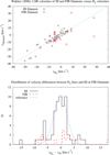 |
Fig. 2 Comparison of velocities from H2 absorption and filaments in H I and FIR. Top: Direct comparison between vH2 and filament velocities vHI (black) or vFIR (red) as defined in Sect. 2.1. Bottom: Histogram of the velocity deviations |
![Mathematical equation: $\[v_{\mathrm{H} 2}-v_{\mathrm{fil}}^{\mathrm{HI}}\]$](/articles/aa/full_html/2025/12/aa54492-25/aa54492-25-eq9.png)
![Mathematical equation: $\[\sigma v_{\text {turb}}^{\mathrm{HI}}=2.48\]$](/articles/aa/full_html/2025/12/aa54492-25/aa54492-25-eq10.png)
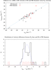 |
Fig. 3 Comparison of velocities from H2 absorption and filaments in H I and FIR. Top: direct comparison between vH2 and filament velocities vHI (black) or vFIR (red) as defined in Sect. 2.1. Bottom: histogram of the velocity deviations |
![Mathematical equation: $\[v_{\mathrm{H} 2}-v_{\mathrm{fil}}^{\mathrm{HI}}\]$](/articles/aa/full_html/2025/12/aa54492-25/aa54492-25-eq11.png)
![Mathematical equation: $\[\sigma v_{\text {turb}}^{\mathrm{HI}}=2.48\]$](/articles/aa/full_html/2025/12/aa54492-25/aa54492-25-eq12.png)
3 Discussion
The ISM is dominated by a multiphase medium (Wolfire et al. 2003) with a diffuse WNM and a clumpy CNM in pressure equilibrium. Large-scale H I surveys such as HI4PI (HI4PI Collaboration 2016) or GALFA-H I (Peek et al. 2018) have led to the picture that a major part of the cold ISM is organized in filamentary structures that are aligned with the magnetic field lines (e.g., Clark et al. 2014; Kalberla et al. 2016). These structures are detectable with the Hessian operator as caustics. Based on this classification, filaments can rigorously be characterized in the FIR with a coherent velocity field and in H I with an extended network of H I fibers at distinct velocities (Paper II). H I and FIR filaments are both exposed to a turbulent external medium, which leads to characteristic velocity fluctuations along and within the filaments.
A detailed analysis of the CNM in filaments became available with the GASKAP-H I absorption line survey, which covers nine adjacent fields of with over 25 square-degrees in the direction to the Magellanic clouds (Nguyen et al. 2024). The analysis of 691 absorption components in 462 lines of sight has led to major improvements in the understanding of the physical properties of the CNM. It was subsequently found that all H I absorption line components are associated with filamentary structures in H I and/or FIR (Paper III), suggesting that a major part of the CNM is located in filaments. The GASKAP-H I components have a mean column density of NHI = 1.81020 cm−2 and a mean spin temperature of Ts = 50 K, and in pressure eqilibrium with the WNM with log(p/k) = 3.58 (Jenkins & Tripp 2011), a mean volume density nHI = 76 cm−3 can be derived. The question arises whether these conditions support a transition from H I to H2. If this is the case, we expect that H2 might also share the filamentary nature of the CNM.
Analyzing published H2 absorption data, we found that 305 out of 306 lines of sight are located along H I filaments in total. A subset of 64 absorption lines has known H2 center velocities. These components, again with a single exception, can also be assigned to H I filaments in velocity4. The observed deviations vH2 − vHI are consistent with the turbulent velocity fluctuations from the GASKAP-H I data (Paper III). Assuming that the H2 formation is supported in presence of CNM with parameters as observed by GASKAP-H I, we conclude that the observable H2 may predominantly be located in cold H I filaments.
This inference is indirect and needs H I absorption data for verification. These observations are missing, except for a single case. Only for the source 3C273 (QSO B1226+0219) can a link between H2, H I, and dust be established. The line of sight to 3C273 intersects an FIR filament with a dust temperature of Td = 17.978 ± 0.013 K (Shull & Panopoulou 2024). Filaments are observed for H I at vHI = −1 km s−1 and for the FIR at vFIR = −2 km s−1 (see Fig. 6).
In addition, an H I filament lies at vHI = 24 km s−1. We discuss this structure first. A corresponding H2 absorption was observed by Gillmon et al. (2006) at vLSR = 26 km s−1 and by Wakker (2006) at vLSR = 28 km s−15. The H I absorption with τ = 0.002 is too weak for us to measure a significant spin temperature, but Heiles & Troland (2003) determined with the Arecibo telescope an upper limit of 87 K for the excitation temperature at this velocity. For a local equilibrium pressure of log(p/k) = 3.58 (Jenkins & Tripp 2011), we estimated the density to be nCNM ≲ 44 cm−3. This is evidence that H2 at the velocity 24 ≲ vLSR ≲ 28 km s−1 is associated with an H I filament at vLSR = 24 km s−1.
Particular cold H I was observed at vLSR = −6.3 km s−1. Heiles & Troland (2003) determined a spin temperature of Ts = 44.4 K, and Murray et al. (2018) reported Ts = 17 K. In pressure equilibrium, the density is 86 ≲ nCNM ≲ 223 cm−3. This component is associated with H I gas at vLSR = −5.5 km s−1 (Heiles & Troland 2003) or vLSR = −5.8 km s−1 (Murray et al. 2018), belonging to the unstable neutral medium (UNM) with a spin temperature of 651 K or 455 K, respectively. As discussed by Heiles & Troland (2003, Sect. 4.5.2), overlapping opacity components cause considerable uncertainties in the Gaussian fit parameters. The H I velocity of vLSR = −6.3 km s−1 is well defined and agrees with the H2 absorption observed at vH2 = −5 km s−1 by (Gillmon et al. 2006), but differs significantly from vH2 = −9 km s−1 derived by Wakker (2006, Sect. 4.2) in presence of considerable uncertainties in the H2 velocity calibration. The observations by Heiles & Troland (2003) indicated CNM column densities of NHI = 4 × 1018 cm−2 with associated column densities of NHI = 46 × 1018 cm−2 for the UNM. Murray et al. (2018) determined for the CNM NHI = 2 × 1018 cm−2, and for the UNM, NHI = 29 × 1018 cm−2. Despite the observational uncertainties, we conclude that the structures observed in FIR, H2 and H I are related. 3C273 is one of the strongest continuum sources, allowing high S/N detections in H I and H2 absorption. The velocity deviations vH2 − vHI are within the uncertainties that are consistent with the turbulent velocity field from GASKAP-H I (Paper III). The filaments are indicated in Fig. 5.
Consistent with previous GASKAP-H I results, our current analysis leads to detection rates close to 100% for absorption lines associated with H I filaments. We compare this with expectations for a random filament distribution. The joint probability P to detect absorption along a filament depends on Fc, the average filament coverage per channel, as shown in Fig. 1, on the filament velocity vfil, and further, on the expected turbulent velocity dispersion σturb along the filament,
![Mathematical equation: $\[P=\int F_c(v) \frac{1}{\sqrt{2 \pi \sigma_{\text {turb }}^2}} \exp ^{-\frac{\left(v-v_{\text {fil }}\right)^2}{2 \sigma_{\text {turb }}^2}} d v.\]$](/articles/aa/full_html/2025/12/aa54492-25/aa54492-25-eq13.png) (1)
(1)
Using ![Mathematical equation: $\[\sigma_{\text {turb}}^{\mathrm{HI}}=2.48\]$](/articles/aa/full_html/2025/12/aa54492-25/aa54492-25-eq14.png) km s−1 and
km s−1 and ![Mathematical equation: $\[\sigma_{\text {turb}}^{\mathrm{FIR}}=3.9\]$](/articles/aa/full_html/2025/12/aa54492-25/aa54492-25-eq15.png) km s−1 we derived for H I filaments an expected probability of PHI = 0.112 ± 0.033 and PFIR = 0.0085 ± 0.0037 for FIR filaments. For reference, we compared these results with GASKAP-H I absorption observations (Nguyen et al. 2024). In this case, we derived probabilities of PHI = 0.126 ± 0.013 for H I and PFIR = 0.0112 ± 0.0014 for the FIR filaments discussed by Paper III. In summary, compared to a random distribution, the observed detection rate for H2 or H I absorption associated with H I filaments is higher by a factor of eight to nine and even higher than 20 for FIR filaments.
km s−1 we derived for H I filaments an expected probability of PHI = 0.112 ± 0.033 and PFIR = 0.0085 ± 0.0037 for FIR filaments. For reference, we compared these results with GASKAP-H I absorption observations (Nguyen et al. 2024). In this case, we derived probabilities of PHI = 0.126 ± 0.013 for H I and PFIR = 0.0112 ± 0.0014 for the FIR filaments discussed by Paper III. In summary, compared to a random distribution, the observed detection rate for H2 or H I absorption associated with H I filaments is higher by a factor of eight to nine and even higher than 20 for FIR filaments.
The derived overdensity suggests that the cold and dense regions that give rise to detectable absorption lines in H2 and H I are located within H I filaments. The detection rate R for FIR filaments, however, is affected by systematical environmental fluctuations. For GASKAP-H I data in the direction of two prominent FIR filaments, a rate of R = 0.57 was found (Paper III). For stellar H2 lines, which are distributed throughout the high-latitude sky, we obtained R = 0.43. This might be representative for the high-latitude sky. For the FUSE absorption observations lines against AGN, we only obtained R = 0.26. A sample in the direction of translucent sight lines yields R = 0.66, however. The margin in R can be explained by selection effects. We considered the two extreme cases. The sample studied by Wakker (2006) is in directions with low extinction (R = 0.26), while translucent sight lines (R = 0.66) contain significant amounts of dust. These regions can provide sufficient protection from interstellar radiation, which would support an increased H2 content. Photodissociation is assumed to be generally the dominant H2 removal mechanism (Wakelam et al. 2017), and less dissociation is expected for translucent sight lines. Dissociation is also minimized for condensed structures with high density. We therefore rejected the ideas that absorption lines and filaments might be caused by an observational accumulation from numerous separate volume elements along the line of sight by a velocity-crowding effect (Yuen et al. 2024).
The case of H2, which might be produced in structures that are much denser than the clouds on average, was considered by Valdivia et al. (2016). These authors performed high-resolution magnetohydrodynamical (MHD) colliding-flow simulations to study the H2 formation of multiphase molecular clouds. As a result of a combination of thermal pressure, ram pressure, and gravity, the clouds produced at the converging point of HI streams were highly inhomogeneous. These authors demonstrated in their Fig. 13 that the derived molecular fractions as function of total hydrogen column density compare well with observations by Gillmon et al. (2006) and Rachford et al. (2002, 2009). Their Fig. B.1 shows that the total shielding coefficient for H2 at column densities logNH2 ≲ 20 is little affected by an absence of shielding by dust. The translucent sight lines observed by Rachford et al. (2002, 2009) have logNH2 ≳ 20; shielding is expected to be strong. Thus, environmental conditions might explain our finding that the detection rate R for H2 absorption in FIR filaments is higher in translucent regions.
The MHD colliding-flow simulations by Valdivia et al. (2016, Figs. 8 and 9) showed that H2 can be formed quickly, within two or three million years for typical volume densities and spin temperatures as observed in the GASKAP-H I sample. Compressible forcing leads to the formation of clumps that are significantly denser than for solenoidal turbulent forcing (Micic et al. 2012). For 3C273, which lies in direction of radio loops I and IV (Panopoulou et al. 2021) at a distance of ~112 pc, there is some evidence that the observed H I distribution might be affected by shocks from supernova events. In comparison to the CNM, ten times more UNM is observed. Most of the cold H I is therefore probably in transition from the WNM to the CNM.
Processes that lead to an H1 to H2 transition for turbulent forcing under various conditions were studied with MHD simulations by Bellomi et al. (2020). In this case, the observed correlation between the H I and H2 column density (Bellomi et al. 2020, Fig. 3) is reproduced well for H2, which is built up in CNM structures between ~3 and ~10 pc. H2 for fractions logfH2 ≲ −3 and column densities logNH2 ≲ 17 are built up from diffuse low-density components along the line of sight, while dense small-scale clumps cause high H2 column densities (Bellomi et al. 2020, Fig. 7). The locations of the 3C273 data within Figs. 4 and 5 are indicated in both cases in the lower parts of the plots. This regime, based on the model by Bellomi et al. (2020), is expected to be occupied by diffuse low-density components (n ≲ 8 cm−3). The observed CNM densities for 3C273 (nCNM ≳ 86 cm−3) exceed the model distribution significantly. Likewise the mean densities from the GASKAP-HI sample (nCNM ~ 76 cm−3) do not fit the model in Fig. 7 of Bellomi et al. (2020). We conclude that a model for turbulent forcing without additional compressible contributions is not supported by H I absorption observations so far.
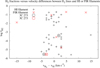 |
Fig. 4 H2 fraction logfH2 derived by Gillmon et al. (2006) vs. observed velocity deviations vH2 − vfil. The filament velocities are vHI (black) or vFIR (red), as defined in Sect. 2.1. |
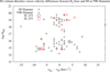 |
Fig. 5 H2 column densities logNH2 derived by Wakker (2006) vs. observed velocity deviations vH2 − vfil. The filament velocities are vHI (black) or vFIR (red), as defined in Sect. 2.1. |
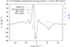 |
Fig. 6 HI4PI brightness temperatures (blue) at the position of 3C 273 and associated eigenvalues λ− (black). H I caustics exist at vLSR = −1 and + 24 km s−1. The FIR caustic is at vLSR = −2 km s−1. The arrows sketch absorption components observed by Murray et al. (2018) and Heiles & Troland (2003) at vLSR = −6.3 and vLSR = 24.2 km s−1. |
4 Summary and conclusions
Recent sensitive H I absorption observations (Nguyen et al. 2024) have shown that the location of CNM in the plane of the sky is predominantly along H I filaments (Paper III), as observed with large single-dish telescopes throughout the sky. A fraction of these filaments can also be traced in the FIR. The turbulent velocity distribution is characteristic for the 3D distribution along the filaments, which is consistent with the first law by Larson (1979). Inspired by these results, we investigated whether the observed H2 distribution is also consistent with the H I results.
We found that most of the known H2 absorption lines are located along H I filaments. Only for a few of these data were velocity centroids determined as well, and H I absorption data are available for only a single source. This is clearly an observational deficit that limitats the credibility of the data analysis. Additional deficits are caused by problems in the wavelength or velocity calibration of the FUSE observations. Wakker (2006) and Gillmon et al. (2006) provided different solutions with an average velocity discrepancy of 5.7 km s−1. These data need to be considered with care. In 64 out of 65 lines of sight are the H2 velocities with derived turbulent velocity fluctuations still consistent with the H I filament velocities discussed by Paper III, however.
High-sensitivity H I absorption lines are available in the direction to 3C273, which is one of the strongest radio sources. These lines confirm the expectation that H2 is correlated with the CNM along filaments in position and velocity. H2 formation is expected to be enhanced in the presence of cold and dense H I (e.g. Valdivia et al. 2016). We are confident that these results can be generalized, and we expect that H2 with increased densities predominantly exists within CNM filaments. Additional H I observations at positions with known H2 absorbers are encouraged.
The formation of H2 in the gas phase is not very relevant to interstellar environments (Vidali 2013; Valdivia et al. 2016). The preference of H2 to accumulate in H I filaments only implies that the CNM in filaments provides perfect conditions to support H2 formation. These conditions are given by cold H I associated with cold dust (Nguyen et al. 2024, Fig. 17) that has settled in H1 filaments. The direct observational evidence for H2 in FIR filaments is affected by sensitivity limitations (see, e.g., Fig. 4 of Kalberla et al. 2016). Only the most prominent FIR filaments are easily observable. Assuming, on the other hand, an increased formation rate for H2 in regions with cold H I at high Galactic latitudes leads to filamentary structures on large scales (Kalberla et al. 2016, Fig. 11), without the need to invoke a sophisticated Hessian analysis (see also Skalidis et al. 2024).
Acknowledgements
I thank the second referee for constructive criticism that helped to improve the paper. HI4PI is based on observations with the 100-m telescope of the MPIfR (Max-Planck-Institut für Radioastronomie) at Effelsberg and Murriyang, the Parkes radio telescope, which is part of the Australia Telescope National Facility (https://ror.org/05qajvd42) which is funded by the Australian Government for operation as a National Facility managed by CSIRO. This research has made use of NASA’s Astrophysics Data System. Some of the results in this paper have been derived using the HEALPix package.
References
- Arnold, V. I., Varchenko, A., & Gusein-Zade, S. M. 1985, Singularities of Differentiable Maps, I: The Classification of Critical Points Caustics and Wave Fronts (Boston: Birkhäuser) [Google Scholar]
- Bellomi, E., Godard, B., Hennebelle, P., et al. 2020, A&A, 643, A36 [NASA ADS] [CrossRef] [EDP Sciences] [Google Scholar]
- Castrigiano, D., & Hayes, S. 2004, Catastrophe Theory, 2nd edn. (CRC Press) [Google Scholar]
- Clark, S. E., & Hensley, B. S. 2019, ApJ, 887, 136 [NASA ADS] [CrossRef] [Google Scholar]
- Clark, S. E., Peek, J. E. G., & Putman, M. E. 2014, ApJ, 789, 82 [NASA ADS] [CrossRef] [Google Scholar]
- Clark, S. E., Peek, J. E. G., & Miville-Deschênes, M.-A. 2019. ApJ, 874 [Google Scholar]
- Gillmon, K., Shull, J. M., Tumlinson, J., et al. 2006, ApJ, 636, 891 [NASA ADS] [CrossRef] [Google Scholar]
- Gudennavar, S. B., Bubbly, S. G., Preethi, K., et al. 2012, ApJS, 199, 8 [NASA ADS] [CrossRef] [Google Scholar]
- Heiles, C., & Troland, T. H. 2003, ApJS, 145, 329 [Google Scholar]
- Heyer, M., Krawczyk, C., Duval, J., et al. 2009, ApJ, 699, 1092 [Google Scholar]
- HI4PI Collaboration (Ben Bekhti, N., et al.) 2016, A&A, 594, A116 [NASA ADS] [CrossRef] [EDP Sciences] [Google Scholar]
- Jenkins, E. B., & Tripp, T. M. 2011, ApJ, 734, 65 [NASA ADS] [CrossRef] [Google Scholar]
- Kalberla, P. M. W. 2024, A&A, 683, A36 [NASA ADS] [CrossRef] [EDP Sciences] [Google Scholar]
- Kalberla, P. M. W. 2025, A&A, 694, L11 [NASA ADS] [CrossRef] [EDP Sciences] [Google Scholar]
- Kalberla, P. M. W., & Haud, U. 2023, A&A, 673, A101 [NASA ADS] [CrossRef] [EDP Sciences] [Google Scholar]
- Kalberla, P. M. W., Kerp, J., Haud, U., et al. 2016, ApJ, 821, 117 [Google Scholar]
- Kalberla, P. M. W., Kerp, J., & Haud, U. 2020, A&A, 639, A26 [EDP Sciences] [Google Scholar]
- Kalberla, P. M. W., Kerp, J., & Haud, U. 2021, A&A, 654, A91 [NASA ADS] [CrossRef] [EDP Sciences] [Google Scholar]
- Larson, R. B. 1979, MNRAS, 186, 479 [NASA ADS] [CrossRef] [Google Scholar]
- Lei, M., & Clark, S. E. 2024, ApJ, 972, 66 [Google Scholar]
- McClure-Griffiths, N. M., Stanimirović, S., & Rybarczyk, D. R. 2023, ARA&A, 61, 19 [NASA ADS] [CrossRef] [Google Scholar]
- Micic, M., Glover, S. C. O., Federrath, C., et al. 2012, MNRAS, 421, 2531 [NASA ADS] [CrossRef] [Google Scholar]
- Murray, C. E., Stanimirović, S., Goss, W. M., et al. 2018, ApJS, 238, 14 [NASA ADS] [CrossRef] [Google Scholar]
- Murray, C. E., Peek, J. E. G., & Kim, C.-G. 2020, ApJ, 899, 15 [CrossRef] [Google Scholar]
- Nguyen, H., McClure-Griffiths, N. M., Dempsey, J., et al. 2024, MNRAS, 534, 3478 [NASA ADS] [CrossRef] [Google Scholar]
- Panopoulou, G. V., Dickinson, C., Readhead, A. C. S., et al. 2021, ApJ, 922, 2, 210 [CrossRef] [Google Scholar]
- Peek, J. E. G., & Clark, S. E. 2019, ApJ, 886, L13 [NASA ADS] [CrossRef] [Google Scholar]
- Peek, J. E. G., Babler, B. L., Zheng, Y., et al. 2018, ApJS, 234, 2 [Google Scholar]
- Planck intermediate results. LVII. 2020, A&A, 643, A42 [NASA ADS] [CrossRef] [EDP Sciences] [Google Scholar]
- Rachford, B. L., Snow, T. P., Tumlinson, J., et al. 2002, ApJ, 577, 221 [Google Scholar]
- Rachford, B. L., Snow, T. P., Destree, J. D., et al. 2009, ApJS, 180, 125 [NASA ADS] [CrossRef] [Google Scholar]
- Shull, J. M., & Panopoulou, G. V. 2024, ApJ, 961, 204 [NASA ADS] [CrossRef] [Google Scholar]
- Skalidis, R., Goldsmith, P. F., Hopkins, P. F., et al. 2024, A&A, 682, A161 [NASA ADS] [CrossRef] [EDP Sciences] [Google Scholar]
- Snow, T. P., & McCall, B. J. 2006, ARA&A, 44, 367 [NASA ADS] [CrossRef] [Google Scholar]
- Valdivia, V., Hennebelle, P., Gérin, M., et al. 2016, A&A, 587, A76 [NASA ADS] [CrossRef] [EDP Sciences] [Google Scholar]
- Vidali, G. 2013, Chem. Rev., 113, 8752 [Google Scholar]
- Wakelam, V., Bron, E., Cazaux, S., et al. 2017, Mol. Astrophys., 9, 1 [Google Scholar]
- Wakker, B. P. 2006, ApJS, 163, 282 [Google Scholar]
- Wolfire, M. G., McKee, C. F., Hollenbach, D., et al. 2003, ApJ, 587 [Google Scholar]
- Yuen, K. H., Ho, K. W., Law, C. Y., et al. 2024, Rev. Mod. Plasma Phys., 8, 21 [Google Scholar]
For downloads of Hessian eigenvalue spectra and filaments, see https://www.astro.uni-bonn.de/hisurvey/AllSky_gauss/index.php
Wakker (2006) presents measurements of H2 column densities toward 73 extragalactic targets but discusses predominantly absorption within high and intermediate velocity clouds.
Gillmon et al. (2006) required S/R > 4, after binning 8 pixels at most.
For seven sources observed by Wakker (2006) no significant H2 lines could be detected. Velocities determined from metal lines were found in four of these cases to be consistent with H I filament velocities, however. For a single source, no caustic was found, and two cases remained without conclusive absorption lines.
In his Table 4 a velocity vLSR = 25 km s−1 is given.
All Figures
|
Fig. 1 Average filament coverage fractions Fc for FIR and H I filaments within a single velocity channel at Galactic latitudes |b| > 10°. |
| In the text | |
|
Fig. 2 Comparison of velocities from H2 absorption and filaments in H I and FIR. Top: Direct comparison between vH2 and filament velocities vHI (black) or vFIR (red) as defined in Sect. 2.1. Bottom: Histogram of the velocity deviations |
| In the text | |
|
Fig. 3 Comparison of velocities from H2 absorption and filaments in H I and FIR. Top: direct comparison between vH2 and filament velocities vHI (black) or vFIR (red) as defined in Sect. 2.1. Bottom: histogram of the velocity deviations |
| In the text | |
|
Fig. 4 H2 fraction logfH2 derived by Gillmon et al. (2006) vs. observed velocity deviations vH2 − vfil. The filament velocities are vHI (black) or vFIR (red), as defined in Sect. 2.1. |
| In the text | |
|
Fig. 5 H2 column densities logNH2 derived by Wakker (2006) vs. observed velocity deviations vH2 − vfil. The filament velocities are vHI (black) or vFIR (red), as defined in Sect. 2.1. |
| In the text | |
|
Fig. 6 HI4PI brightness temperatures (blue) at the position of 3C 273 and associated eigenvalues λ− (black). H I caustics exist at vLSR = −1 and + 24 km s−1. The FIR caustic is at vLSR = −2 km s−1. The arrows sketch absorption components observed by Murray et al. (2018) and Heiles & Troland (2003) at vLSR = −6.3 and vLSR = 24.2 km s−1. |
| In the text | |
Current usage metrics show cumulative count of Article Views (full-text article views including HTML views, PDF and ePub downloads, according to the available data) and Abstracts Views on Vision4Press platform.
Data correspond to usage on the plateform after 2015. The current usage metrics is available 48-96 hours after online publication and is updated daily on week days.
Initial download of the metrics may take a while.