Cesam2k20: A code for a new generation of stellar evolution models

L. Manchon; M. Deal; J. P. C. Marques; Y. Lebreton

doi:10.1051/0004-6361/202554806

Home

All issues

Volume 704 (December 2025)

A&A, 704 (2025) A79

Full HTML

Open Access

Issue		A&A Volume 704, December 2025


Article Number		A79
Number of page(s)		16
Section		Numerical methods and codes
DOI		https://doi.org/10.1051/0004-6361/202554806
Published online		08 December 2025

A&A, 704, A79 (2025)

I. Description of the code

L. Manchon¹^★, M. Deal², J. P. C. Marques³ and Y. Lebreton¹^,4

¹ LIRA, Observatoire de Paris, Université PSL, Sorbonne Université, Université Paris Cité, CY Cergy Paris Université, CNRS, 92190 Meudon, France
² LUPM, Université de Montpellier, CNRS, place Eugène Bataillon, 34095 Montpellier, France
³ Institut d’Astrophysique Spatiale, Université Paris-Saclay, Orsay, France
⁴ Université de Rennes, CNRS, IPR (Institut de Physique de Rennes) – UMR 6251, 35000 Rennes, France

^★ Corresponding author: louis.manchon@obspm.fr

Received: 27 March 2025
Accepted: 21 October 2025

Abstract

We present Cesam2k20, the latest version of the hydrostatic stellar evolution code CESAM originally developed by P. Morel and collaborators. Over the last three decades, it has undergone many improvements and has been extensively tested against other stellar evolution codes before being selected to compute the first-generation grid of stellar models for the PLATO mission. Among all the developments made thus far, Cesam2k20 now implements state-of-the-art models for the transport of chemical elements and angular momentum. It was recently made publicly available with an ecosystem of other codes interfaced with it: 1D and 2D oscillation codes ADIPLS and ACOR, optimisation program OSM, and Python utility package pycesam. This paper recalls the numerical peculiarities of Cesam2k20, namely, the use of a collocation method where the structure variables are decomposed as piecewise polynomials projected on a B-spline basis. Here, we review the options available for modelling the different physical processes. In particular, we illustrate the improvements made in the transport of chemical elements and angular momentum with a series of standard and non-standard solar models.

Key words: methods: numerical / Sun: evolution / Sun: interior / stars: evolution / stars: interiors

© The Authors 2025

Open Access article, published by EDP Sciences, under the terms of the Creative Commons Attribution License (https://creativecommons.org/licenses/by/4.0), which permits unrestricted use, distribution, and reproduction in any medium, provided the original work is properly cited.

This article is published in open access under the Subscribe to Open model. Subscribe to A&A to support open access publication.

1 Introduction

Cesam2k20 is a hydrostatic stellar evolution code that comprises the latest version of the Code d’Évolution Stellaire, Adaptatif et Modulaire (CESAM) stellar evolution code originally developed by Pierre Morel and collaborators. This code was first used to produce standard solar models (Berthomieu et al. 1993), with the numerical details presented in Morel (1997, hereafter M97). CESAM was originally written in FORTRAN 77 for its first four versions and later translated into Fortran 90 for the fifth. In the early 2000s, CESAM was renamed CESAM2k. Morel & Lebreton (2008, hereafter ML08) published a full description of this new version as part of the scientific preparation for the Convection Rotation and Transits mission (CoRoT; Baglin et al. 2006).

The availability of precise asteroseismic data on the stellar interior and the first measurements of internal stellar rotation have motivated sizable efforts to test models of angular momentum transport processes. Such models were implemented in CESAM2k, then renamed CESTAM (where T stands for Transport). Using this code, Marques et al. (2013, hereafter M13) and Goupil et al. (2013a) showed that our understanding of angular momentum transport is far from complete (see Goupil et al. 2013b; Aerts et al. 2019, for a review). A lot of work has also been put into improving the user-friendliness of the code, especially with respect to the automated installation process and new Python (graphical) interface.

The next developments, results of intense collaborative efforts, have been important in the following years. They are now gathered in a new version of the CESAM code for the 2020 decade: Cesam2k20¹. The repository² hosting the public versions will be regularly updated with new versions of Cesam2k20.

This state-of-the-art version has benefited from successive validations and comparisons against other stellar evolution codes. The first validation dates back to the year that followed the publication of the seminal paper with a comparison by Turck-Chièze et al. (1998) of two versions of CESAM with earlier versions or predecessors of ASTEC (Christensen-Dalsgaard 1982, 2008b), GARSTEC (Schlattl et al. 1997; Weiss & Schlattl 2008), CLES (Scuflaire et al. 2008), and the Montreal code (Turcotte et al. 1998; Richer et al. 2000). Over the next few years, it was tested on Hyades binaries (Lastennet et al. 1999), the Hyades cluster (de Bruijne et al. 2001), and red stragglers (Fernandes & Santos 2004), as well as against the Geneva (Eggenberger et al. 2008) and Padova/PARSEC (Bressan et al. 1993, 2012) codes. Prior to the launch of the CoRoT mission, the Evolution and Seismic Tools Activity (ESTA) model comparison project (Lebreton et al. 2008b,a; Montalbán et al. 2008; Lebreton & Michel 2008; Marconi et al. 2008; Goupil 2008), extensively tested almost all the stellar evolution codes existing at that time (for a description of the codes included in the ESTA comparison, see Monteiro 2009). Similar comparisons were performed for higher mass stars (Weiss et al. 2007) and later for the special case of red giant modelling (Silva Aguirre et al. 2020; Christensen-Dalsgaard et al. 2020). The code has been part of many stellar model comparisons in the context the CoRoT mission with CoRoT targets (Castro et al. 2021) against the TGEC code (Hui-Bon-Hoa 2008) and of those the Kepler mission (Silva Aguirre et al. 2013; Reese et al. 2016; Silva Aguirre et al. 2017). More recently, the treatment of atomic diffusion (Campilho et al. 2022) and of the overshoot (Noll & Deheuvels 2023) have been compared with MESA (Paxton et al. 2013).

This code or previous versions have been used to model a wide variety of stars. Of course, starting with the Sun (Berthomieu et al. 1993; Brun et al. 1998, 1999; Samadi et al. 2001; Couvidat et al. 2003; Mecheri et al. 2004) and including solar-like oscillators and Sun-like stars have been primary targets of Cesam2k20 users, including Piau & Turck-Chièze (2002); Ballot et al. (2004); Deheuvels et al. (2010a,b); Metcalfe et al. (2010). However, it has also been used for modelling magnetic stars (Cunha 2006; Alecian et al. 2007a,b, 2009; Villebrun et al. 2019; Alecian & Lebreton 2020), binary stars ι Pegasi A&B (Morel et al. 2000a), α Centauri A & B (Morel et al. 2000b; Thévenin et al. 2002; Kervella et al. 2003), 85 Peg (Fernandes et al. 2002), ζ Her A & B (Lebreton et al. 1993; Morel et al. 2001), EK Cephei A & B (Marques et al. 2004), 61 Cyg A & B (Kervella et al. 2008), and samples of nearby binaries or Gaia and Kepler targets (Fernandes et al. 1998; Appourchaux et al. 2015; Kiefer et al. 2016, 2018; Halbwachs et al. 2020), as well as ensembles of stars or cluster members (Fernandes et al. 1996; Cayrel de Strobel et al. 1999; Perryman et al. 1998; Lebreton et al. 1999; Cayrel et al. 2000; Lebreton et al. 2001; Torres et al. 2011) and various classes of pulsators such as solar-like pulsators; these include exoplanet hosts, pre-main sequence stars, subgiants, and red giants (Suran et al. 2001; Lebreton & Goupil 2012; Baudin et al. 2012; Lebreton & Goupil 2014; Crida et al. 2018; Ligi et al. 2019; Huber et al. 2019; Chaplin et al. 2020), λ Bootis stars (Paunzen 1998), δ Scuti stars (Hernandez et al. 1998; Michel et al. 1999; Samadi et al. 2002; Suárez et al. 2002; Amado et al. 2004; Chapellier et al. 2004; Suárez et al. 2005a; Poretti et al. 2005; Fox Machado et al. 2006; Suárez et al. 2006; Casas et al. 2006; Suárez et al. 2007; García Hernández et al. 2009; Poretti et al. 2009), γ Doradus stars (Moya et al. 2005; Suárez et al. 2005b; Ouazzani et al. 2019), blue supergiants (Godart et al. 2009; Lebreton et al. 2009), and Cepheids (Cordier et al. 2002, 2003; Morel et al. 2010). Finally, Cesam2k20 models have supported theoretical works, improving our understanding of asteroseismology and deriving seismic diagnostics (Dintrans & Rieutord 2000; Mazumdar & Antia 2001; Samadi et al. 2001, 2003, 2006; Belkacem et al. 2008, 2009, 2015b,a; Deheuvels et al. 2016; Houdayer et al. 2021) to exploring dark matter models (Lopes et al. 2002; Lopes & Silk 2003; Lopes et al. 2011; Casanellas & Lopes 2011; Casanellas et al. 2015). At the moment, Cesam2k20 can compute stellar models for mass below 20 M_⊙ from the PMS to He-burning; however, low-mass star models cannot pass the He flash. For models to pass the flash, the evolution must be stopped during the red giant branch (RGB) above the red giant bump.

This paper is aimed at presenting the new options available in Cesam2k20 (rather than performing validation, tests, or comparisons). Such developments can be found in the above references. Section 2 provides a concise description of Cesam2k20, as the numerics are already detailed in depth in M97 and ML08. Newly available equations of state (EoS), opacity and nuclear reaction tables are summarized in Sect. 3. Developments in the treatment of convection, evolution of chemicals and of angular momentum, and the restitution of the atmosphere are detailed in Sect. 4, Sect. 5, and Sects. 6 and 7, respectively. As Cesam2k20 is moving forward to be able to compute advanced evolutionary phases, Sect. 8 describes the new mass loss prescriptions implemented. Finally, we illustrate what Cesam2k20 is capable of with standard and non-standard solar models in Sect 9.

2 Cesam2k20’s numerics in brief

Most stellar evolution codes rely on finite element schemes to solve the stellar structure equations and the transport of chemicals. With these schemes, the star is divided into layers and k-th order derivatives are approximated using the values of each quantity at the faces of the nearest layers. Those methods are fast, well tested and easy to implement. However, they provide solutions only at the faces of each layer and not between them. Furthermore, during stellar evolution, the mesh frequently needs to be adapted to resolve regions with strong gradients, and it can be useful to adopt different meshes for solving different systems of equations (i.e. a mesh dedicated to structure equations, another one for the transport of chemicals, etc.). The re-meshing is hindered by the fact that the solutions are only known at a few discrete points.

Cesam2k20 follows quite a peculiar path. Solutions are represented by a linear combination of B-Splines (Schumaker 2007). The B-Splines form an orthogonal basis of piecewise continuous polynomials. The representation of the solution to an equation as a linear combination of B-Splines provides an (approximate) knowledge of this quantity everywhere, by only knowing the exact solution at particular points, known as collocation points. Another advantage is that a different mesh for different systems of equations can be used. For instance, the masses at which the structure equations are solved are not the same as the ones that the equations for the transport of chemicals are solved for. This could also be the case for the transport of angular momentum.

2.1 Grid point allocation

Each spherical shell in the model is labelled with its radius, r_i, and the mass, m_i, enclosed in it. We need to increase the resolution where the gradients of the significant quantities are the strongest. Therefore, the layers should be located in a way that minimizes these gradients or at least that keeps them below a certain threshold. To that end, we introduced a quantity, Q, which serves as the spacing function. This quantity is defined so that, at a given time step, the variation of Q between two consecutive layers of mass, m_i and m_i+1, dis constant, expressed as $Q (m_{i + 1}, t) - Q (m_{i}) = {\frac{d Q}{d q} |}_{t} \equiv ψ (t) = c s t,$ $\[Q\left(m_{i+1}, t\right)-Q\left(m_i\right)=\left.\frac{\mathrm{d} Q}{\mathrm{~d} q}\right|_t \equiv \psi(t)=\mathrm{cst},\]$ (1)

and with ${\frac{d^{2} Q}{d q^{2}} |}_{t} = 0,$ $\[\left.\frac{\mathrm{d}^2 Q}{\mathrm{~d} q^2}\right|_t=0,\]$ (2)

where q is called the index function and takes integer values at each layer, from 1 to n, with n the total number of layers. The function ψ can be written as a function of the mass, ${\frac{d Q}{d q} |}_{t} = {{\frac{d Q}{d m} |}_{t} \frac{d m}{d q} |}_{t} = {θ (t) \frac{d m}{d q} |}_{t} = ψ (t),$ $\[\left.\frac{\mathrm{d} Q}{\mathrm{~d} q}\right|_t=\left.\left.\frac{\mathrm{d} Q}{\mathrm{~d} m}\right|_t \frac{\mathrm{~d} m}{\mathrm{~d} q}\right|_t=\left.\theta(t) \frac{\mathrm{d} m}{\mathrm{~d} q}\right|_t=\psi(t),\]$ (3)

where θ(t) has been identified as dQ/dm|_t. We end up with two more differential equations, which are to be added to the four structure equations, $\frac{d m}{d q} = \frac{ψ}{θ} and \frac{d ψ}{d q} = 0.$ $\[\frac{\mathrm{d} m}{\mathrm{~d} q}=\frac{\psi}{\theta} \text { and } \frac{\mathrm{d} \psi}{\mathrm{~d} q}=0.\]$ (4)

Equations (4) are complemented by boundary conditions: at q = 1, m = 0 and at q = n, m = M_⋆.

We still need a definition for the spacing function Q, that must be a class 𝒞² function, strictly increasing. A simple choice is $Q (m, t) = \frac{p}{Δ p} + \frac{T}{Δ T} + \frac{L}{Δ L} + \frac{r}{Δ r} + \frac{m}{Δ m},$ $\[Q(m, t)=\frac{p}{\Delta p}+\frac{T}{\Delta T}+\frac{L}{\Delta L}+\frac{r}{\Delta r}+\frac{m}{\Delta m},\]$ (5)

where p is the pressure, T the temperature, and L the luminosity, while the terms Δf represent the repartition factors and are aimed at weighting the importance of each quantity. With this definition, Q(m_i+1, t) − Q(m_k) behaves as the sum of the normalized gradients of each independent variable. Each weight Δf can be chosen when running a Cesam2k20 model. However, years of use of Cesam2k20 and preceding version have shown that (1/Δp; 1/ΔT; 1/ΔL; 1/Δr; 1/Δm) = (−1, −1, 0, 0, 15) is a very good choice, at least before He burning phases.

2.2 Dimensionless structure equations

Cesam2k20 assumes hydrostatic equilibrium and solves six differential equations associated with six independent variables r, p, T, L, m, and ψ. The equations for r, p, T, L are the usual structure expressions (and they can be found e.g. in M97, without rotation), while the expressions for ψ and θ are given in Eq. (4). To improve floating-point precision, Cesam2k20 actually solves equation for dimensionless variables: ξ = ln p, η = ln T, λ = (L/L_⊙)^a, ζ = (r/R_⊙)², ν = (m/M_⊙)^2/3, and ψ, which is already dimensionless. The power, a, on the luminosity is either 2/3 or 1. In the past, a = 2/3 was used to avoid derivability issues near the centre, but it is now possible to use a = 1. In terms of these dimensionless variables, the structure equation system is expressed as ${\begin{cases} \frac{\partial ξ}{\partial q} = \frac{- 3 G}{8 π} {(\frac{M_{⊙}}{R_{⊙}^{2}})}^{2} {(\frac{v}{ζ})}^{2} \exp (- ξ) \frac{ψ}{θ}, \\ \frac{\partial η}{\partial q} = \frac{\partial ξ}{\partial q} \nabla, \\ \frac{\partial ζ}{\partial q} = \frac{3}{4 π} \frac{M_{⊙}}{R_{⊙}^{3}} {(\frac{v}{ζ})}^{1 / 2} \frac{1}{ρ} \frac{ψ}{θ}, \\ \frac{\partial λ}{\partial q} = \frac{M_{⊙} v^{1 / 2}}{L_{⊙} λ^{1 / 2}} Λ \frac{ψ}{θ}, with a = 1, \\ \frac{\partial λ}{\partial q} = \frac{3}{2} \frac{M_{⊙} v^{1 / 2}}{L_{⊙}} Λ \frac{ψ}{θ}, with a = \frac{2}{3}, \\ \frac{\partial v}{\partial q} = \frac{ψ}{θ}, \\ \frac{\partial ψ}{\partial q} = 0, \end{cases}$ $\[\left\{\begin{array}{l}\frac{\partial \xi}{\partial q}=\frac{-3 \mathcal{G}}{8 \pi}\left(\frac{M_{\odot}}{R_{\odot}^2}\right)^2\left(\frac{v}{\zeta}\right)^2 \exp (-\xi) \frac{\psi}{\theta}, \\\frac{\partial \eta}{\partial q}=\frac{\partial \xi}{\partial q} \nabla, \\\frac{\partial \zeta}{\partial q}=\frac{3}{4 \pi} \frac{M_{\odot}}{R_{\odot}^3}\left(\frac{v}{\zeta}\right)^{1 / 2} \frac{1}{\rho} \frac{\psi}{\theta}, \\\frac{\partial \lambda}{\partial q}=\frac{M_{\odot} v^{1 / 2}}{L_{\odot} \lambda^{1 / 2}} \Lambda \frac{\psi}{\theta}, \text { with } a=1, \\\frac{\partial \lambda}{\partial q}=\frac{3}{2} \frac{M_{\odot} v^{1 / 2}}{L_{\odot}} \Lambda \frac{\psi}{\theta}, \text { with } a=\frac{2}{3}, \\\frac{\partial v}{\partial q}=\frac{\psi}{\theta}, \\\frac{\partial \psi}{\partial q}=0,\end{array}\right.\]$ (6)

where 𝒢 is the gravitational constant, ∇ ≡ d ln T/d ln p is the temperature gradient, ρ is the density, and M_⊙, R_⊙, and L_⊙ are the solar mass, radius, and luminosity, respectively.

2.3 Collocation method

Let us rewrite the above system of first order ordinary differential equations in a more compact way. By denoting y = (y₁, y₂, y₃, y₄, y₅, y₆) = (ξ, η, ζ, λ, ν, ψ) the unknowns, the system in Eq. (6) may be written as $E (q; y, y^{'}) = \frac{d y}{d q} - g (q, y) = 0 with q \in [q_{1}, q_{n}],$ $\[\mathbf{E}\left(q ; \mathbf{y}, \mathbf{y}^{\prime}\right)=\frac{\mathrm{d} \mathbf{y}}{\mathrm{~d} q}-\mathbf{g}(q, \mathbf{y})=\mathbf{0} \text { with } q \in\left[q_1, q_n\right],\]$ (7)

with g a suitable vector of functions representing the differential system.

The system in Eq. (6), while keeping only a = 1 for simplicity, is then ${\begin{cases} E_{1} = 0 = \frac{\partial y_{1}}{\partial q} - \frac{- 3 G}{8 π} {(\frac{M_{⊙}}{R_{⊙}^{2}})}^{2} {(\frac{y_{5}}{y_{3}})}^{2} \exp (- y_{1}) \frac{y_{6}}{θ}, \\ E_{2} = 0 = \frac{\partial y_{2}}{\partial q} - \frac{\partial y_{1}}{\partial q} \nabla, \\ E_{3} = 0 = \frac{\partial y_{3}}{\partial q} - \frac{3}{4 π} \frac{M_{⊙}}{R_{⊙}^{3}} {(\frac{y_{5}}{y_{3}})}^{1 / 2} \frac{1}{ρ} \frac{y_{6}}{θ}, \\ E_{4} = 0 = \frac{\partial y_{4}}{\partial q} - \frac{M_{⊙} y_{5}^{1 / 2}}{L_{⊙} y_{4}^{1 / 2}} Λ \frac{y_{6}}{θ}, \\ E_{5} = 0 = \frac{\partial y_{5}}{\partial q} - \frac{y_{6}}{θ}, \\ E_{6} = 0 = \frac{\partial y_{6}}{\partial q} . \end{cases}$ $\[\left\{\begin{array}{l}E_1=0=\frac{\partial y_1}{\partial q}-\frac{-3 \mathcal{G}}{8 \pi}\left(\frac{M_{\odot}}{R_{\odot}^2}\right)^2\left(\frac{y_5}{y_3}\right)^2 \exp \left(-y_1\right) \frac{y_6}{\theta}, \\E_2=0=\frac{\partial y_2}{\partial q}-\frac{\partial y_1}{\partial q} \nabla, \\E_3=0=\frac{\partial y_3}{\partial q}-\frac{3}{4 \pi} \frac{M_{\odot}}{R_{\odot}^3}\left(\frac{y_5}{y_3}\right)^{1 / 2} \frac{1}{\rho} \frac{y_6}{\theta}, \\E_4=0=\frac{\partial y_4}{\partial q}-\frac{M_{\odot} y_5^{1 / 2}}{L_{\odot} y_4^{1 / 2}} \Lambda \frac{y_6}{\theta}, \\E_5=0=\frac{\partial y_5}{\partial q}-\frac{y_6}{\theta}, \\E_6=0=\frac{\partial y_6}{\partial q}.\end{array}\right.\]$ (8)

This system is also supplemented with a set of bottom and top boundary conditions, E^b (q₁, y) and E^t(q_n, y). The solution is the set of functions y(q) that makes E_k(q) = 0, ∀k ∈ ⟦1; 6⟧.

This system is solved using a pseudo-spectral method called the collocation method (e.g. De Boor 2001). Unknown functions ${y_{i} (q)}_{i = 1}^{6}$ $\[\left\{y_{i}(q)\right\}_{i=1}^{6}\]$ will be decomposed as a linear combination of B-Splines. We let ${q_{i}}_{i = 0}^{n}$ $\[\left\{q_{i}\right\}_{i=0}^{n}\]$ be a set of points that verify the condition a = q₀ < q₁ . . . < q_n = b, with a and b as the limits of the interval in which Eq. (7) is to be solved. We denote ${N_{j}^{m}}_{j = 1}^{M}$ $\[\{N_{j}^{m}\}_{j=1}^{M}\]$ the basis of B-Splines of the vector space of dimension M of all the piecewise polynomials (of the order³ m) that match at ${q_{i}}_{i = 1}^{n - 1}$ $\[\left\{q_{i}\right\}_{i=1}^{n-1}\]$ . Any unknown y_k of Eq. (7) can be decomposed as $y_{k} (q) = \sum_{j = 1}^{M} y_{k j} N_{j}^{m} (q),$ $\[y_k(q)=\sum_{j=1}^M y_{k j} N_j^m(q),\]$ (9)

and $y_{k}^{'} (q) = \frac{d y_{k}}{d q} = \sum_{j = 1}^{M} y_{k j} \frac{d N_{j}^{m}}{d q} .$ $\[y_k^{\prime}(q)=\frac{\mathrm{d} y_k}{\mathrm{~d} q}=\sum_{j=1}^M y_{k j} \frac{\mathrm{~d} N_j^m}{\mathrm{~d} q}.\]$ (10)

Finally, we define 𝒦 = ⟦1; 6⟧ and ℬ ⊆ 𝒦 (resp. 𝒯 ⊆ 𝒦), which is the set of indices of the unknowns for which a bottom (resp. top) boundary condition is provided. We end up with a set of equations taking the following form:

At the bottom: $E_{k}^{b}$ $\[E_{k}^{\mathrm{b}}\]$ , with k ∈ ℬ is $E_{k}^{b} (\sum_{j = 1}^{M} y_{1, j} N_{j}^{m} (q_{1}); \dots; \sum_{j = 1}^{M} y_{6, j} N_{j}^{m} (q_{1})) = 0 .$ $\[E_k^{\mathrm{b}}\left(\sum_{j=1}^M y_{1, j} N_j^m\left(q_1\right) ; \ldots ; \sum_{j=1}^M y_{6, j} N_j^m\left(q_1\right)\right)=0.\]$ (11)
At the top: $E_{k}^{t}$ $\[E_{k}^{\mathrm{t}}\]$ , with k ∈ 𝒯 is $E_{k}^{t} (\sum_{j = 1}^{M} y_{1, j} N_{j}^{m} (q_{n}); \dots; \sum_{j = 1}^{M} y_{6, j} N_{j}^{m} (q_{n})) = 0 .$ $\[E_k^{\mathrm{t}}\left(\sum_{j=1}^M y_{1, j} N_j^m\left(q_n\right) ; \ldots ; \sum_{j=1}^M y_{6, j} N_j^m\left(q_n\right)\right)=0.\]$ (12)
Elsewhere (q ∈ [q₁; q_n]), for k ∈ 𝒦, $\begin{aligned} E_{k} (q; \sum_{j = 1}^{M} y_{1, j} N_{j}^{m}; \dots; \sum_{j = 1}^{M} y_{6, j} N_{j}^{m}; \\ \sum_{j = 1}^{M} y_{1, j} \frac{d N_{j}^{m}}{d q}; \dots; \sum_{j = 1}^{M} y_{6, j} \frac{d N_{j}^{m}}{d q}) = 0 . \end{aligned}$ $\[\begin{aligned}& E_k\left(q ; \sum_{j=1}^M y_{1, j} N_j^m ; \ldots ; \sum_{j=1}^M y_{6, j} N_j^m ;\right. \\& \left.\quad \sum_{j=1}^M y_{1, j} \frac{\mathrm{~d} N_j^m}{\mathrm{~d} q} ; \ldots ; \sum_{j=1}^M y_{6, j} \frac{\mathrm{~d} N_j^m}{\mathrm{~d} q}\right)=0.\end{aligned}\]$ (13)

The coefficients y_k,j become the unknowns of the system.

On M − 1 collocation points c_k ∈]q₁, q_n[, chosen using Gauss-Legendre quadrature (see De Boor 2001, for details), the coefficients y_i,j are found using an iterative method: the Newton-Raphson method. At first, y_k,j are initialized with the solution found at the previous time step. Then, at a given iteration p ≥ 0, it is estimated by

At the bottom: ∀i ∈ ℬ, $\begin{matrix} E_{i}^{b} (\sum_{j = 1}^{M} y_{1, j}^{p} N_{j}^{m} (q_{1}); \dots; \sum_{j = 1}^{M} y_{n_{e}, j}^{p} N_{j}^{m} (q_{1})) \\ = \sum_{l = 1}^{n_{e}} \sum_{j = 1}^{M} \frac{\partial E_{i}^{b}}{\partial y_{l}} N_{j}^{m} (q_{1}) d y_{l j}^{p} . \end{matrix}$ $\[\begin{gathered}E_i^{\mathrm{b}}\left(\sum_{j=1}^M y_{1, j}^p N_j^m\left(q_1\right) ; \ldots ; \sum_{j=1}^M y_{n_{\mathrm{e}}, j}^p N_j^m\left(q_1\right)\right) \\=\sum_{l=1}^{n_{\mathrm{e}}} \sum_{j=1}^M \frac{\partial E_i^{\mathrm{b}}}{\partial y_l} N_j^m\left(q_1\right) \mathrm{d} y_{l j}^p.\end{gathered}\]$ (14)
At the top: ∀i ∈ 𝒯, we have $\begin{matrix} E_{i}^{t} (\sum_{j = 1}^{M} y_{1, j}^{p} N_{j}^{m} (q_{n}); \dots; \sum_{j = 1}^{M} y_{n_{e}, j}^{p} N_{j}^{m} (q_{n})) \\ = \sum_{l = 1}^{n_{e}} \sum_{j = 1}^{M} \frac{\partial E_{i}^{t}}{\partial y_{l}} N_{j}^{m} (q_{n}) d y_{l j}^{p} . \end{matrix}$ $\[\begin{gathered}E_i^{\mathrm{t}}\left(\sum_{j=1}^M y_{1, j}^p N_j^m\left(q_n\right) ; \ldots ; \sum_{j=1}^M y_{n_{\mathrm{e}}, j}^p N_j^m\left(q_n\right)\right) \\=\sum_{l=1}^{n_{\mathrm{e}}} \sum_{j=1}^M \frac{\partial E_i^{\mathrm{t}}}{\partial y_l} N_j^m\left(q_n\right) \mathrm{d} y_{l j}^p.\end{gathered}\]$ (15)
Elsewhere, ∀j ∈ 𝒦, ∀k ∈ ⟦1; M − 1⟧, we have $\begin{aligned} E_{i} (c_{k}; \sum_{j = 1}^{M} y_{1, j}^{p} N_{j}^{m} (c_{k}); \dots; \sum_{j = 1}^{M} y_{n_{e}, j}^{p} N_{j}^{m} (c_{k}); \\ \sum_{j = 1}^{M} y_{1, j}^{p} \frac{d N_{j}^{m}}{d q} (c_{k}); \dots; \sum_{j = 1}^{M} y_{n_{e}, j}^{p} \frac{d N_{j}^{m}}{d q} (c_{k})) \\ = & \sum_{l = 1}^{n_{e}} \sum_{j = 1}^{M} (\frac{\partial E_{i}}{\partial y_{l}} N_{j}^{m} (c_{k}) + \frac{\partial E_{i}}{\partial y_{l}^{'}} \frac{d N_{j}^{m}}{d q} (c_{k})) d y_{l j}^{p} . \end{aligned}$ $\[\begin{aligned}& E_i\left(c_k ; \sum_{j=1}^M y_{1, j}^p N_j^m\left(c_k\right) ; \ldots ; \sum_{j=1}^M y_{n_{\mathrm{e}}, j}^p N_j^m\left(c_k\right)\right.; \\& \left.\sum_{j=1}^M y_{1, j}^p \frac{\mathrm{~d} N_j^m}{\mathrm{~d} q}\left(c_k\right) ; \ldots ; \sum_{j=1}^M y_{n_{\mathrm{e}}, j}^p \frac{\mathrm{~d} N_j^m}{\mathrm{~d} q}\left(c_k\right)\right) \\= & \sum_{l=1}^{n_{\mathrm{e}}} \sum_{j=1}^M\left(\frac{\partial E_i}{\partial y_l} N_j^m\left(c_k\right)+\frac{\partial E_i}{\partial y_l^{\prime}} \frac{\mathrm{d} N_j^m}{\mathrm{~d} q}\left(c_k\right)\right) \mathrm{d} y_{l j}^p.\end{aligned}\]$ (16)

The quantities $d y_{l j}^{p}$ $\[\mathrm{d} y_{l j}^{p}\]$ are small corrections to the coefficients $y_{l j}^{p}$ $\[y_{l j}^{p}\]$ and are the unknowns of the Newton-Raphson scheme. With the value of $d y_{l j}^{p}$ $\[\mathrm{d} y_{l j}^{p}\]$ , we can determine the value of y_lj at next iteration: $y_{l j}^{p + 1} = y_{l j}^{p} - d y_{l j}^{p}; \forall l \in ⟦ 1; n_{e} ⟧, \forall j \in ⟦ 1; M ⟧ .$ $\[y_{l j}^{p+1}=y_{l j}^p-\mathrm{d} y_{l j}^p ; \quad \forall l \in \llbracket 1 ; n_{\mathrm{e}} \rrbracket, \forall j \in \llbracket 1 ; M \rrbracket.\]$ (17)

The collocation method offers the advantage of superconvergence. Indeed, instead of reaching a precision of order m (m is the order of the B-Splines), the collocation method, by choosing the point in a judicious way, reaches a precision of the order of 2m.

2.4 General flowchart of Cesam2k20

The general path followed by Cesam2k20 to compute the evolution during one time step is summarised in Fig. 1. At a given time step t + Δt, Cesam2k20 starts by evaluating the mass lost or gained according to the chosen prescription (see Sect. 8 for details). Then, based on the structure determined at the previous time step, the new location of the radiative-convective zone (RZ-CZ) transitions is determined, following Schwarzschild’s or Ledoux’s criterion, using the method of Gabriel et al. (2014) (see. Sect. 4 for more details). When we know the precise localisation of RZ and CZ, Cesam2k20 can solve (when needed) equations of the transport of angular momentum (see Sect. 6 for details). If this step is not a success, the time step is divided by 2 and the process is restarted from the beginning. Otherwise, equations for the transport of chemicals are solved. This includes chemical elements created or depleted by nuclear reactions and diffused by microscopic, turbulent, and radiative diffusion (see Sect. 5 for details). Again, depending on the convergence of these operations, the process continues or it is restarted with Δt/2. Finally, the structure equations are solved using the collocation method described above. Afterwards, in addition to some convergence criteria, we also checked that other criteria were met, depending on the precision needed.

The numerical precision can be finely adjusted in Cesam2k20. In addition to parameters that control B-spline orders, number of layers, repartition factors (see Eq. (5)), and other numerical aspects, the user can also choose to limit between each time step, the variation of core temperature or density, the variation of T_eff, log g, and other parameters. This approach can be used to obtain very detailed stellar evolutionary tracks. All these parameters have a default value and a predefined set of values can be selected to achieve super precision, solar accuracy, etc. There exists also pre-defined precision for the CoRoT mission, and for the PLATO grid, as Cesam2k20 was selected to compute the first generation of PLATO’s grid of stellar models.

2.5 Python interface

To facilitate the use of Cesam2k20, we developed a Python utility package over the years. This package is divided into two main parts. The first, pycesam, is designed for the running and the post-processing of Cesam2k20 models. It also creates the interface between two oscillation codes: Adiabatic Pulsation package (ADIPLS; (Christensen-Dalsgaard 2008a) and the Adiabatic Code of Oscillation including Rotation (ACOR; Ouazzani et al. 2012). The second part, pycesam.gui hosts a graphical user interface (GUI). This GUI allows the user to visualize all available options and modify them as they want before running the model. It can also control options of the above-mentioned oscillation code, to compute synthetic oscillation spectrum. This GUI is very adapted for low-intensity model computation work or for teaching. pycesam.gui also provides plot methods used to automatically plot HR diagram, Kippenhahn diagrams, and the profile of various quantities. In addition to these two modules, Cesam2k20 is also distributed with Python scripts used to build and compute grids of models, compute frequencies in a grid of models, and produce input files for grid-based optimization programs AIMS (Rendle et al. 2019) and SPInS (Lebreton & Reese 2020).

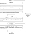Fig. 1

Schematic representation of steps followed by Cesam2k20 in computing a time step.

3 Opacity tables and equation of state

3.1 Opacity tables

Cesam2k20 implements numerical opacity tables issued by five different collaborations. The first ones are build by the OPAL team (Rogers & Iglesias 1992; Iglesias & Rogers 1996). They exist in two types: Type 1 opacity tables with fixed Z < 0.1; and Type 2 opacity tables, which also account for C and O enhancement. The latter are interpolated in Cesam2k20 with program z14xcotrin21.f written by A. I. Boothroyd⁴. The second ones come from the Opacity Project (OP; Seaton et al. 1994; Badnell et al. 2005; Seaton 2005, 2007), which offer access to mean opacities, monochromatic opacities and radiative accelerations. The OPAL and OP tables are supplemented at low temperatures by the Wichita⁵ opacity tables (Ferguson et al. 2005). They are also adapted to some of the main historical solar abundances determination. Table 1 summarises what is currently available. Above T = 7 · 10⁷ K, the plasma is considered fully ionised, and we only accounted for the Compton scattering by free electrons, evaluated using Poutanen (2017) fitting function, with a smooth transition between 7 · 10⁷ and 8.7 · 10⁷ K.

In addition to the opacity tables, the user can also choose how Cesam2k20 will interpolate in these tables. It is advised to use an interpolation scheme validated through the ESTA/CoRoT collaboration (see, e.g. Lebreton et al. 2008a; Montalbán et al. 2008). Recently, a new interpolation scheme, adapted from the xztrin21.f routine for Type 1 OPAL opacities⁶ has been added to Cesam2k20. It allows for smooth derivatives of the opacity, κ, to be obtained with respect to the temperature, T, or density, ρ, suitable for non-adiabatic oscillation computation. Interpolation routines using birational splines from G. Houdek OPALINT⁷ package are also provided (Houdek & Rogl 1996).

Table 1

Opacity tables available in Cesam2k20.

3.2 Conductive opacities

Conductive opacities can be computed in three different ways. Analytically, from expressions detailed in Iben (1975), or numerical by interpolating in tables, either from Cassisi et al. (2007); Potekhin et al. (2015) or the updated tables⁸ from Cassisi et al. (2021).

3.3 Equations of state

Several equations of state (EoS) are available with Cesam2k20 (see Table 2). Analytical EoSs are the same as the one presented in ML08. On the side of numerical EoSs, MHD tables (Hummer & Mihalas 1988; Mihalas et al. 1988) can still be used. Modern EoSs are also provided. The version of the OPAL 2005 EoS (Rogers & Nayfonov 2002) has been implemented. Recently, a collaborative effort has yielded to the integration of the SAHA-S EoS readily into Cesam2k20 (Baturin et al. 2017). The SAHA-S EoS (Gryaznov et al. 2006, 2013) is based on the chemical picture (Ebeling 1969) and solar models computed, which seems to be in better agreement with helioseismic data than the one computed with OPAL 2005 (which OPAL 2005 follows the physical picture; Vorontsov et al. 2013). SAHA-S is, at the moment, only adapted for 0.1 ≤ X ≤ 0.9, which prevents its use for stellar models beyond the main sequence or in specific cases, such as chemically peculiar stars with high hydrogen content at the surface. Routines adapted to SAHA-S are readily available in Cesam2k20 and the user should only download directly the data from the SAHA-S website⁹.

4 Convection

The modelling of convection is one of the major locks for our understanding of stellar structure and evolution. We thus carried many developments to improve the accuracy of the models. The two most important changes are (1) a new scheme for the determination of mixing region boundaries and (2) the possibility to have the convection parameter varying along evolution and physically constrained through the entropy calibration.

Table 2

Summary of the EoSs available in Cesam2k20.

4.1 Determination of limits with Gabriel et al. (2014)

One of the major improvements in this version of Cesam2k20 is the new method used to determine the convective boundaries. We define $d \nabla \equiv \nabla_{r a d} - \nabla_{a d} (+ \frac{φ}{δ} \nabla_{μ}),$ $\[\mathrm{d} \nabla \equiv \nabla_{\mathrm{rad}}-\nabla_{\mathrm{ad}}\left(+\frac{\varphi}{\delta} \nabla_\mu\right),\]$ (18)

the Schwarzschild’s criterion (Ledoux criterion if the term between parenthesis is added), where ∇_rad, ∇_ad, and ∇_μ are the radiative, adiabatic, and mean molecular weight gradients. Originally, CESTAM was computing the d∇ profile and between the two consecutive layers, where d∇ changes sign, the boundary is found by a linear interpolation. This process was repeated at each iteration during a given time step (see step 2 in Fig. 1). This technique was known to produce very erratic results, especially for models with a recessing convective core, where a mean molecular weight gradient has built up. In this case, d∇ becomes discontinuous at the boundary.

Figure 2 displays on the left a Kippenhahn diagram on which the dark grey region represents, for a 1.3 M_⊙ model called OrigM, the extent of the core CZ through time, as determined by the original method, and in light grey the RZ above it. From ~1.5 Gyrs to the vanishing of the core CZ, the location of the limit appears to be oscillating more and more. After ~3.0 Gyrs, we can even distinguish the temporary apparition of spurious CZ in red, just above the core CZ. These zones are only consequences of the numerical scheme, but have no physical meaning. The right panel shows the profiles of d∇, in dashed lines for OrigM, around the location of the limit CZ/RZ, for successive iterations performed during the computation of a time step. Grey arrows represent the location of the limit RZ/CZ at the ten previous time steps: in light grey, the location at the tenth previous time step, in dark grey at the immediate previous one. The method originally implemented in Cesam2k20 predicts a limit that does not decrease monotonically, for a convective core normally recessing at this stage of evolution

According to Gabriel et al. (2014) who examined in detail the possible misuses of boundary conditions, the location of the boundaries should not be found by looking for a change of sign d∇ between two consecutive layers by scanning from centre to surface. In case of a discontinuity, in the chemical composition, a change of sign can occur while the two layers are both radiative, both convective or radiative on one side, convective on the other. The only way to properly locate the boundary at d∇ = 0 is to always extrapolate from the interior of a convective zone. Gabriel et al. (2014) also advocates for the use of a double mesh point (two points located at the same mass coordinate: one in RZ and the other one in CZ), in case of a discontinuity. This was already implemented in CESAM and CESTAM as adding extra mesh points at discontinuities is part of the B-Spline machinery.

The limit of the core CZ/RZ for a 1.3 M_⊙ model called G14M obtained with the Gabriel et al. (2014) method is displayed in Fig. 2 (left panel). The extent of core CZ through time corresponds to the hatched region. The limit evolved in a much smoother way compared to what was obtained for OrigM. The right panel shows the profiles of d∇ for G14M in bold line through successive iterations at a given time step. The grey arrows show, as expected, that the boundary of the recessing core CZ is smoothly moving inwards through time. This new scheme is also more stable and converges faster than the original one. For the considered time step, convergence is reached after four iterations, while five were needed in the past. The new method is not without consequences for evolution. Because of the very erratic limit locations found with the old scheme, more hydrogen was injected from RZ to core CZ, thus prolonging the stellar lifetime. As an example, model OrigM reaches the TAMS (defined as central X reaching 0.01) at an age of 3740 Myrs, while model G14M reaches it at 3060 Myrs, a difference of around 20%.

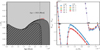Fig. 2

Left panel: Kippenhahn diagram of two models of 1.3 M_⊙ computed with the method originally implemented in CESAM (Morel 1997, hereafter model OrigM), and with the method prescribed by Gabriel et al. (2014, hereafter model G14M) and now implemented in Cesam2k20. The radiative zone corresponds to dark grey region for OrigM, and hatched region for G14M. Convective zone is the region in light grey for OrigM, and non-hatched region for G14M. Red regions are spurious convective zone. Vertical dashed line at age 2923 Myrs marks the position in time of the model represented on right. Right panel: profile of d∇ ≡ ∇_rad − ∇_ad as a function of the mass coordinate, m/M_⊙, at each iteration of a given time step (at age 2923 Myrs). Profiles for G14M are drawn in solid lines, and profiles for OrigM are in dashed lines. Up (G14M) or down (OrigM) triangles mark the location of each layer, at each iteration. Grey up (G14M) or down (OrigM) arrows mark the location of the convective boundary at the ten previous time steps. Lightest arrow if for the tenth previous time step and darkest arrow for the immediate previous one.

4.2 Entropy calibration

The issues with ad hoc models of convection used in 1D stellar evolution code have been known for some time and well studied, even if (at the moment) we lack better alternatives. For a detailed review of these problems, see Trampedach (2010) and for a review on convection modelling, see Kupka & Muthsam (2017). At the moment, the most widely used prescriptions for modelling convection are mixing length theory (MLT; Biermann 1932; Siedentopf 1935; Biermann 1942; Böhm-Vitense 1958), where the turbulence spectrum is reduced to a Dirac distribution (i.e. all convective flux is carried by one single eddy), and full spectrum of turbulence models (FST; Canuto & Mazzitelli 1991, 1992; Canuto et al. 1996) that approximate the turbulence spectrum with a Kolmogorov spectrum. As far as we know, Cesam2k20 is the only stellar evolution code with ATON Rome Stellar Evolution Code (Ventura et al. 1998) that implement all these models (see, Joyce & Tayar 2023). MLT and FST all rely on a free parameter called the convection parameter, α. Its definition slightly differs from one theory to the other, but its role is always to tune the properties of the convective flow so that the stellar model reproduces some observables. The choice of α has always been a challenge as it is not physically constrained. Yet its value strongly impact the evolutionary track and, in turn, stellar fundamental parameters estimates. Except in the case of a solar model where observable constraints are sufficiently tight to often ensure that a single value of α allows reproducing them, in case of other stars the solution is often degenerate. In addition, α is always assumed to be constant through time, while there is no good reason to think that properties of the convective flow should not vary across evolution.

To circumvent these issues, two approaches have been developed. The first one is to compute 1D stellar atmosphere models by tuning, among other parameters, α, to reproduce global properties of the 3D, more realistic, models of surface convection; for instance, the effective temperature T_eff, log g and [Fe/H]. Once a sufficient number of such 1D models have been obtained, it allows calibrating a function f(T_eff, log g, [Fe/H]) that fits the α values in the grid. Such a function can then readily be used in 1D stellar evolution codes to set the value of α for any tuple (T_eff, log g, [Fe/H]). This approach has been followed by Sonoi et al. (2019) who provide six fitting functions for six different set of microphysics, all implemented in Cesam2k20. With such a method, α is not fixed along evolution and its value is not a free parameter any more. However, a disadvantage is that the microphysics chosen to compute one’s model should match exactly the one used to compute the fitting function, which advocates for the second approach.

The second approach uses prescriptions for the value of the specific entropy of the adiabat of the convective envelope. Since the value of α directly determines on which adiabat the star is on, Spada et al. (2018); Spada & Demarque (2019); Spada et al. (2021) suggested to simply tune α along the evolution such that, at any time, the specific entropy of the adiabat of the 1D matches a prescribed value. This idea was implemented in Cesam2k20 and further tested by Manchon et al. (2024), who also explain how to correct the entropy prescriptions for different chemical compositions or choice of EoS, and they give recommendations on the use of prescriptions already provided by Ludwig et al. (1999); Magic et al. (2013); Tanner et al. (2016). This approach has several advantages over the first one. First, it relies on prescriptions for the specific entropy, which has a physical meaning, while α depends on the microphysics of the model. Second, it suppresses the need of choosing a poorly defined parameter when fitting a star, and allows either to remove a degree of freedom, or to calibrate an additional parameter that controls another physical process. Finally, EC modelling authorizes α to vary along evolution, which seems a strong approximation of the classical MLT modelling.

4.3 Overshoot

The effect of the overshoot is taken into account since the earliest version of CESAM. The overshooting regions were first assumed to be fully mixed and recently, the possibility to assume a diffusive mixing was added, according to the formulation of Herwig (2000), with the velocity scale height taken as H_v = α_ovH_p, where α_ov is the overshoot parameter and H_p the pressure scale height. In Cesam2k20, the overshoot parameters of the convective core (α_ov,c) and of the envelope (α_ov,e) can be controlled independently. The size of the overshooting region over the convective core is then min(α_ov,cH_p; R_cα_ov,c), with R_c the radius of the convective core, and is α_ov,eH_p below the convective envelope.

Several options can be chosen for setting the temperature gradient ∇ in the overshooting region. By default, we assume an adiabatic temperature gradient above the convective core, and a radiative gradient (or adiabatic if recommendation of Zahn 1991 are followed) below the convective envelope. Rempel (2004) show that these simple prescriptions lead to shallow overshooting regions, with sharp transitions in the temperature gradient, in contradiction with numerical simulation. To overcome this issue, Christensen-Dalsgaard et al. (2011) proposed an analytical expression for the temperature gradient in the overshoot region as $\nabla = \nabla_{a d} - \frac{2 F_{o v}}{β + \exp (2 ζ)},$ $\[\nabla=\nabla_{\mathrm{ad}}-\frac{2 \mathcal{F}_{\mathrm{ov}}}{\beta+\exp (2 \zeta)},\]$ (19)

where ℱ_ov, β, and ζ are certain quantities that control the shape of the transition (see Christensen-Dalsgaard et al. 2011 for details). This formulation allows to better reproduce the size of the penetrative convection region as inferred by helioseismology. However, for hotter stars, in which the radiative gradient does not decrease monotonically below the Schwarzschild’s boundary, a more complex form for ∇ can be considered, such as the one introduced by Deal et al. (2023): $\nabla = \nabla_{a d} - \frac{\nabla_{a d} - \nabla_{r a d}}{2} [1 - \frac{2}{π} \arctan (\frac{ζ (r) - α_{P C} H_{p} (r_{e})}{β {(\nabla_{a d} - \nabla_{r a d})}^{4}})],$ $\[\nabla=\nabla_{\mathrm{ad}}-\frac{\nabla_{\mathrm{ad}}-\nabla_{\mathrm{rad}}}{2}\left[1-\frac{2}{\pi} \arctan \left(\frac{\zeta(r)-\alpha_{\mathrm{PC}} H_p(r_{\mathrm{e}})}{\beta\left(\nabla_{\mathrm{ad}}-\nabla_{\mathrm{rad}}\right)^4}\right)\right],\]$ (20)

with ζ(r) = r − r_e, r_e being the radius of the Schwarzschild’s boundary of the convective envelope, α_PC is a tunable parameter, and β controls the steepness of the transition. All these options are available in Cesam2k20 for setting the gradient in the overshooting region.

5 Evolution of the chemical composition

From the first version of CESAM to the current Cesam2k20, a great deal of attention has been paid on the evolution of the chemical composition, and especially, the transport of chemical elements. This has contributed, over the years, to the acknowledgement of the chemical diffusion as being part of the standard model of stellar physics. The evolution of the concentration of an element X_i is governed by nuclear reactions and mixing processes such as convective motions, gravitational settling, radiative acceleration or MHD instability-induced mixing. This can be expressed by the following equation, $\begin{aligned} ρ \frac{\partial X_{i}}{\partial t} = & - λ_{i, nuc} ρ X_{i} - \frac{1}{r^{2}} \frac{\partial}{\partial r} (r^{2} ρ v_{i, H} X_{i}) \\ - \frac{1}{r^{2}} \frac{\partial}{\partial r} (r^{2} ρ D_{turb} \frac{\partial X_{i}}{\partial r}), \end{aligned}$ $\[\begin{aligned}\rho \frac{\partial X_i}{\partial t}= & -\lambda_{i, \text {nuc}} \rho X_i-\frac{1}{r^2} \frac{\partial}{\partial r}\left(r^2 \rho v_{i, \mathrm{H}} X_i\right) \\& -\frac{1}{r^2} \frac{\partial}{\partial r}\left(r^2 \rho D_{\text {turb}} \frac{\partial X_i}{\partial r}\right),\end{aligned}\]$ (21)

where λ_i,nuc is the nuclear reaction rate of specie i, v_i,H is the atomic diffusion velocity of specie i relative to hydrogen, and D_turb is a coefficient of diffusion associated with the turbulence. This general system of equations is solved using a relaxation technique (Press et al. 1995). Of course, if the user chooses to neglect atomic and turbulent diffusion, only the first term of the right-hand side remains.

5.1 New nuclear reaction rates

The nuclear reaction rates presented in ML08 are still available. In addition, the rates obtained from the compilations of NACRE II (Xu et al. 2013) – possibly supplemented with the rate of LUNA (Broggini et al. 2018) for the ¹⁴N(p, γ)¹⁵O reaction – or from the Reaclib database (Cyburt et al. 2010) can be chosen. With Cesam2k20, the user can only follow the evolution of elements that are part of a predefine nuclear networks, among which the user can choose the one that best suits their needs. The abundances of elements left out of the network are assumed to stay at equilibrium during evolution. These networks can account for reactions of the PP chains, CNO cycle or triple-α process with rates chosen from the above compilations. Screening effect can be included according to (Clayton 1968)’s prescription for weak screening (default) or following Mitler (1977)’s formalism. As mentioned in the introduction of this section, when atomic diffusion is neglected, Eq. (21) simplifies. In this case, the system is solved using an implicit Runge-Kutta type Lobatto IIIC integration scheme for stiff problems (see Hairer & Wanner 1996 or ML08 for more details).

5.2 Atomic diffusion

To compute atomic diffusion velocities, two formalisms are available. The first one consists in solving the full Burger’s equations for each element (Burgers 1969), and the second one, following Michaud & Proffitt (1993) amount to consider all elements other than hydrogen as test particles that only diffuse with respect to protons.

To the atomic diffusion velocities, one can add a contribution coming from the radiative accelerations. Cesam2k20 allows the use of the Single-Valued Parameter method (SVP; Alecian & LeBlanc 2002; Alecian & Leblanc 2004) or its update from Alecian & LeBlanc (2020). SVP method allows, in an optically thick medium, to separate the properties of the atoms and of the plasma. With such simplification, and assuming that the probabilities of bound-bound transitions (resp. bound-free transitions) have a Lorentzian profile (resp. Voigt profile), the expression for the radiative acceleration of a given element depends only on six parameters specific to the element, and its local abundance. This dramatically speeds up the computation with a small associated error.

5.3 Ad hoc turbulent diffusion prescriptions

The last term of Eq. (21) gathers all the contributions to the atomic diffusion induced by the turbulence. This includes known processes such as double diffusive convection (see Sect. 5.4) and rotation-induced mixing (see Sect. 6). Other options exist within Cesam2k20 to parametrise turbulent mixing with ad hoc prescriptions. Two of them, already available in later version of CESAM rely either on a coefficient calibrated below the Solar CZ (Gabriel 1997) or a fixed value used in regions where T < 10⁶ K, avoiding Helium’s sedimentation.

More recently, we have implemented other prescriptions. A first type of these have a turbulent diffusion coefficient of the form, $D_{turb} = ω D (H e)_{0} {(\frac{ρ_{0}}{ρ})}^{n},$ $\[D_{\text {turb }}=\omega D(\mathrm{He})_0\left(\frac{\rho_0}{\rho}\right)^n,\]$ (22)

where ω and n are two constants which can be set in the input file of Cesam2k20, D(He), and ρ are the local diffusion coefficient of Helium and density, while the subscript 0 indicates that the value is taken at a reference depth. This reference depth can be set at a given mass fraction or temperature (prescription of Richer et al. 2000) or at the base of the convective zone (see the prescription of Proffitt & Michaud 1991). The reference depth can also be varied between two calibrated reference values that allow us, for example, to reproduce the helium abundance of F-type stars (Verma & Silva Aguirre 2019) and the Li⁷ of the Sun, following an idea applied in Moedas et al. (2025). The second type of prescription (Freytag et al. 1996; Théado et al. 2009; Deal et al. 2016, 2018) takes the following form, $D_{turb} = ω_{1} \exp (\frac{r - r_{e}}{σ_{1} R} \ln 2) + ω_{2} \exp (\frac{r - r_{e}}{σ_{2} R} \ln 2),$ $\[D_{\text {turb}}=\omega_1 ~\exp \left(\frac{r-r_{\mathrm{e}}}{\sigma_1 R} ~\ln~ 2\right)+\omega_2 ~\exp \left(\frac{r-r_{\mathrm{e}}}{\sigma_2 R} ~\ln~ 2\right),\]$ (23)

where ω₁, ω₂, σ₁ and σ₂ are user-defined constants, and r_e was already defined in Eq. (20).

5.4 Double diffusive convection

To this ad hoc treatment of turbulent diffusion, Cesam2k20 is also able to include the effect of specific physical mechanisms, namely, the thermohaline convection or the semi-convection. The first one is triggered in the region where the medium is stable with respect to the thermal gradient, but it is unstable because of the gradient of mean molecular weight. Thus, it is treated using the formalism ofrom Brown et al. (2013). The other is triggered when opposite conditions are met and Cesam2k20 models it following Langer et al. (1983).

6 Evolution of the angular momentum distribution

6.1 Angular momentum transport according to Zahn (1992)

The treatment of angular momentum transport according to Zahn (1992) in Cesam2k20 is described in M13. We recall the general ideas and then report on the new, non-standard developments. Angular momentum is globally conserved in a Cesam2k20 model except that it can be gained at the surface through planetoid infall (see ML08), or lost at the surface through magnetized stellar winds. While the analytical model of Kawaler (1988) is still available, Cesam2k20 now offer the possibility to use a scaling relation derived from 3D simulation of magnetized stellar winds (Matt et al. 2015), which assumes a more complex geometry of the magnetic field.

In the interior, the treatment of the transport of angular momentum (TAM) is different whether we are in a convective or radiative zone. Inside the former, because of the efficient mixing, we can assume uniform distribution of the angular velocity (solid body rotation), or of the angular momentum (local conservation of angular momentum). Inside a radiative zone, we use the framework of Zahn (1992) and Talon et al. (1997). First, large scale meridional currents are needed to verify baroclinic equilibrium. This meridional circulation advects angular momentum 𝒥 and chemical elements. Second, shear-induced turbulence (Kelvin-Helmoltz instability) diffuses angular velocity Ω. Third, since this viscosity is much stronger horizontally than vertically, we assume that the radiative zone is in shellular rotation, namely, Ω depends only on the radial coordinate. The TAM is then modelled in Cesam2k20 as an advecto-diffusive process. The latitudinal variations are decomposed as a series of Legendre polynomials, and degrees ℓ > 2 are neglected. Hence, the angular momentum transported vertically follows $ρ \frac{d r^{2} Ω}{d t} = \frac{1}{5 r^{2}} \frac{\partial}{\partial r} (ρ r^{4} Ω U_{2}) + \frac{1}{r^{2}} \frac{\partial}{\partial r} (ρ ν_{ν} r^{4} \frac{\partial Ω}{\partial r}),$ $\[\rho \frac{\mathrm{d} r^2 \Omega}{\mathrm{~d} t}=\frac{1}{5 r^2} \frac{\partial}{\partial r}\left(\rho r^4 \Omega U_2\right)+\frac{1}{r^2} \frac{\partial}{\partial r}\left(\rho \nu_{\mathrm{\nu}} r^4 \frac{\partial \Omega}{\partial r}\right),\]$ (24)

where U₂ is the vertical component of the meridional circulation, and ν_v is the vertical shear-induced viscosity coefficient. Equation (24) is solved with the linear two-point boundary relaxation method described in Press et al. (1995). Coefficients of the differential equations are computed explicitly with the solution of the structure found at previous iteration. Many prescriptions have been suggested to provide a value for the diffusion coefficients of the Kelvin-Helmholtz instability, either from theoretical considerations or experiments. Cesam2k20 implements three of them as proposed in Palacios et al. (2003); Mathis et al. (2004) and Mathis et al. (2018).

The effect of the TAM on the transport of chemicals is accounted for through an additional term of the right-hand side of Eq. (21), expressed as $\frac{1}{r^{2}} \frac{\partial}{\partial r} [r^{2} ρ (D_{v} + D_{e f f}) \frac{\partial X_{i}}{\partial r}],$ $\[\frac{1}{r^2} \frac{\partial}{\partial r}\left[r^2 \rho\left(D_{\mathrm{v}}+D_{\mathrm{eff}}\right) \frac{\partial X_i}{\partial r}\right],\]$ (25)

where D_v = ν_v and D_eff = (rU₂)²/(30D_h), with D_h the horizontal shear-induced viscosity coefficient.

Finally, to initialize the distribution of angular momentum, we make use of the disc-locking model. As suggested by Bouvier et al. (1997), young, completely convective, fast-rotating stars have strong magnetic fields that lock the convective zone with the accretion disc. Then, the convective envelope of the star is forced to co-rotate with the accretion disc, as long as it exists. With only two parameters being the rotation period, P_disc, and its lifetime, τ_disc, this model provides a simple initial distribution of angular momentum.

6.2 Additional transport mechanisms

It has been known for more than a decade that this model fails to reproduce the flat internal rotation profile of the solar radiative zone derived from helioseismology. The core rotation of subgiant and red giant stars derived from asteroseismic observations also strongly disagrees with the model’s predictions (e.g. Eggenberger et al. 2012; Marques et al. 2013; Goupil et al. 2013b; Cantiello et al. 2014; Fuller et al. 2014; Ouazzani et al. 2019). Several mechanisms have been suggested to explain the missing TAM. These mechanisms fall into two categories: either angular momentum advected by waves, or a diffusion of angular velocity by (magneto)hydrodynamic instabilities. At the moment, none of them is found to solve the TAM problem alone.

Cesam2k20 can account for the angular momentum transported by mixed-modes, following the idea developed by Belkacem et al. (2015b,a). This is done by adding a flux term −1/r²∂(r²ℱ_waves)/∂r in the right-hand side of (24). While Belkacem et al. (2015a) computed the fluxes a posteriori for a few models, with eigenfunctions computed using ADIPLS (Christensen-Dalsgaard 2008a), transport by mixed-modes can now be computed throughout the evolution, using asymptotic expression for eigenfrequencies and eigenfunctions, as well as a scaling relation for the amplitude of the eigenmodes (e.g. Mosser et al. 2010; Samadi 2011; Belkacem & Samadi 2013; Benomar et al. 2014).

On the side of (magneto)hydrodynamic instabilities, two of them have been recently added or improved in Cesam2k20. First, the Goldreich-Schubert-Fricke (GSF) instability (Goldreich & Schubert 1967; Fricke 1968; Acheson & Gibbons 1978), which is purely hydrodynamical, occurs when the shear perpendicular to the rotation axis is strong enough to overcome the stabilizing effect of the thermal and chemical stratifications. In addition to the model that already existed in CESTAM (see M13), we now also propose to use the GSF coefficient of angular momentum diffusion obtained from scaling relations extracted from results of 2D simulations of GSF instability near the stellar equator presented in Barker et al. (2019).

The Tayler instability (TI) is thought, at the moment, to be among the most efficient MHD instability at transporting angular momentum. The latest version of CESTAM already included the TI, following the analytical formalism of Spruit (2002) generalised by Maeder & Meynet (2004). Due to very short timescale of diffusion of angular velocity compared to the timescale of the evolution of the structure, TI is known to induce numerical errors (see e.g. Yoon & Langer 2004; Neunteufel et al. 2017; Wheeler et al. 2015). Recently, new analytical model of TI as proposed by Fuller et al. (2019) or scaling relations derived by Daniel et al. (2023) from 3D MHD simulations have been added to Cesam2k20. Moreover, a lot of effort have been put into improving its implementation and this will be the topic of a forthcoming paper. With the current version of Cesam2k20, models including the TI as a transport process will produce angular velocity profiles that might be reliable qualitatively but are still impacted by numerical artefacts.

Table 3

Summary of T(τ) relations available in Cesam2k20.

7 Atmosphere

The details of the implementation of atmosphere reconstruction in Cesam2k20 have already been described in ML08, and even more precisely in Morel et al. (1994). Two possibilities exists to model the atmosphere: using a T(τ) relation or interpolation into a pre-computed grid of stellar atmospheres.

7.1 New purely-radiative T(τ) relations

In the atmosphere, the system of structure equations can be rewritten with the optical depth, τ, as the reference coordinate. To close the system, the temperature profile can be set through a T(τ) relation, $T (τ) = T_{e f f} {[\frac{3}{4} (q (τ) + τ)]}^{1 / 4},$ $\[T(\tau)=T_{\mathrm{eff}}\left[\frac{3}{4}(q(\tau)+\tau)\right]^{1 / 4},\]$ (26)

where q(τ) is the Hopf function, the value of which must be prescribed. Three new T(τ) relations have been added to the new version of Cesam2k20 (see. Table 3. The first two, derived by Krishna Swamy (1966) and Vernazza et al. (1981), are constructed to reproduce, respectively, observations of K dwarfs, and of the Sun’s photosphere (called VAL-C model). The last T(τ) relation has a functional form suggested by Ball (2021), and is calibrated on a 3D simulation of the Sun (Trampedach et al. 2014). Its behaviour is quite similar to the VAL-C model for large τ, but reproduce better the shape of q(τ) ∝ log τ in the limit of τ → 0.

7.2 Non-purely-radiative T(τ) relations

Non-purely-radiative T(τ) relations are the same as the one already mentioned in ML08 paper, only the corresponding tables have been updated. Several routines based on the Kurucz’s ATLAS9 non-radiative model atmospheres (see, e.g, Kurucz 2014, and their description of the different versions of ATLAS models and references therein) were originally written to model the atmosphere of the Sun (see e.g. Morel et al. 1994), but are no longer used. Then, a more general routine rogerYL has been designed to allow interpolation within a large set of T(τ) laws derived from ATLAS12 models. These laws cover the range 3500 K < T_eff < 7000 K and 1 < log g < 5 and are provided for a solar mixture and four values of [Fe/H] (−1.0, −0.5, +0.0, +0.2, for the value −1.0 the law takes into account an α-element enrichment of +0.4 characteristic of low metallicity stars). In a former version of CESAM, T(τ) laws from the MARCS (Gustafsson et al. 2008) and PHOENIX (Allard 2014) model atmospheres have been implemented; they will soon be available in the present version.

Table 4

Summary of mass-loss recipes available in Cesam2k20.

8 Stellar mass loss

Very recently, a lot of work has been put into better describing the mass loss in stellar models. Cesam2k20 implements eight different mass-loss prescriptions and can switch from one to the other along the evolution. The most simple prescriptions involve a constant mass loss (or gain), $\dot{M}$ $\[\dot{M}\]$ . More complex ones are derived from observations or 3D simulations. A brief summary of available options is given in Table 4.

Apart from simple recipes, which account for a constant mass loss or gain during part or the entire lifetime of the star, all others implemented in Cesam2k20 follow a Reimers-like law Reimers (1975), expressed as $\dot{M} \propto η \frac{L R}{M},$ $\[\dot{M} \propto \eta \frac{L R}{M},\]$ (27)

where η is a proportionality factor that should be the same for different stars and different evolutionary status, L is the luminosity, R the radius, and M the mass. In the original formulation by Reimers (1975), η was actually found to vary with stellar mass and evolutionary stage. Later works slightly changed this original formulation to obtain a constant η (Schröder & Cuntz 2005; Rosenfield et al. 2014). In the end, it seems that a better approach is to switch from one formulation to the other as the star gets older, which is now allowed in Cesam2k20.

9 Application: Solar models

To demonstrate the abilities of Cesam2k20, we computed a series of standard and non-standard solar models. We did not choose to show examples of all the new options, but, rather, we illustrate the main progresses of the code. These models are computed with the help of the OSM package¹⁰, that finds the Cesam2k20 model that best matches a set of observational constraints, by tuning a set of adjustable parameters, following a Levenberg-Marquardt algorithm. The set of these parameters varies from one model to the other, as well as the numerical precision, and the input physics.

9.1 Physical inputs

Common physical ingredients. All models were stopped at the same age, 4570 Myrs and computed with the same reference composition ratios of Asplund et al. (2021, hereafter AAG21), following the ‘meteoritic’ compilation, EoS (OPAL 2005), opacities (OPAL adapted to the AAG21), and MLT. The adopted preset numerical precision are named after the space-borne mission for which they were tailored: ‘co’ for CoRoT and ‘pl’ for PLATO. Thanks to more modern computational resources, the PLATO precision is higher than the CoRot one. In particular, it introduces more shells and more time-steps during evolution. We describe below the main characteristics of the solar models. These are summarised in Table 5, while the set of observational constraints and the optimal values of tunable parameters are listed in Tables 6 and 7.

SSM1. The first standard solar model (SSM1) presented here is the model obtained with the default physics and numerical settings of Cesam2k20 (‘co’). It includes the physical ingredients described in Sect. 9.1, with no diffusion of chemical elements, nor any transport of angular momentum. Its initial Helium abundance, Y₀, and parameter α_MLT of MLT are calibrated so that it reproduces the solar T_eff and luminosity.

SSM2. The second standard solar model (SSM2) is computed with the choice of input physics made to compute the first generation grid of stellar models for the PLATO mission, except that the convection is modelled with a traditional MLT with fixed α_MLT, and is not entropy-calibrated. The numerical precision is higher (‘pl’) and gravitational settling as well as turbulent mixing of chemical elements are included. The turbulent diffusion coefficient follows Eq. (22), with ω = 10⁴, n = 4 and the reference depth is set at a mass of 5 · 10⁴ below the surface. This choice is more suitable for F-type stars, and induces little mixing in the Sun. The treatment of turbulent diffusion shall be improved for the second generation of the grid. Contrary to SSM1, the atmosphere is here reconstructed with T(τ) relation of Vernazza et al. (1981), which was calibrated to reproduce solar temperature gradient in the photosphere. To the previous choice of constraints and tunable parameters, we also tuned the initial Z/X ratio and the overshoot parameter below the convective envelope to reproduce present solar Z/X at the surface, and the acoustic travel time in the convective envelope.

NSSM1. In a first non-standard model (NSSM1), we replace additional turbulent mixing adapted to F-type stars to a calibrated one. This mixing is still described by Eq. (22), but ω = 400 and n = 3. The reference depth, in the present case located by a temperature T_mix, is tuned, so that our model reproduces the present surface ⁷Li abundance of the Sun. We also kept Y₀, (Z/X)₀, and α_MLT as tunable parameters and T_eff, L, and (Z/X)_s as observational constraints. For all non-standard models here, the overshoot below the envelope is turned off and the atmosphere follows the T(τ) relation from Vernazza et al. (1981).

NSSM2. Then, NSSM2 has the same settings as SSM2 for the turbulent diffusion, however, rotation is taken into account following the Talon et al. (1997) formalism as well as including the Matt et al. (2015)’s prescription for the loss of angular momentum by magnetized solar winds. This scaling relation depends on a multiplicative parameter T₀ = 9.5 × 10³⁰ in the original paper. We took it as a free parameter and made it vary so that we recover the surface solar rotation age at present age. The period and lifetime of the disk are set to 10 days and 5 Myrs, for lack of a better choice.

NSSM3. Finally, the last non-standard model (NSSM3) combines the above two transport processes. These are controlled by T_mix and T₀.

Table 5

Physical ingredients of the standard and non-standard solar models.

Table 6

Values of observational constraints used to produce each calibrated solar models.

9.2 Acoustic structure

A classical test for assessing the accuracy of the structure of solar model is to compare the modelled sound speed c_s,mdl to the sound speed profile inverted using helioseismology c_s,obs. For this reference profile, we used the data provided by Basu et al. (2000) inverted using frequency measurements of the Michelson-Doppler Imager (MDI) on-board Solar and Heliospheric Observatory (SoHO) satellite (Scherrer et al. 1995). The relative difference c_s,mdl and c_s,obs are displayed in Fig. 3, left panel. The highest relative differences reach 2% for the simplest standard, SSM1, around 0.6 R_⊙. It should be stressed that the peak is higher, but comparable to what was shown in Fig. 1 of ML08 (1.5%) with the previous version CESAM 2 k. This model was computed with the solar chemical composition of Asplund et al. (2005, AGS05) and the microscopic diffusion of MP93, while SSM1 used AAG21 and no diffusion. These different choices of modelling somewhat compensate each other: AGS05 is known to lo lead to inaccurate sound speed in the interior (see e.g. Asplund et al. 2009), while accounting for the microscopic diffusion lower the error on the sound speed. The other three models (SSM2 and NSSM1-3) have display comparable error on their sound speed profiles. Their maximum error is still higher than what was shown in ML08. The reason is again that the solar abundance determinations from Grevesse & Noels (1993) were used for the best models of ML08, which are known to lead to better agreement with inverted sound speed than when using AAG21 as it is the case for the models of the present paper (see e.g. Buldgen et al. 2019).

We note that a better agreement with the sound speed profile is not a sufficient criterion to make a better solar model (Eggenberger et al. 2022; Buldgen et al. 2024, 2025). Of all the models, the standard SSM2 model has the most accurate sound speed profile, while it does not incorporate the most complex physical ingredients. These models should be tested against other constraints than just their ability at reproducing the sound speed.

Table 7

Values of tunable parameters obtained after the calibration of each solar models.

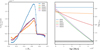Fig. 3

Left panel: relative differences between inverted and modelled sound speed as a function of the radial coordinate, for SSM1 to NSSM3. The inverted sound speed is taken from (Basu et al. 2000). Right panel: time evolution of the surface ⁷Li abundance for SSM1 to NSSM3. Horizontal black line is the present-day solar surface ⁷Li abundance as measured by Asplund et al. (2021), and the shaded area represents the associated uncertainty.

9.3 Lithium abundance

In Fig. 3, we display on the right panel the evolution of the surface ⁷Li abundance, as well as the targeted value. It is clear that we can no longer be satisfied with the standard model, even when it includes microscopic diffusion as SSM2. Indeed, almost no ⁷Li is depleted from the formation of the star to the present age of the Sun. The model NSSM2 that includes rotation, but no additional turbulent transport depletes more ⁷Li thanks to the enhanced transport of chemical elements brought by the shear-induced turbulence and the stronger coupling between the radiative zone and the convective envelope. However, the only way to achieve the present-day surface solar ⁷Li abundance is by adding an extra mechanism for the transport of the chemical elements. In Cesam2k20, this can be done though an ad hoc turbulent mixing as it is the case in SSM1 and SSM3, but it could also be done by adding new processes like waves of (M)HD instabilities, similarly to models present in the literature (e.g. Talon & Charbonnel 2003; Fuller et al. 2015; Eggenberger et al. 2019a,b).

10 Conclusion

In this paper, we present the main aspects of the numerical machinery, covering the most recent developments regarding the physical processes that Cesam2k20 has the capacity to include and that were not available in earlier versions of CESAM or CESTAM. We have shown, through a series of standard and non-standard solar models, the capabilities of Cesam2k20 for reproducing the acoustic structure of the Sun or the present-day surface solar ⁷Li abundance. Currently, progress is also being made in the modelling of (M)HD instabilities, carrying angular momentum or chemical elements, in terms of the impact of magnetic fields on the stellar structure and evolution, on the reconstruction of atmospheres, and on other features.

Recently, part of this overall effort has opened Cesam2k20 up to the community. We built a website¹¹ that puts togethr a ‘quick start’ guide, an improved documentation that is progressively being translated into English. On this website, we provide some models, in particular, all the models presented in this work, along with a link to the public repository. The public version will be updated regularly, with new published developments and bug fixing. The code is licensed under GPLv3, which means that the code can be changed, shared, or used for commercial use, as long as the source is made available with the same licence.

Acknowledgements

The authors warmly thanks everybody who played a role, even the tiniest, in the development of Cesam2k20 and earlier versions over the years, in particular Pierre Morel. The authors also thank A. Oreshina, V. Baturin, and all the people behind the SAHA-S EoS for their help in implementing it in Cesam2k20. L.M. acknowledge support from the Agence Nationale de la Recherche (ANR) grant ANR-21-CE31-0018 and from the Max Planck Society (MPG) under project “Preparations for PLATO Science”. M.D. acknowledge the support from CNES, focused on PLATO.

References

Acheson, D. J., & Gibbons, M. P. 1978, Phil. Trans. R. Soc. London Ser. A, 289, 459 [CrossRef] [Google Scholar]
Aerts, C., Mathis, S., & Rogers, T. M. 2019, ARA&A, 57, 35 [Google Scholar]
Alecian, G., & LeBlanc, F. 2002, MNRAS, 332, 891 [NASA ADS] [CrossRef] [Google Scholar]
Alecian, G., & Leblanc, F. 2004, IAU Symp., 224, 587 [Google Scholar]
Alecian, E., & Lebreton, Y. 2020, in Stellar Magnetism: A Workshop in Honour of the Career and Contributions of John D. Landstreet, ed. G. Wade, E. Alecian, D. Bohlender, & A. Sigut, 11, 125 [NASA ADS] [Google Scholar]
Alecian, G., & LeBlanc, F. 2020, MNRAS, 498, 3420 [NASA ADS] [CrossRef] [Google Scholar]
Alecian, E., Goupil, M. J., Lebreton, Y., Dupret, M. A., & Catala, C. 2007a, A&A, 465, 241 [NASA ADS] [CrossRef] [EDP Sciences] [Google Scholar]
Alecian, E., Lebreton, Y., Goupil, M. J., Dupret, M. A., & Catala, C. 2007b, A&A, 473, 181 [NASA ADS] [CrossRef] [EDP Sciences] [Google Scholar]
Alecian, E., Wade, G. A., Catala, C., et al. 2009, MNRAS, 400, 354 [CrossRef] [Google Scholar]
Allard, F. 2014, IAU Symp., 299, 271 [Google Scholar]
Amado, P. J., Moya, A., Suárez, J. C., et al. 2004, MNRAS, 352, L11 [Google Scholar]
Appourchaux, T., Antia, H. M., Ball, W., et al. 2015, A&A, 582, A25 [NASA ADS] [CrossRef] [EDP Sciences] [Google Scholar]
Asplund, M., Grevesse, N., & Sauval, A. J. 2005, ASP Conf. Ser., 336, 25 [Google Scholar]
Asplund, M., Grevesse, N., Sauval, A. J., & Scott, P. 2009, ARA&A, 47, 481 [NASA ADS] [CrossRef] [Google Scholar]
Asplund, M., Amarsi, A. M., & Grevesse, N. 2021, A&A, 653, A141 [NASA ADS] [CrossRef] [EDP Sciences] [Google Scholar]
Badnell, N. R., Bautista, M. A., Butler, K., et al. 2005, MNRAS, 360, 458 [Google Scholar]
Baglin, A., Auvergne, M., Barge, P., et al. 2006, ESA SP, 1306, 33 [NASA ADS] [Google Scholar]
Ball, W. H. 2021, Res. Notes Am. Astron. Soc., 5, 7 [NASA ADS] [Google Scholar]
Ballot, J., Turck-Chièze, S., & García, R. A. 2004, A&A, 423, 1051 [NASA ADS] [CrossRef] [EDP Sciences] [Google Scholar]
Barker, A. J., Jones, C. A., & Tobias, S. M. 2019, MNRAS, 487, 1777 [Google Scholar]
Basu, S., Pinsonneault, M. H., & Bahcall, J. N. 2000, ApJ, 529, 1084 [NASA ADS] [CrossRef] [Google Scholar]
Baturin, V. A., Däppen, W., Morel, P., et al. 2017, A&A, 606, A129 [NASA ADS] [CrossRef] [EDP Sciences] [Google Scholar]
Baudin, F., Barban, C., Goupil, M. J., et al. 2012, A&A, 538, A73 [NASA ADS] [CrossRef] [EDP Sciences] [Google Scholar]
Beck, J. G. 2000, Sol. Phys., 191, 47 [NASA ADS] [CrossRef] [Google Scholar]
Belkacem, K., & Samadi, R. 2013, Lecture Notes Phys., 865, 179 [Google Scholar]
Belkacem, K., Samadi, R., Goupil, M. J., & Dupret, M. A. 2008, A&A, 478, 163 [NASA ADS] [CrossRef] [EDP Sciences] [Google Scholar]
Belkacem, K., Samadi, R., Goupil, M. J., et al. 2009, A&A, 494, 191 [NASA ADS] [CrossRef] [EDP Sciences] [Google Scholar]
Belkacem, K., Marques, J. P., Goupil, M. J., et al. 2015a, A&A, 579, A31 [NASA ADS] [CrossRef] [EDP Sciences] [Google Scholar]
Belkacem, K., Marques, J. P., Goupil, M. J., et al. 2015b, A&A, 579, A30 [NASA ADS] [CrossRef] [EDP Sciences] [Google Scholar]
Benomar, O., Belkacem, K., Bedding, T. R., et al. 2014, ApJ, 781, L29 [Google Scholar]
Berthomieu, G., Provost, J., Morel, P., & Lebreton, Y. 1993, A&A, 268, 775 [NASA ADS] [Google Scholar]
Biermann, L. 1932, PhD thesis, Georg August University of Gottingen, Germany [Google Scholar]
Biermann, L. 1942, ZAp, 21, 320 [NASA ADS] [Google Scholar]
Böhm-Vitense, E. 1958, Z. Astrophys., 46, 108 [Google Scholar]
Bouvier, J., Forestini, M., & Allain, S. 1997, A&A, 326, 1023 [NASA ADS] [Google Scholar]
Bressan, A., Fagotto, F., Bertelli, G., & Chiosi, C. 1993, A&AS, 100, 647 [NASA ADS] [Google Scholar]
Bressan, A., Marigo, P., Girardi, L., et al. 2012, MNRAS, 427, 127 [NASA ADS] [CrossRef] [Google Scholar]
Broggini, C., Bemmerer, D., Caciolli, A., & Trezzi, D. 2018, Prog. Part. Nucl. Phys., 98, 55 [CrossRef] [Google Scholar]
Brown, J. M., Garaud, P., & Stellmach, S. 2013, ApJ, 768, 34 [NASA ADS] [CrossRef] [Google Scholar]
Brun, A. S., Turck-Chièze, S., & Morel, P. 1998, ApJ, 506, 913 [Google Scholar]
Brun, A. S., Turck-Chièze, S., & Zahn, J. P. 1999, ApJ, 525, 1032 [Google Scholar]
Buldgen, G., Salmon, S. J. A. J., Noels, A., et al. 2019, A&A, 621, A33 [NASA ADS] [CrossRef] [EDP Sciences] [Google Scholar]
Buldgen, G., Noels, A., Scuflaire, R., et al. 2024, A&A, 686, A108 [NASA ADS] [CrossRef] [EDP Sciences] [Google Scholar]
Buldgen, G., Noels, A., Amarsi, A. M., et al. 2025, A&A, 694, A285 [NASA ADS] [CrossRef] [EDP Sciences] [Google Scholar]
Burgers, J. M. 1969, Flow Equations for Composite Gases (Amsterdam: Elsevier) [Google Scholar]
Campilho, B., Deal, M., & Bossini, D. 2022, A&A, 659, A162 [NASA ADS] [CrossRef] [EDP Sciences] [Google Scholar]
Cantiello, M., Mankovich, C., Bildsten, L., Christensen-Dalsgaard, J., & Paxton, B. 2014, ApJ, 788, 93 [Google Scholar]
Canuto, V. M., & Mazzitelli, I. 1991, ApJ, 370, 295 [NASA ADS] [CrossRef] [Google Scholar]
Canuto, V. M., & Mazzitelli, I. 1992, ApJ, 389, 724 [NASA ADS] [CrossRef] [Google Scholar]
Canuto, V. M., Goldman, I., & Mazzitelli, I. 1996, ApJ, 473, 550 [NASA ADS] [CrossRef] [Google Scholar]
Casanellas, J., Brandão, I., & Lebreton, Y. 2015, Phys. Rev. D, 91, 103535 [Google Scholar]
Casanellas, J., & Lopes, I. 2011, ApJ, 733, L51 [Google Scholar]
Casas, R., Suárez, J. C., Moya, A., & Garrido, R. 2006, A&A, 455, 1019 [NASA ADS] [CrossRef] [EDP Sciences] [Google Scholar]
Cassisi, S., Potekhin, A. Y., Pietrinferni, A., Catelan, M., & Salaris, M. 2007, ApJ, 661, 1094 [NASA ADS] [CrossRef] [Google Scholar]
Cassisi, S., Potekhin, A. Y., Salaris, M., & Pietrinferni, A. 2021, A&A, 654, A149 [NASA ADS] [CrossRef] [EDP Sciences] [Google Scholar]
Castro, M., Baudin, F., Benomar, O., et al. 2021, MNRAS, 505, 2151 [NASA ADS] [CrossRef] [Google Scholar]
Cayrel de Strobel, G., Lebreton, Y., Soubiran, C., & Friel, E. D. 1999, Ap&SS, 265, 345 [Google Scholar]
Cayrel, R., Perrin, M. N., Lebreton, Y., Baglin, A., & Fernandes, J. 2000, in Liege International Astrophysical Colloquia, Vol. 35, Liege International Astrophysical Colloquia, eds. A. Noels, P. Magain, D. Caro, E. Jehin, G. Parmentier, & A. A. Thoul, 459 [Google Scholar]
Chapellier, E., Mathias, P., Garrido, R., et al. 2004, A&A, 426, 247 [NASA ADS] [CrossRef] [EDP Sciences] [Google Scholar]
Chaplin, W. J., Serenelli, A. M., Miglio, A., et al. 2020, Nat. Astron., 4, 382 [Google Scholar]
Christensen-Dalsgaard, J. 1982, MNRAS, 199, 735 [Google Scholar]
Christensen-Dalsgaard, J. 1988, Computational procedures for GONG solar model project, Astronomisk Institut, Aarhus Universitet [Google Scholar]
Christensen-Dalsgaard, J. 2008a, Ap&SS, 316, 113 [Google Scholar]
Christensen-Dalsgaard, J. 2008b, Ap&SS, 316, 13 [Google Scholar]
Christensen-Dalsgaard, J., & Daeppen, W. 1992, A&A Rev., 4, 267 [NASA ADS] [CrossRef] [Google Scholar]
Christensen-Dalsgaard, J., Monteiro, M. J. P. F. G., Rempel, M., & Thompson, M. J. 2011, MNRAS, 414, 1158 [CrossRef] [Google Scholar]
Christensen-Dalsgaard, J., Silva Aguirre, V., Cassisi, S., et al. 2020, A&A, 635, A165 [NASA ADS] [CrossRef] [EDP Sciences] [Google Scholar]
Clayton, D. D. 1968, Principles of Stellar Evolution and Nucleosynthesis (Chicago: University of Chicago Press) [Google Scholar]
Cordier, D., Lebreton, Y., Goupil, M. J., et al. 2002, A&A, 392, 169 [NASA ADS] [CrossRef] [EDP Sciences] [Google Scholar]
Cordier, D., Goupil, M. J., & Lebreton, Y. 2003, A&A, 409, 491 [NASA ADS] [CrossRef] [EDP Sciences] [Google Scholar]
Couvidat, S., Turck-Chièze, S., & Kosovichev, A. G. 2003, ApJ, 599, 1434 [Google Scholar]
Crida, A., Ligi, R., Dorn, C., & Lebreton, Y. 2018, ApJ, 860, 122 [NASA ADS] [CrossRef] [Google Scholar]
Cunha, M. S. 2006, MNRAS, 365, 153 [NASA ADS] [CrossRef] [Google Scholar]
Cyburt, R. H., Amthor, A. M., Ferguson, R., et al. 2010, ApJS, 189, 240 [NASA ADS] [CrossRef] [Google Scholar]
Daniel, F., Petitdemange, L., & Gissinger, C. 2023, Phys. Rev. Fluids, 8, 123701 [NASA ADS] [CrossRef] [Google Scholar]
De Boor, C. 2001, A Practical Guide to Splines, Applied mathematical sciences (Berlin: Springer) [Google Scholar]
de Bruijne, J. H. J., Hoogerwerf, R., & de Zeeuw, P. T. 2001, A&A, 367, 111 [NASA ADS] [CrossRef] [EDP Sciences] [Google Scholar]
Deal, M., Richard, O., & Vauclair, S. 2016, A&A, 589, A140 [NASA ADS] [CrossRef] [EDP Sciences] [Google Scholar]
Deal, M., Alecian, G., Lebreton, Y., et al. 2018, A&A, 618, A10 [NASA ADS] [CrossRef] [EDP Sciences] [Google Scholar]
Deal, M., Goupil, M. J., Cunha, M. S., et al. 2023, A&A, 673, A49 [NASA ADS] [CrossRef] [EDP Sciences] [Google Scholar]
Deheuvels, S., Bruntt, H., Michel, E., et al. 2010a, A&A, 515, A87 [NASA ADS] [CrossRef] [EDP Sciences] [Google Scholar]
Deheuvels, S., Michel, E., Goupil, M. J., et al. 2010b, A&A, 514, A31 [NASA ADS] [CrossRef] [EDP Sciences] [Google Scholar]
Deheuvels, S., Brandão, I., Silva Aguirre, V., et al. 2016, A&A, 589, A93 [NASA ADS] [CrossRef] [EDP Sciences] [Google Scholar]
Dintrans, B., & Rieutord, M. 2000, A&A, 354, 86 [NASA ADS] [Google Scholar]
Ebeling, W. 1969, Physica, 43, 293 [Google Scholar]
Eggenberger, P., Meynet, G., Maeder, A., et al. 2008, Ap&SS, 316, 43 [Google Scholar]
Eggenberger, P., Montalbán, J., & Miglio, A. 2012, A&A, 544, L4 [NASA ADS] [CrossRef] [EDP Sciences] [Google Scholar]
Eggenberger, P., Deheuvels, S., Miglio, A., et al. 2019a, A&A, 621, A66 [NASA ADS] [CrossRef] [EDP Sciences] [Google Scholar]
Eggenberger, P., den Hartogh, J. W., Buldgen, G., et al. 2019b, A&A, 631, L6 [NASA ADS] [CrossRef] [EDP Sciences] [Google Scholar]
Eggenberger, P., Buldgen, G., Salmon, S. J. A. J., et al. 2022, Nat. Astron., 6, 788 [NASA ADS] [CrossRef] [Google Scholar]
Eggleton, P. P., Faulkner, J., & Flannery, B. P. 1973, A&A, 23, 325 [NASA ADS] [Google Scholar]
Ferguson, J. W., Alexander, D. R., Allard, F., et al. 2005, ApJ, 623, 585 [Google Scholar]
Fernandes, J., & Santos, N. C. 2004, A&A, 427, 607 [NASA ADS] [CrossRef] [EDP Sciences] [Google Scholar]
Fernandes, J., Lebreton, Y., & Baglin, A. 1996, A&A, 311, 127 [NASA ADS] [Google Scholar]
Fernandes, J., Lebreton, Y., Baglin, A., & Morel, P. 1998, A&A, 338, 455 [NASA ADS] [Google Scholar]
Fernandes, J., Morel, P., & Lebreton, Y. 2002, A&A, 392, 529 [NASA ADS] [CrossRef] [EDP Sciences] [Google Scholar]
Fox Machado, L., Pérez Hernández, F., Suárez, J. C., Michel, E., & Lebreton, Y. 2006, A&A, 446, 611 [NASA ADS] [CrossRef] [EDP Sciences] [Google Scholar]
Freytag, B., Ludwig, H. G., & Steffen, M. 1996, A&A, 313, 497 [NASA ADS] [Google Scholar]
Fricke, K. 1968, ZAp, 68, 317 [Google Scholar]
Fuller, J., Lecoanet, D., Cantiello, M., & Brown, B. 2014, ApJ, 796, 17 [Google Scholar]
Fuller, J., Cantiello, M., Lecoanet, D., & Quataert, E. 2015, ApJ, 810, 101 [NASA ADS] [CrossRef] [Google Scholar]
Fuller, J., Piro, A. L., & Jermyn, A. S. 2019, MNRAS, 485, 3661 [NASA ADS] [Google Scholar]
Gabriel, M. 1997, A&A, 327, 771 [Google Scholar]
Gabriel, M., Noels, A., Montalbán, J., & Miglio, A. 2014, A&A, 569, A63 [NASA ADS] [CrossRef] [EDP Sciences] [Google Scholar]
García Hernández, A., Moya, A., Michel, E., et al. 2009, A&A, 506, 79 [NASA ADS] [CrossRef] [EDP Sciences] [Google Scholar]
Godart, M., Noels, A., Dupret, M. A., & Lebreton, Y. 2009, MNRAS, 396, 1833 [NASA ADS] [CrossRef] [Google Scholar]
Goldreich, P., & Schubert, G. 1967, ApJ, 150, 571 [Google Scholar]
Goupil, M. J. 2008, Ap&SS, 316, 251 [Google Scholar]
Goupil, M., Belkacem, K., Neiner, C., Lignières, F., & Green, J. J. 2013a, Studying Stellar Rotation and Convection: Theoretical Background and Seismic Diagnostics (Berlin: Springer), 865 [Google Scholar]
Goupil, M. J., Mosser, B., Marques, J. P., et al. 2013b, A&A, 549, A75 [NASA ADS] [CrossRef] [EDP Sciences] [Google Scholar]
Grevesse, N., & Noels, A. 1993, Physica Scripta Volume T, 47, 133 [Google Scholar]
Grevesse, N., & Sauval, A. J. 1998, Space Sci. Rev., 85, 161 [Google Scholar]
Gryaznov, V. K., Ayukov, S. V., Baturin, V. A., et al. 2006, J. Phys. A Math. General, 39, 4459 [Google Scholar]
Gryaznov, V. K., Iosilevskiy, I. L., Fortov, V. E., et al. 2013, Contrib. Plasma Phys., 53, 392 [NASA ADS] [CrossRef] [Google Scholar]
Gustafsson, B., Edvardsson, B., Eriksson, K., et al. 2008, A&A, 486, 951 [NASA ADS] [CrossRef] [EDP Sciences] [Google Scholar]
Hairer, E., & Wanner, G. 1996, Solving Ordinary Differential Equations II. Stiff and Differential-Algebraic Problems, 2nd edn., Springer Series in Computational Mathematics (Berlin: Springer) [Google Scholar]
Halbwachs, J. L., Kiefer, F., Lebreton, Y., et al. 2020, MNRAS, 496, 1355 [NASA ADS] [CrossRef] [Google Scholar]
Hernandez, M. M., Perez Hernandez, F., Michel, E., et al. 1998, A&A, 338, 511 [NASA ADS] [Google Scholar]
Herwig, F. 2000, A&A, 360, 952 [NASA ADS] [Google Scholar]
Houdayer, P. S., Reese, D. R., Goupil, M.-J., & Lebreton, Y. 2021, A&A, 655, A85 [NASA ADS] [CrossRef] [EDP Sciences] [Google Scholar]
Houdek, G., & Rogl, J. 1996, Bull. Astron. Soc. India, 24, 317 [Google Scholar]
Huber, D., Chaplin, W. J., Chontos, A., et al. 2019, AJ, 157, 245 [Google Scholar]
Hui-Bon-Hoa, A. 2008, Ap&SS, 316, 55 [Google Scholar]
Hummer, D. G., & Mihalas, D. 1988, ApJ, 331, 794 [NASA ADS] [CrossRef] [Google Scholar]
Iben, I. J., 1975, ApJ, 196, 525 [NASA ADS] [CrossRef] [Google Scholar]
Iglesias, C. A., & Rogers, F. J. 1996, ApJ, 464, 943 [NASA ADS] [CrossRef] [Google Scholar]
Joyce, M., & Tayar, J. 2023, Galaxies, 11, 75 [NASA ADS] [CrossRef] [Google Scholar]
Kawaler, S. D. 1988, ApJ, 333, 236 [Google Scholar]
Kervella, P., Thévenin, F., Ségransan, D., et al. 2003, A&A, 404, 1087 [NASA ADS] [CrossRef] [EDP Sciences] [Google Scholar]
Kervella, P., Mérand, A., Pichon, B., et al. 2008, A&A, 488, 667 [NASA ADS] [CrossRef] [EDP Sciences] [Google Scholar]
Kiefer, F., Halbwachs, J. L., Arenou, F., et al. 2016, MNRAS, 458, 3272 [NASA ADS] [CrossRef] [Google Scholar]
Kiefer, F., Halbwachs, J. L., Lebreton, Y., et al. 2018, MNRAS, 474, 731 [NASA ADS] [CrossRef] [Google Scholar]
Krishna Swamy, K. S. 1966, ApJ, 145, 174 [Google Scholar]
Kupka, F., & Muthsam, H. J. 2017, Liv. Rev. Comput. Astrophys., 3, 1 [Google Scholar]
Kurucz, R. L. 2014, in Determination of Atmospheric Parameters of B, eds. E. Niemczura, B. Smalley, & W. Pych (Berlin: Springer), 39 [Google Scholar]
Langer, N., Fricke, K. J., & Sugimoto, D. 1983, A&A, 126, 207 [NASA ADS] [Google Scholar]
Lastennet, E., Valls-Gabaud, D., Lejeune, T., & Oblak, E. 1999, A&A, 349, 485 [NASA ADS] [Google Scholar]
Lebreton, Y., & Goupil, M. J. 2012, A&A, 544, L13 [NASA ADS] [CrossRef] [EDP Sciences] [Google Scholar]
Lebreton, Y., & Goupil, M. J. 2014, A&A, 569, A21 [NASA ADS] [CrossRef] [EDP Sciences] [Google Scholar]
Lebreton, Y., & Michel, E. 2008, Ap&SS, 316, 167 [Google Scholar]
Lebreton, Y., & Reese, D. R. 2020, A&A, 642, A88 [NASA ADS] [CrossRef] [EDP Sciences] [Google Scholar]
Lebreton, Y., Auvergne, M., Morel, P. J., & Baglin, A. 1993, ASP Conf. Ser., 40, 474 [Google Scholar]
Lebreton, Y., Perrin, M. N., Cayrel, R., Baglin, A., & Fernandes, J. 1999, A&A, 350, 587 [Google Scholar]
Lebreton, Y., Fernandes, J., & Lejeune, T. 2001, A&A, 374, 540 [NASA ADS] [CrossRef] [EDP Sciences] [Google Scholar]
Lebreton, Y., Montalbán, J., Christensen-Dalsgaard, J., Roxburgh, I. W., & Weiss, A. 2008a, Ap&SS, 316, 187 [NASA ADS] [CrossRef] [Google Scholar]
Lebreton, Y., Monteiro, M. J. P. F. G., Montalbán, J., et al. 2008b, Ap&SS, 316, 1 [Google Scholar]
Lebreton, Y., Montalbán, J., Godart, M., et al. 2009, Commun. Asteroseismol., 158, 277 [Google Scholar]
Ligi, R., Dorn, C., Crida, A., et al. 2019, A&A, 631, A92 [NASA ADS] [CrossRef] [EDP Sciences] [Google Scholar]
Lopes, I. P., & Silk, J. 2003, MNRAS, 341, 721 [Google Scholar]
Lopes, I. P., Silk, J., & Hansen, S. H. 2002, MNRAS, 331, 361 [Google Scholar]
Lopes, I., Casanellas, J., & Eugénio, D. 2011, Phys. Rev. D, 83, 063521 [Google Scholar]
Ludwig, H.-G., Freytag, B., & Steffen, M. 1999, A&A, 346, 111 [Google Scholar]
Maeder, A., & Meynet, G. 1989, A&A, 210, 155 [Google Scholar]
Maeder, A., & Meynet, G. 2004, A&A, 422, 225 [NASA ADS] [CrossRef] [EDP Sciences] [Google Scholar]
Magic, Z., Collet, R., Asplund, M., et al. 2013, A&A, 557, A26 [NASA ADS] [CrossRef] [EDP Sciences] [Google Scholar]
Manchon, L., Deal, M., Goupil, M. J., et al. 2024, A&A, 687, A146 [NASA ADS] [CrossRef] [EDP Sciences] [Google Scholar]
Marconi, M., Degl’Innocenti, S., Prada Moroni, P. G., & Ruoppo, A. 2008, Ap&SS, 316, 215 [Google Scholar]
Marques, J. P., Fernandes, J., & Monteiro, M. J. P. F. G. 2004, A&A, 422, 239 [NASA ADS] [CrossRef] [EDP Sciences] [Google Scholar]
Marques, J. P., Goupil, M. J., Lebreton, Y., et al. 2013, A&A, 549, A74 [NASA ADS] [CrossRef] [EDP Sciences] [Google Scholar]
Mathis, S., Palacios, A., & Zahn, J. P. 2004, A&A, 425, 243 [NASA ADS] [CrossRef] [EDP Sciences] [Google Scholar]
Mathis, S., Prat, V., Amard, L., et al. 2018, A&A, 620, A22 [NASA ADS] [CrossRef] [EDP Sciences] [Google Scholar]
Matt, S. P., Brun, A. S., Baraffe, I., Bouvier, J., & Chabrier, G. 2015, ApJ, 799, L23 [Google Scholar]
Mazumdar, A., & Antia, H. M. 2001, A&A, 377, 192 [NASA ADS] [CrossRef] [EDP Sciences] [Google Scholar]
Mecheri, R., Abdelatif, T., Irbah, A., Provost, J., & Berthomieu, G. 2004, Sol. Phys., 222, 191 [NASA ADS] [CrossRef] [Google Scholar]
Metcalfe, T. S., Monteiro, M. J. P. F. G., Thompson, M. J., et al. 2010, ApJ, 723, 1583 [Google Scholar]
Michaud, G. J., & Proffitt, C. R. 1993, ASP Conf. Ser., 44, 439 [Google Scholar]
Michel, E., Hernández, M. M., Houdek, G., et al. 1999, A&A, 342, 153 [NASA ADS] [Google Scholar]
Mihalas, D., Dappen, W., & Hummer, D. G. 1988, ApJ, 331, 815 [NASA ADS] [CrossRef] [Google Scholar]
Mitler, H. E. 1977, ApJ, 212, 513 [NASA ADS] [CrossRef] [Google Scholar]
Moedas, N., Deal, M., & Bossini, D. 2025, A&A, 695, A9 [NASA ADS] [CrossRef] [EDP Sciences] [Google Scholar]
Montalbán, J., Lebreton, Y., Miglio, A., et al. 2008, Ap&SS, 316, 219 [Google Scholar]
Monteiro, M. J. P. F. G. 2009, Evolution and Seismic Tools for Stellar Astrophysics (Berlin: Springer), 316 [Google Scholar]
Morel, P. 1997, A&AS, 124, 597 [NASA ADS] [CrossRef] [EDP Sciences] [Google Scholar]
Morel, P., & Lebreton, Y. 2008, Astrophys. Space Sci., 316, 61 [NASA ADS] [CrossRef] [Google Scholar]
Morel, P., van’t Veer, C., Provost, J., et al. 1994, A&A, 286, 91 [NASA ADS] [Google Scholar]
Morel, P., Berthomieu, G., Provost, J., & Thévenin, F. 2001, A&A, 379, 245 [NASA ADS] [CrossRef] [EDP Sciences] [Google Scholar]
Morel, P., Morel, C., Provost, J., & Berthomieu, G. 2000a, A&A, 354, 636 [Google Scholar]
Morel, P., Provost, J., Lebreton, Y., Thévenin, F., & Berthomieu, G. 2000b, A&A, 363, 675 [NASA ADS] [Google Scholar]
Morel, P., Provost, J., Pichon, B., Lebreton, Y., & Thévenin, F. 2010, A&A, 520, A41 [NASA ADS] [CrossRef] [EDP Sciences] [Google Scholar]
Mosser, B., Belkacem, K., Goupil, M. J., et al. 2010, A&A, 517, A22 [NASA ADS] [CrossRef] [EDP Sciences] [Google Scholar]
Moya, A., Suárez, J. C., Amado, P. J., Martin-Ruíz, S., & Garrido, R. 2005, A&A, 432, 189 [NASA ADS] [CrossRef] [EDP Sciences] [Google Scholar]
Neunteufel, P., Yoon, S. C., & Langer, N. 2017, A&A, 602, A55 [NASA ADS] [CrossRef] [EDP Sciences] [Google Scholar]
Noll, A., & Deheuvels, S. 2023, A&A, 676, A70 [NASA ADS] [CrossRef] [EDP Sciences] [Google Scholar]
Ouazzani, R. M., Dupret, M. A., & Reese, D. R. 2012, A&A, 547, A75 [NASA ADS] [CrossRef] [EDP Sciences] [Google Scholar]
Ouazzani, R. M., Marques, J. P., Goupil, M. J., et al. 2019, A&A, 626, A121 [NASA ADS] [CrossRef] [EDP Sciences] [Google Scholar]
Palacios, A., Talon, S., Charbonnel, C., & Forestini, M. 2003, A&A, 399, 603 [CrossRef] [EDP Sciences] [Google Scholar]
Paunzen, E. 1998, Contrib. Astron. Observ. Skal. Pleso, 27, 479 [Google Scholar]
Paxton, B., Cantiello, M., Arras, P., et al. 2013, ApJS, 208, 4 [Google Scholar]
Perryman, M. A. C., Brown, A. G. A., Lebreton, Y., et al. 1998, A&A, 331, 81 [NASA ADS] [Google Scholar]
Piau, L., & Turck-Chièze, S. 2002, ApJ, 566, 419 [Google Scholar]
Poretti, E., Suárez, J. C., Niarchos, P. G., et al. 2005, A&A, 440, 1097 [NASA ADS] [CrossRef] [EDP Sciences] [Google Scholar]
Poretti, E., Michel, E., Garrido, R., et al. 2009, A&A, 506, 85 [NASA ADS] [CrossRef] [EDP Sciences] [Google Scholar]
Potekhin, A. Y., Pons, J. A., & Page, D. 2015, Space Sci. Rev., 191, 239 [Google Scholar]
Poutanen, J. 2017, ApJ, 835, 119 [NASA ADS] [CrossRef] [Google Scholar]
Press, W. H., Teukolsky, S. A., Vetterling, W. T., et al. 1995, Numerical Recipes in C, The Art of Scientific Computing, 2nd edn. (Cambridge: Cambridge University Press) [Google Scholar]
Proffitt, C. R., & Michaud, G. 1991, ApJ, 371, 584 [CrossRef] [Google Scholar]
Prša, A., Harmanec, P., Torres, G., et al. 2016, AJ, 152, 41 [Google Scholar]
Reese, D. R., Chaplin, W. J., Davies, G. R., et al. 2016, A&A, 592, A14 [NASA ADS] [CrossRef] [EDP Sciences] [Google Scholar]
Reimers, D. 1975, in Problems in Stellar Atmospheres and Envelopes, eds. B. Baschek, W. H. Kegel, & G. Traving (Berlin: Springer), 229 [Google Scholar]
Rempel, M. 2004, ApJ, 607, 1046 [Google Scholar]
Rendle, B. M., Buldgen, G., Miglio, A., et al. 2019, MNRAS, 484, 771 [Google Scholar]
Richer, J., Michaud, G., & Turcotte, S. 2000, ApJ, 529, 338 [Google Scholar]
Rogers, F. J., & Iglesias, C. A. 1992, ApJ, 401, 361 [NASA ADS] [CrossRef] [Google Scholar]
Rogers, F. J., & Nayfonov, A. 2002, ApJ, 576, 1064 [Google Scholar]
Rosenfield, P., Marigo, P., Girardi, L., et al. 2014, ApJ, 790, 22 [CrossRef] [Google Scholar]
Roxburgh, I. W. 2009, A&A, 493, 185 [NASA ADS] [CrossRef] [EDP Sciences] [Google Scholar]
Samadi, R. 2011, in Lecture Notes in Physics, eds. J.-P. Rozelot, & C. Neiner (Berlin: Springer Verlag), 832, 305 [Google Scholar]
Samadi, R., Goupil, M. J., & Lebreton, Y. 2001, A&A, 370, 147 [NASA ADS] [CrossRef] [EDP Sciences] [Google Scholar]
Samadi, R., Goupil, M. J., & Houdek, G. 2002, A&A, 395, 563 [NASA ADS] [CrossRef] [EDP Sciences] [Google Scholar]
Samadi, R., Goupil, M. J., Lebreton, Y., Nordlund, Å., & Baudin, F. 2003, Ap&SS, 284, 221 [Google Scholar]
Samadi, R., Kupka, F., Goupil, M. J., Lebreton, Y., & van’t Veer-Menneret, C. 2006, A&A, 445, 233 [NASA ADS] [CrossRef] [EDP Sciences] [Google Scholar]
Scherrer, P. H., Bogart, R. S., Bush, R. I., et al. 1995, Sol. Phys., 162, 129 [Google Scholar]
Schlattl, H., Weiss, A., & Ludwig, H. G. 1997, A&A, 322, 646 [NASA ADS] [Google Scholar]
Schröder, K. P., & Cuntz, M. 2005, ApJ, 630, L73 [CrossRef] [Google Scholar]
Schumaker, L. 2007, Spline Functions: Basic Theory, 3rd edn., Cambridge Mathematical Library (Cambridge: Cambridge University Press) [Google Scholar]
Scuflaire, R., Théado, S., Montalbán, J., et al. 2008, Ap&SS, 316, 83 [Google Scholar]
Seaton, M. J. 2005, MNRAS, 362, L1 [Google Scholar]
Seaton, M. J. 2007, MNRAS, 382, 245 [NASA ADS] [CrossRef] [Google Scholar]
Seaton, M. J., Yan, Y., Mihalas, D., & Pradhan, A. K. 1994, MNRAS, 266, 805 [NASA ADS] [CrossRef] [Google Scholar]
Serenelli, A. M., Basu, S., Ferguson, J. W., & Asplund, M. 2009, ApJ, 705, L123 [Google Scholar]
Siedentopf, H. 1935, Astron. Nachr., 255, 157 [Google Scholar]
Silva Aguirre, V., Basu, S., Brandão, I. M., et al. 2013, ApJ, 769, 141 [Google Scholar]
Silva Aguirre, V., Lund, M. N., Antia, H. M., et al. 2017, ApJ, 835, 173 [Google Scholar]
Silva Aguirre, V., Christensen-Dalsgaard, J., Cassisi, S., et al. 2020, A&A, 635, A164 [NASA ADS] [CrossRef] [EDP Sciences] [Google Scholar]
Sonoi, T., Ludwig, H. G., Dupret, M. A., et al. 2019, A&A, 621, A84 [NASA ADS] [CrossRef] [EDP Sciences] [Google Scholar]
Spada, F., & Demarque, P. 2019, MNRAS, 489, 4712 [NASA ADS] [Google Scholar]
Spada, F., Demarque, P., Basu, S., & Tanner, J. D. 2018, ApJ, 869, 135 [NASA ADS] [CrossRef] [Google Scholar]
Spada, F., Demarque, P., & Kupka, F. 2021, MNRAS, 504, 3128 [NASA ADS] [CrossRef] [Google Scholar]
Spruit, H. C. 2002, A&A, 381, 923 [CrossRef] [EDP Sciences] [Google Scholar]
Suárez, J. C., Michel, E., Pérez Hernández, F., et al. 2002, A&A, 390, 523 [NASA ADS] [CrossRef] [EDP Sciences] [Google Scholar]
Suárez, J. C., Bruntt, H., & Buzasi, D. 2005a, A&A, 438, 633 [NASA ADS] [CrossRef] [EDP Sciences] [Google Scholar]
Suárez, J. C., Moya, A., Martín-Ruíz, S., et al. 2005b, A&A, 443, 271 [NASA ADS] [CrossRef] [EDP Sciences] [Google Scholar]
Suárez, J. C., Garrido, R., & Goupil, M. J. 2006, A&A, 447, 649 [NASA ADS] [CrossRef] [EDP Sciences] [Google Scholar]
Suárez, J. C., Michel, E., Houdek, G., Pérez Hernández, F., & Lebreton, Y. 2007, MNRAS, 379, 201 [Google Scholar]
Suran, M., Goupil, M., Baglin, A., Lebreton, Y., & Catala, C. 2001, A&A, 372, 233 [NASA ADS] [CrossRef] [EDP Sciences] [Google Scholar]
Talon, S., & Charbonnel, C. 2003, A&A, 450, 557 [Google Scholar]
Talon, S., Zahn, J. P., Maeder, A., & Meynet, G. 1997, A&A, 322, 209 [NASA ADS] [Google Scholar]
Tanner, J. D., Basu, S., & Demarque, P. 2016, ApJ, 822, L17 [NASA ADS] [CrossRef] [Google Scholar]
Théado, S., Vauclair, S., Alecian, G., & LeBlanc, F. 2009, ApJ, 704, 1262 [Google Scholar]
Thévenin, F., Provost, J., Morel, P., et al. 2002, A&A, 392, L9 [NASA ADS] [CrossRef] [EDP Sciences] [Google Scholar]
Torres, K. B. V., Lampens, P., Frémat, Y., et al. 2011, A&A, 525, A50 [NASA ADS] [CrossRef] [EDP Sciences] [Google Scholar]
Trampedach, R. 2010, Ap&SS, 328, 213 [NASA ADS] [CrossRef] [Google Scholar]
Trampedach, R., Stein, R. F., Christensen-Dalsgaard, J., Nordlund, Å., & Asplund, M. 2014, MNRAS, 442, 805 [NASA ADS] [CrossRef] [Google Scholar]
Turck-Chièze, S., Basu, S., Berthomieu, G., et al. 1998, ESA SP, 418, 555 [Google Scholar]
Turcotte, S., Richer, J., Michaud, G., Iglesias, C. A., & Rogers, F. J. 1998, ApJ, 504, 539 [Google Scholar]
van Loon, J. T., Cioni, M. R. L., Zijlstra, A. A., & Loup, C. 2005, A&A, 438, 273 [NASA ADS] [CrossRef] [EDP Sciences] [Google Scholar]
Ventura, P., Zeppieri, A., Mazzitelli, I., & D’Antona, F. 1998, A&A, 334, 953 [Google Scholar]
Verma, K., & Silva Aguirre, V. 2019, MNRAS, 489, 1850 [NASA ADS] [CrossRef] [Google Scholar]
Vernazza, J. E., Avrett, E. H., & Loeser, R. 1981, ApJS, 45, 635 [Google Scholar]
Villebrun, F., Alecian, E., Hussain, G., et al. 2019, A&A, 622, A72 [NASA ADS] [CrossRef] [EDP Sciences] [Google Scholar]
Vink, J. S., de Koter, A., & Lamers, H. J. G. L. M. 2001, A&A, 369, 574 [NASA ADS] [CrossRef] [EDP Sciences] [Google Scholar]
Vorontsov, S. V., Baturin, V. A., Ayukov, S. V., & Gryaznov, V. K. 2013, MNRAS, 430, 1636 [Google Scholar]
Weiss, A., & Schlattl, H. 2008, Ap&SS, 316, 99 [CrossRef] [Google Scholar]
Weiss, A., Cassisi, S., Dotter, A., Han, Z., & Lebreton, Y. 2007, IAU Symp., 241, 28 [Google Scholar]
Wheeler, J. C., Kagan, D., & Chatzopoulos, E. 2015, ApJ, 799, 85 [NASA ADS] [CrossRef] [Google Scholar]
Xu, Y., Takahashi, K., Goriely, S., et al. 2013, Nucl. Phys. A, 918, 61 [Google Scholar]
Yoon, S. C., & Langer, N. 2004, A&A, 419, 623 [NASA ADS] [CrossRef] [EDP Sciences] [Google Scholar]
Zahn, J. P. 1991, A&A, 252, 179 [Google Scholar]
Zahn, J. P. 1992, A&A, 265, 115 [NASA ADS] [Google Scholar]

¹

https://www.ias.u-psud.fr/cesam2k20/

²

https://git.ias.u-psud.fr/joao.marques/cesam2k20_releases

³

We recall that the order of a polynomial is its degree minus unity.

⁴

See https://www.cita.utoronto.ca/~boothroy/

⁵

https://www.wichita.edu/academics/fairmount_college_of_liberal_arts_and_sciences/physics/Research/opacity.php

⁶

https://opalopacity.llnl.gov/existing.html

⁷

https://phys.au.dk/~hg62/opint.html

⁸

www.ioffe.rssi.ru/astro/conduct

⁹

http://crydee.sai.msu.ru/SAHA-S_EOS/index.php

¹⁰

https://pypi.org/project/osm/provided with Cesam2k20. Original developer: Réza Samadi; Version for binary stars; L. Manchon.

¹¹

https://www.ias.u-psud.fr/cesam2k20

All Tables

Table 1

Opacity tables available in Cesam2k20.

In the text

Table 2

Summary of the EoSs available in Cesam2k20.

In the text

Table 3

Summary of T(τ) relations available in Cesam2k20.

In the text

Table 4

Summary of mass-loss recipes available in Cesam2k20.

In the text

Table 5

Physical ingredients of the standard and non-standard solar models.

In the text

Table 6

Values of observational constraints used to produce each calibrated solar models.

In the text

Table 7

Values of tunable parameters obtained after the calibration of each solar models.

In the text

All Figures

	Fig. 1 Schematic representation of steps followed by Cesam2k20 in computing a time step.
In the text

Fig. 2

Left panel: Kippenhahn diagram of two models of 1.3 M_⊙ computed with the method originally implemented in CESAM (Morel 1997, hereafter model OrigM), and with the method prescribed by Gabriel et al. (2014, hereafter model G14M) and now implemented in Cesam2k20. The radiative zone corresponds to dark grey region for OrigM, and hatched region for G14M. Convective zone is the region in light grey for OrigM, and non-hatched region for G14M. Red regions are spurious convective zone. Vertical dashed line at age 2923 Myrs marks the position in time of the model represented on right. Right panel: profile of d∇ ≡ ∇_rad − ∇_ad as a function of the mass coordinate, m/M_⊙, at each iteration of a given time step (at age 2923 Myrs). Profiles for G14M are drawn in solid lines, and profiles for OrigM are in dashed lines. Up (G14M) or down (OrigM) triangles mark the location of each layer, at each iteration. Grey up (G14M) or down (OrigM) arrows mark the location of the convective boundary at the ten previous time steps. Lightest arrow if for the tenth previous time step and darkest arrow for the immediate previous one.

In the text

Fig. 3

Left panel: relative differences between inverted and modelled sound speed as a function of the radial coordinate, for SSM1 to NSSM3. The inverted sound speed is taken from (Basu et al. 2000). Right panel: time evolution of the surface ⁷Li abundance for SSM1 to NSSM3. Horizontal black line is the present-day solar surface ⁷Li abundance as measured by Asplund et al. (2021), and the shaded area represents the associated uncertainty.

In the text

Current usage metrics show cumulative count of Article Views (full-text article views including HTML views, PDF and ePub downloads, according to the available data) and Abstracts Views on Vision4Press platform.

Data correspond to usage on the plateform after 2015. The current usage metrics is available 48-96 hours after online publication and is updated daily on week days.

Initial download of the metrics may take a while.

[1] Acheson, D. J., & Gibbons, M. P. 1978, Phil. Trans. R. Soc. London Ser. A, 289, 459 [CrossRef] [Google Scholar]

[2] Aerts, C., Mathis, S., & Rogers, T. M. 2019, ARA&A, 57, 35 [Google Scholar]

[3] Alecian, G., & LeBlanc, F. 2002, MNRAS, 332, 891 [NASA ADS] [CrossRef] [Google Scholar]

[4] Alecian, G., & Leblanc, F. 2004, IAU Symp., 224, 587 [Google Scholar]

[5] Alecian, E., & Lebreton, Y. 2020, in Stellar Magnetism: A Workshop in Honour of the Career and Contributions of John D. Landstreet, ed. G. Wade, E. Alecian, D. Bohlender, & A. Sigut, 11, 125 [NASA ADS] [Google Scholar]

[6] Alecian, G., & LeBlanc, F. 2020, MNRAS, 498, 3420 [NASA ADS] [CrossRef] [Google Scholar]

[7] Alecian, E., Goupil, M. J., Lebreton, Y., Dupret, M. A., & Catala, C. 2007a, A&A, 465, 241 [NASA ADS] [CrossRef] [EDP Sciences] [Google Scholar]

[8] Alecian, E., Lebreton, Y., Goupil, M. J., Dupret, M. A., & Catala, C. 2007b, A&A, 473, 181 [NASA ADS] [CrossRef] [EDP Sciences] [Google Scholar]

[9] Alecian, E., Wade, G. A., Catala, C., et al. 2009, MNRAS, 400, 354 [CrossRef] [Google Scholar]

[10] Allard, F. 2014, IAU Symp., 299, 271 [Google Scholar]

[11] Amado, P. J., Moya, A., Suárez, J. C., et al. 2004, MNRAS, 352, L11 [Google Scholar]

[12] Appourchaux, T., Antia, H. M., Ball, W., et al. 2015, A&A, 582, A25 [NASA ADS] [CrossRef] [EDP Sciences] [Google Scholar]

[13] Asplund, M., Grevesse, N., & Sauval, A. J. 2005, ASP Conf. Ser., 336, 25 [Google Scholar]

[14] Asplund, M., Grevesse, N., Sauval, A. J., & Scott, P. 2009, ARA&A, 47, 481 [NASA ADS] [CrossRef] [Google Scholar]

[15] Asplund, M., Amarsi, A. M., & Grevesse, N. 2021, A&A, 653, A141 [NASA ADS] [CrossRef] [EDP Sciences] [Google Scholar]

[16] Badnell, N. R., Bautista, M. A., Butler, K., et al. 2005, MNRAS, 360, 458 [Google Scholar]

[17] Baglin, A., Auvergne, M., Barge, P., et al. 2006, ESA SP, 1306, 33 [NASA ADS] [Google Scholar]

[18] Ball, W. H. 2021, Res. Notes Am. Astron. Soc., 5, 7 [NASA ADS] [Google Scholar]

[19] Ballot, J., Turck-Chièze, S., & García, R. A. 2004, A&A, 423, 1051 [NASA ADS] [CrossRef] [EDP Sciences] [Google Scholar]

[20] Barker, A. J., Jones, C. A., & Tobias, S. M. 2019, MNRAS, 487, 1777 [Google Scholar]

[21] Basu, S., Pinsonneault, M. H., & Bahcall, J. N. 2000, ApJ, 529, 1084 [NASA ADS] [CrossRef] [Google Scholar]

[22] Baturin, V. A., Däppen, W., Morel, P., et al. 2017, A&A, 606, A129 [NASA ADS] [CrossRef] [EDP Sciences] [Google Scholar]

[23] Baudin, F., Barban, C., Goupil, M. J., et al. 2012, A&A, 538, A73 [NASA ADS] [CrossRef] [EDP Sciences] [Google Scholar]

[24] Beck, J. G. 2000, Sol. Phys., 191, 47 [NASA ADS] [CrossRef] [Google Scholar]

[25] Belkacem, K., & Samadi, R. 2013, Lecture Notes Phys., 865, 179 [Google Scholar]

[26] Belkacem, K., Samadi, R., Goupil, M. J., & Dupret, M. A. 2008, A&A, 478, 163 [NASA ADS] [CrossRef] [EDP Sciences] [Google Scholar]

[27] Belkacem, K., Samadi, R., Goupil, M. J., et al. 2009, A&A, 494, 191 [NASA ADS] [CrossRef] [EDP Sciences] [Google Scholar]

[28] Belkacem, K., Marques, J. P., Goupil, M. J., et al. 2015a, A&A, 579, A31 [NASA ADS] [CrossRef] [EDP Sciences] [Google Scholar]

[29] Belkacem, K., Marques, J. P., Goupil, M. J., et al. 2015b, A&A, 579, A30 [NASA ADS] [CrossRef] [EDP Sciences] [Google Scholar]

[30] Benomar, O., Belkacem, K., Bedding, T. R., et al. 2014, ApJ, 781, L29 [Google Scholar]

[31] Berthomieu, G., Provost, J., Morel, P., & Lebreton, Y. 1993, A&A, 268, 775 [NASA ADS] [Google Scholar]

[32] Biermann, L. 1932, PhD thesis, Georg August University of Gottingen, Germany [Google Scholar]

[33] Biermann, L. 1942, ZAp, 21, 320 [NASA ADS] [Google Scholar]

[34] Böhm-Vitense, E. 1958, Z. Astrophys., 46, 108 [Google Scholar]

[35] Bouvier, J., Forestini, M., & Allain, S. 1997, A&A, 326, 1023 [NASA ADS] [Google Scholar]

[36] Bressan, A., Fagotto, F., Bertelli, G., & Chiosi, C. 1993, A&AS, 100, 647 [NASA ADS] [Google Scholar]

[37] Bressan, A., Marigo, P., Girardi, L., et al. 2012, MNRAS, 427, 127 [NASA ADS] [CrossRef] [Google Scholar]

[38] Broggini, C., Bemmerer, D., Caciolli, A., & Trezzi, D. 2018, Prog. Part. Nucl. Phys., 98, 55 [CrossRef] [Google Scholar]

[39] Brown, J. M., Garaud, P., & Stellmach, S. 2013, ApJ, 768, 34 [NASA ADS] [CrossRef] [Google Scholar]

[40] Brun, A. S., Turck-Chièze, S., & Morel, P. 1998, ApJ, 506, 913 [Google Scholar]

[41] Brun, A. S., Turck-Chièze, S., & Zahn, J. P. 1999, ApJ, 525, 1032 [Google Scholar]

[42] Buldgen, G., Salmon, S. J. A. J., Noels, A., et al. 2019, A&A, 621, A33 [NASA ADS] [CrossRef] [EDP Sciences] [Google Scholar]

[43] Buldgen, G., Noels, A., Scuflaire, R., et al. 2024, A&A, 686, A108 [NASA ADS] [CrossRef] [EDP Sciences] [Google Scholar]

[44] Buldgen, G., Noels, A., Amarsi, A. M., et al. 2025, A&A, 694, A285 [NASA ADS] [CrossRef] [EDP Sciences] [Google Scholar]

[45] Burgers, J. M. 1969, Flow Equations for Composite Gases (Amsterdam: Elsevier) [Google Scholar]

[46] Campilho, B., Deal, M., & Bossini, D. 2022, A&A, 659, A162 [NASA ADS] [CrossRef] [EDP Sciences] [Google Scholar]

[47] Cantiello, M., Mankovich, C., Bildsten, L., Christensen-Dalsgaard, J., & Paxton, B. 2014, ApJ, 788, 93 [Google Scholar]

[48] Canuto, V. M., & Mazzitelli, I. 1991, ApJ, 370, 295 [NASA ADS] [CrossRef] [Google Scholar]

[49] Canuto, V. M., & Mazzitelli, I. 1992, ApJ, 389, 724 [NASA ADS] [CrossRef] [Google Scholar]

[50] Canuto, V. M., Goldman, I., & Mazzitelli, I. 1996, ApJ, 473, 550 [NASA ADS] [CrossRef] [Google Scholar]

[51] Casanellas, J., Brandão, I., & Lebreton, Y. 2015, Phys. Rev. D, 91, 103535 [Google Scholar]

[52] Casanellas, J., & Lopes, I. 2011, ApJ, 733, L51 [Google Scholar]

[53] Casas, R., Suárez, J. C., Moya, A., & Garrido, R. 2006, A&A, 455, 1019 [NASA ADS] [CrossRef] [EDP Sciences] [Google Scholar]

[54] Cassisi, S., Potekhin, A. Y., Pietrinferni, A., Catelan, M., & Salaris, M. 2007, ApJ, 661, 1094 [NASA ADS] [CrossRef] [Google Scholar]

[55] Cassisi, S., Potekhin, A. Y., Salaris, M., & Pietrinferni, A. 2021, A&A, 654, A149 [NASA ADS] [CrossRef] [EDP Sciences] [Google Scholar]

[56] Castro, M., Baudin, F., Benomar, O., et al. 2021, MNRAS, 505, 2151 [NASA ADS] [CrossRef] [Google Scholar]

[57] Cayrel de Strobel, G., Lebreton, Y., Soubiran, C., & Friel, E. D. 1999, Ap&SS, 265, 345 [Google Scholar]

[58] Cayrel, R., Perrin, M. N., Lebreton, Y., Baglin, A., & Fernandes, J. 2000, in Liege International Astrophysical Colloquia, Vol. 35, Liege International Astrophysical Colloquia, eds. A. Noels, P. Magain, D. Caro, E. Jehin, G. Parmentier, & A. A. Thoul, 459 [Google Scholar]

[59] Chapellier, E., Mathias, P., Garrido, R., et al. 2004, A&A, 426, 247 [NASA ADS] [CrossRef] [EDP Sciences] [Google Scholar]

[60] Chaplin, W. J., Serenelli, A. M., Miglio, A., et al. 2020, Nat. Astron., 4, 382 [Google Scholar]

[61] Christensen-Dalsgaard, J. 1982, MNRAS, 199, 735 [Google Scholar]

[62] Christensen-Dalsgaard, J. 1988, Computational procedures for GONG solar model project, Astronomisk Institut, Aarhus Universitet [Google Scholar]

[63] Christensen-Dalsgaard, J. 2008a, Ap&SS, 316, 113 [Google Scholar]

[64] Christensen-Dalsgaard, J. 2008b, Ap&SS, 316, 13 [Google Scholar]

[65] Christensen-Dalsgaard, J., & Daeppen, W. 1992, A&A Rev., 4, 267 [NASA ADS] [CrossRef] [Google Scholar]

[66] Christensen-Dalsgaard, J., Monteiro, M. J. P. F. G., Rempel, M., & Thompson, M. J. 2011, MNRAS, 414, 1158 [CrossRef] [Google Scholar]

[67] Christensen-Dalsgaard, J., Silva Aguirre, V., Cassisi, S., et al. 2020, A&A, 635, A165 [NASA ADS] [CrossRef] [EDP Sciences] [Google Scholar]

[68] Clayton, D. D. 1968, Principles of Stellar Evolution and Nucleosynthesis (Chicago: University of Chicago Press) [Google Scholar]

[69] Cordier, D., Lebreton, Y., Goupil, M. J., et al. 2002, A&A, 392, 169 [NASA ADS] [CrossRef] [EDP Sciences] [Google Scholar]

[70] Cordier, D., Goupil, M. J., & Lebreton, Y. 2003, A&A, 409, 491 [NASA ADS] [CrossRef] [EDP Sciences] [Google Scholar]

[71] Couvidat, S., Turck-Chièze, S., & Kosovichev, A. G. 2003, ApJ, 599, 1434 [Google Scholar]

[72] Crida, A., Ligi, R., Dorn, C., & Lebreton, Y. 2018, ApJ, 860, 122 [NASA ADS] [CrossRef] [Google Scholar]

[73] Cunha, M. S. 2006, MNRAS, 365, 153 [NASA ADS] [CrossRef] [Google Scholar]

[74] Cyburt, R. H., Amthor, A. M., Ferguson, R., et al. 2010, ApJS, 189, 240 [NASA ADS] [CrossRef] [Google Scholar]

[75] Daniel, F., Petitdemange, L., & Gissinger, C. 2023, Phys. Rev. Fluids, 8, 123701 [NASA ADS] [CrossRef] [Google Scholar]

[76] De Boor, C. 2001, A Practical Guide to Splines, Applied mathematical sciences (Berlin: Springer) [Google Scholar]

[77] de Bruijne, J. H. J., Hoogerwerf, R., & de Zeeuw, P. T. 2001, A&A, 367, 111 [NASA ADS] [CrossRef] [EDP Sciences] [Google Scholar]

[78] Deal, M., Richard, O., & Vauclair, S. 2016, A&A, 589, A140 [NASA ADS] [CrossRef] [EDP Sciences] [Google Scholar]

[79] Deal, M., Alecian, G., Lebreton, Y., et al. 2018, A&A, 618, A10 [NASA ADS] [CrossRef] [EDP Sciences] [Google Scholar]

[80] Deal, M., Goupil, M. J., Cunha, M. S., et al. 2023, A&A, 673, A49 [NASA ADS] [CrossRef] [EDP Sciences] [Google Scholar]

[81] Deheuvels, S., Bruntt, H., Michel, E., et al. 2010a, A&A, 515, A87 [NASA ADS] [CrossRef] [EDP Sciences] [Google Scholar]

[82] Deheuvels, S., Michel, E., Goupil, M. J., et al. 2010b, A&A, 514, A31 [NASA ADS] [CrossRef] [EDP Sciences] [Google Scholar]

[83] Deheuvels, S., Brandão, I., Silva Aguirre, V., et al. 2016, A&A, 589, A93 [NASA ADS] [CrossRef] [EDP Sciences] [Google Scholar]

[84] Dintrans, B., & Rieutord, M. 2000, A&A, 354, 86 [NASA ADS] [Google Scholar]

[85] Ebeling, W. 1969, Physica, 43, 293 [Google Scholar]

[86] Eggenberger, P., Meynet, G., Maeder, A., et al. 2008, Ap&SS, 316, 43 [Google Scholar]

[87] Eggenberger, P., Montalbán, J., & Miglio, A. 2012, A&A, 544, L4 [NASA ADS] [CrossRef] [EDP Sciences] [Google Scholar]

[88] Eggenberger, P., Deheuvels, S., Miglio, A., et al. 2019a, A&A, 621, A66 [NASA ADS] [CrossRef] [EDP Sciences] [Google Scholar]

[89] Eggenberger, P., den Hartogh, J. W., Buldgen, G., et al. 2019b, A&A, 631, L6 [NASA ADS] [CrossRef] [EDP Sciences] [Google Scholar]

[90] Eggenberger, P., Buldgen, G., Salmon, S. J. A. J., et al. 2022, Nat. Astron., 6, 788 [NASA ADS] [CrossRef] [Google Scholar]

[91] Eggleton, P. P., Faulkner, J., & Flannery, B. P. 1973, A&A, 23, 325 [NASA ADS] [Google Scholar]

[92] Ferguson, J. W., Alexander, D. R., Allard, F., et al. 2005, ApJ, 623, 585 [Google Scholar]

[93] Fernandes, J., & Santos, N. C. 2004, A&A, 427, 607 [NASA ADS] [CrossRef] [EDP Sciences] [Google Scholar]

[94] Fernandes, J., Lebreton, Y., & Baglin, A. 1996, A&A, 311, 127 [NASA ADS] [Google Scholar]

[95] Fernandes, J., Lebreton, Y., Baglin, A., & Morel, P. 1998, A&A, 338, 455 [NASA ADS] [Google Scholar]

[96] Fernandes, J., Morel, P., & Lebreton, Y. 2002, A&A, 392, 529 [NASA ADS] [CrossRef] [EDP Sciences] [Google Scholar]

[97] Fox Machado, L., Pérez Hernández, F., Suárez, J. C., Michel, E., & Lebreton, Y. 2006, A&A, 446, 611 [NASA ADS] [CrossRef] [EDP Sciences] [Google Scholar]

[98] Freytag, B., Ludwig, H. G., & Steffen, M. 1996, A&A, 313, 497 [NASA ADS] [Google Scholar]

[99] Fricke, K. 1968, ZAp, 68, 317 [Google Scholar]

[100] Fuller, J., Lecoanet, D., Cantiello, M., & Brown, B. 2014, ApJ, 796, 17 [Google Scholar]

[101] Fuller, J., Cantiello, M., Lecoanet, D., & Quataert, E. 2015, ApJ, 810, 101 [NASA ADS] [CrossRef] [Google Scholar]

[102] Fuller, J., Piro, A. L., & Jermyn, A. S. 2019, MNRAS, 485, 3661 [NASA ADS] [Google Scholar]

[103] Gabriel, M. 1997, A&A, 327, 771 [Google Scholar]

[104] Gabriel, M., Noels, A., Montalbán, J., & Miglio, A. 2014, A&A, 569, A63 [NASA ADS] [CrossRef] [EDP Sciences] [Google Scholar]

[105] García Hernández, A., Moya, A., Michel, E., et al. 2009, A&A, 506, 79 [NASA ADS] [CrossRef] [EDP Sciences] [Google Scholar]

[106] Godart, M., Noels, A., Dupret, M. A., & Lebreton, Y. 2009, MNRAS, 396, 1833 [NASA ADS] [CrossRef] [Google Scholar]

[107] Goldreich, P., & Schubert, G. 1967, ApJ, 150, 571 [Google Scholar]

[108] Goupil, M. J. 2008, Ap&SS, 316, 251 [Google Scholar]

[109] Goupil, M., Belkacem, K., Neiner, C., Lignières, F., & Green, J. J. 2013a, Studying Stellar Rotation and Convection: Theoretical Background and Seismic Diagnostics (Berlin: Springer), 865 [Google Scholar]

[110] Goupil, M. J., Mosser, B., Marques, J. P., et al. 2013b, A&A, 549, A75 [NASA ADS] [CrossRef] [EDP Sciences] [Google Scholar]

[111] Grevesse, N., & Noels, A. 1993, Physica Scripta Volume T, 47, 133 [Google Scholar]

[112] Grevesse, N., & Sauval, A. J. 1998, Space Sci. Rev., 85, 161 [Google Scholar]

[113] Gryaznov, V. K., Ayukov, S. V., Baturin, V. A., et al. 2006, J. Phys. A Math. General, 39, 4459 [Google Scholar]

[114] Gryaznov, V. K., Iosilevskiy, I. L., Fortov, V. E., et al. 2013, Contrib. Plasma Phys., 53, 392 [NASA ADS] [CrossRef] [Google Scholar]

[115] Gustafsson, B., Edvardsson, B., Eriksson, K., et al. 2008, A&A, 486, 951 [NASA ADS] [CrossRef] [EDP Sciences] [Google Scholar]

[116] Hairer, E., & Wanner, G. 1996, Solving Ordinary Differential Equations II. Stiff and Differential-Algebraic Problems, 2nd edn., Springer Series in Computational Mathematics (Berlin: Springer) [Google Scholar]

[117] Halbwachs, J. L., Kiefer, F., Lebreton, Y., et al. 2020, MNRAS, 496, 1355 [NASA ADS] [CrossRef] [Google Scholar]

[118] Hernandez, M. M., Perez Hernandez, F., Michel, E., et al. 1998, A&A, 338, 511 [NASA ADS] [Google Scholar]

[119] Herwig, F. 2000, A&A, 360, 952 [NASA ADS] [Google Scholar]

[120] Houdayer, P. S., Reese, D. R., Goupil, M.-J., & Lebreton, Y. 2021, A&A, 655, A85 [NASA ADS] [CrossRef] [EDP Sciences] [Google Scholar]

[121] Houdek, G., & Rogl, J. 1996, Bull. Astron. Soc. India, 24, 317 [Google Scholar]

[122] Huber, D., Chaplin, W. J., Chontos, A., et al. 2019, AJ, 157, 245 [Google Scholar]

[123] Hui-Bon-Hoa, A. 2008, Ap&SS, 316, 55 [Google Scholar]

[124] Hummer, D. G., & Mihalas, D. 1988, ApJ, 331, 794 [NASA ADS] [CrossRef] [Google Scholar]

[125] Iben, I. J., 1975, ApJ, 196, 525 [NASA ADS] [CrossRef] [Google Scholar]

[126] Iglesias, C. A., & Rogers, F. J. 1996, ApJ, 464, 943 [NASA ADS] [CrossRef] [Google Scholar]

[127] Joyce, M., & Tayar, J. 2023, Galaxies, 11, 75 [NASA ADS] [CrossRef] [Google Scholar]

[128] Kawaler, S. D. 1988, ApJ, 333, 236 [Google Scholar]

[129] Kervella, P., Thévenin, F., Ségransan, D., et al. 2003, A&A, 404, 1087 [NASA ADS] [CrossRef] [EDP Sciences] [Google Scholar]

[130] Kervella, P., Mérand, A., Pichon, B., et al. 2008, A&A, 488, 667 [NASA ADS] [CrossRef] [EDP Sciences] [Google Scholar]

[131] Kiefer, F., Halbwachs, J. L., Arenou, F., et al. 2016, MNRAS, 458, 3272 [NASA ADS] [CrossRef] [Google Scholar]

[132] Kiefer, F., Halbwachs, J. L., Lebreton, Y., et al. 2018, MNRAS, 474, 731 [NASA ADS] [CrossRef] [Google Scholar]

[133] Krishna Swamy, K. S. 1966, ApJ, 145, 174 [Google Scholar]

[134] Kupka, F., & Muthsam, H. J. 2017, Liv. Rev. Comput. Astrophys., 3, 1 [Google Scholar]

[135] Kurucz, R. L. 2014, in Determination of Atmospheric Parameters of B, eds. E. Niemczura, B. Smalley, & W. Pych (Berlin: Springer), 39 [Google Scholar]

[136] Langer, N., Fricke, K. J., & Sugimoto, D. 1983, A&A, 126, 207 [NASA ADS] [Google Scholar]

[137] Lastennet, E., Valls-Gabaud, D., Lejeune, T., & Oblak, E. 1999, A&A, 349, 485 [NASA ADS] [Google Scholar]

[138] Lebreton, Y., & Goupil, M. J. 2012, A&A, 544, L13 [NASA ADS] [CrossRef] [EDP Sciences] [Google Scholar]

[139] Lebreton, Y., & Goupil, M. J. 2014, A&A, 569, A21 [NASA ADS] [CrossRef] [EDP Sciences] [Google Scholar]

[140] Lebreton, Y., & Michel, E. 2008, Ap&SS, 316, 167 [Google Scholar]

[141] Lebreton, Y., & Reese, D. R. 2020, A&A, 642, A88 [NASA ADS] [CrossRef] [EDP Sciences] [Google Scholar]

[142] Lebreton, Y., Auvergne, M., Morel, P. J., & Baglin, A. 1993, ASP Conf. Ser., 40, 474 [Google Scholar]

[143] Lebreton, Y., Perrin, M. N., Cayrel, R., Baglin, A., & Fernandes, J. 1999, A&A, 350, 587 [Google Scholar]

[144] Lebreton, Y., Fernandes, J., & Lejeune, T. 2001, A&A, 374, 540 [NASA ADS] [CrossRef] [EDP Sciences] [Google Scholar]

[145] Lebreton, Y., Montalbán, J., Christensen-Dalsgaard, J., Roxburgh, I. W., & Weiss, A. 2008a, Ap&SS, 316, 187 [NASA ADS] [CrossRef] [Google Scholar]

[146] Lebreton, Y., Monteiro, M. J. P. F. G., Montalbán, J., et al. 2008b, Ap&SS, 316, 1 [Google Scholar]

[147] Lebreton, Y., Montalbán, J., Godart, M., et al. 2009, Commun. Asteroseismol., 158, 277 [Google Scholar]

[148] Ligi, R., Dorn, C., Crida, A., et al. 2019, A&A, 631, A92 [NASA ADS] [CrossRef] [EDP Sciences] [Google Scholar]

[149] Lopes, I. P., & Silk, J. 2003, MNRAS, 341, 721 [Google Scholar]

[150] Lopes, I. P., Silk, J., & Hansen, S. H. 2002, MNRAS, 331, 361 [Google Scholar]

[151] Lopes, I., Casanellas, J., & Eugénio, D. 2011, Phys. Rev. D, 83, 063521 [Google Scholar]

[152] Ludwig, H.-G., Freytag, B., & Steffen, M. 1999, A&A, 346, 111 [Google Scholar]

[153] Maeder, A., & Meynet, G. 1989, A&A, 210, 155 [Google Scholar]

[154] Maeder, A., & Meynet, G. 2004, A&A, 422, 225 [NASA ADS] [CrossRef] [EDP Sciences] [Google Scholar]

[155] Magic, Z., Collet, R., Asplund, M., et al. 2013, A&A, 557, A26 [NASA ADS] [CrossRef] [EDP Sciences] [Google Scholar]

[156] Manchon, L., Deal, M., Goupil, M. J., et al. 2024, A&A, 687, A146 [NASA ADS] [CrossRef] [EDP Sciences] [Google Scholar]

[157] Marconi, M., Degl’Innocenti, S., Prada Moroni, P. G., & Ruoppo, A. 2008, Ap&SS, 316, 215 [Google Scholar]

[158] Marques, J. P., Fernandes, J., & Monteiro, M. J. P. F. G. 2004, A&A, 422, 239 [NASA ADS] [CrossRef] [EDP Sciences] [Google Scholar]

[159] Marques, J. P., Goupil, M. J., Lebreton, Y., et al. 2013, A&A, 549, A74 [NASA ADS] [CrossRef] [EDP Sciences] [Google Scholar]

[160] Mathis, S., Palacios, A., & Zahn, J. P. 2004, A&A, 425, 243 [NASA ADS] [CrossRef] [EDP Sciences] [Google Scholar]

[161] Mathis, S., Prat, V., Amard, L., et al. 2018, A&A, 620, A22 [NASA ADS] [CrossRef] [EDP Sciences] [Google Scholar]

[162] Matt, S. P., Brun, A. S., Baraffe, I., Bouvier, J., & Chabrier, G. 2015, ApJ, 799, L23 [Google Scholar]

[163] Mazumdar, A., & Antia, H. M. 2001, A&A, 377, 192 [NASA ADS] [CrossRef] [EDP Sciences] [Google Scholar]

[164] Mecheri, R., Abdelatif, T., Irbah, A., Provost, J., & Berthomieu, G. 2004, Sol. Phys., 222, 191 [NASA ADS] [CrossRef] [Google Scholar]

[165] Metcalfe, T. S., Monteiro, M. J. P. F. G., Thompson, M. J., et al. 2010, ApJ, 723, 1583 [Google Scholar]

[166] Michaud, G. J., & Proffitt, C. R. 1993, ASP Conf. Ser., 44, 439 [Google Scholar]

[167] Michel, E., Hernández, M. M., Houdek, G., et al. 1999, A&A, 342, 153 [NASA ADS] [Google Scholar]

[168] Mihalas, D., Dappen, W., & Hummer, D. G. 1988, ApJ, 331, 815 [NASA ADS] [CrossRef] [Google Scholar]

[169] Mitler, H. E. 1977, ApJ, 212, 513 [NASA ADS] [CrossRef] [Google Scholar]

[170] Moedas, N., Deal, M., & Bossini, D. 2025, A&A, 695, A9 [NASA ADS] [CrossRef] [EDP Sciences] [Google Scholar]

[171] Montalbán, J., Lebreton, Y., Miglio, A., et al. 2008, Ap&SS, 316, 219 [Google Scholar]

[172] Monteiro, M. J. P. F. G. 2009, Evolution and Seismic Tools for Stellar Astrophysics (Berlin: Springer), 316 [Google Scholar]

[173] Morel, P. 1997, A&AS, 124, 597 [NASA ADS] [CrossRef] [EDP Sciences] [Google Scholar]

[174] Morel, P., & Lebreton, Y. 2008, Astrophys. Space Sci., 316, 61 [NASA ADS] [CrossRef] [Google Scholar]

[175] Morel, P., van’t Veer, C., Provost, J., et al. 1994, A&A, 286, 91 [NASA ADS] [Google Scholar]

[176] Morel, P., Berthomieu, G., Provost, J., & Thévenin, F. 2001, A&A, 379, 245 [NASA ADS] [CrossRef] [EDP Sciences] [Google Scholar]

[177] Morel, P., Morel, C., Provost, J., & Berthomieu, G. 2000a, A&A, 354, 636 [Google Scholar]

[178] Morel, P., Provost, J., Lebreton, Y., Thévenin, F., & Berthomieu, G. 2000b, A&A, 363, 675 [NASA ADS] [Google Scholar]

[179] Morel, P., Provost, J., Pichon, B., Lebreton, Y., & Thévenin, F. 2010, A&A, 520, A41 [NASA ADS] [CrossRef] [EDP Sciences] [Google Scholar]

[180] Mosser, B., Belkacem, K., Goupil, M. J., et al. 2010, A&A, 517, A22 [NASA ADS] [CrossRef] [EDP Sciences] [Google Scholar]

[181] Moya, A., Suárez, J. C., Amado, P. J., Martin-Ruíz, S., & Garrido, R. 2005, A&A, 432, 189 [NASA ADS] [CrossRef] [EDP Sciences] [Google Scholar]

[182] Neunteufel, P., Yoon, S. C., & Langer, N. 2017, A&A, 602, A55 [NASA ADS] [CrossRef] [EDP Sciences] [Google Scholar]

[183] Noll, A., & Deheuvels, S. 2023, A&A, 676, A70 [NASA ADS] [CrossRef] [EDP Sciences] [Google Scholar]

[184] Ouazzani, R. M., Dupret, M. A., & Reese, D. R. 2012, A&A, 547, A75 [NASA ADS] [CrossRef] [EDP Sciences] [Google Scholar]

[185] Ouazzani, R. M., Marques, J. P., Goupil, M. J., et al. 2019, A&A, 626, A121 [NASA ADS] [CrossRef] [EDP Sciences] [Google Scholar]

[186] Palacios, A., Talon, S., Charbonnel, C., & Forestini, M. 2003, A&A, 399, 603 [CrossRef] [EDP Sciences] [Google Scholar]

[187] Paunzen, E. 1998, Contrib. Astron. Observ. Skal. Pleso, 27, 479 [Google Scholar]

[188] Paxton, B., Cantiello, M., Arras, P., et al. 2013, ApJS, 208, 4 [Google Scholar]

[189] Perryman, M. A. C., Brown, A. G. A., Lebreton, Y., et al. 1998, A&A, 331, 81 [NASA ADS] [Google Scholar]

[190] Piau, L., & Turck-Chièze, S. 2002, ApJ, 566, 419 [Google Scholar]

[191] Poretti, E., Suárez, J. C., Niarchos, P. G., et al. 2005, A&A, 440, 1097 [NASA ADS] [CrossRef] [EDP Sciences] [Google Scholar]

[192] Poretti, E., Michel, E., Garrido, R., et al. 2009, A&A, 506, 85 [NASA ADS] [CrossRef] [EDP Sciences] [Google Scholar]

[193] Potekhin, A. Y., Pons, J. A., & Page, D. 2015, Space Sci. Rev., 191, 239 [Google Scholar]

[194] Poutanen, J. 2017, ApJ, 835, 119 [NASA ADS] [CrossRef] [Google Scholar]

[195] Press, W. H., Teukolsky, S. A., Vetterling, W. T., et al. 1995, Numerical Recipes in C, The Art of Scientific Computing, 2nd edn. (Cambridge: Cambridge University Press) [Google Scholar]

[196] Proffitt, C. R., & Michaud, G. 1991, ApJ, 371, 584 [CrossRef] [Google Scholar]

[197] Prša, A., Harmanec, P., Torres, G., et al. 2016, AJ, 152, 41 [Google Scholar]

[198] Reese, D. R., Chaplin, W. J., Davies, G. R., et al. 2016, A&A, 592, A14 [NASA ADS] [CrossRef] [EDP Sciences] [Google Scholar]

[199] Reimers, D. 1975, in Problems in Stellar Atmospheres and Envelopes, eds. B. Baschek, W. H. Kegel, & G. Traving (Berlin: Springer), 229 [Google Scholar]

[200] Rempel, M. 2004, ApJ, 607, 1046 [Google Scholar]

[201] Rendle, B. M., Buldgen, G., Miglio, A., et al. 2019, MNRAS, 484, 771 [Google Scholar]

[202] Richer, J., Michaud, G., & Turcotte, S. 2000, ApJ, 529, 338 [Google Scholar]

[203] Rogers, F. J., & Iglesias, C. A. 1992, ApJ, 401, 361 [NASA ADS] [CrossRef] [Google Scholar]

[204] Rogers, F. J., & Nayfonov, A. 2002, ApJ, 576, 1064 [Google Scholar]

[205] Rosenfield, P., Marigo, P., Girardi, L., et al. 2014, ApJ, 790, 22 [CrossRef] [Google Scholar]

[206] Roxburgh, I. W. 2009, A&A, 493, 185 [NASA ADS] [CrossRef] [EDP Sciences] [Google Scholar]

[207] Samadi, R. 2011, in Lecture Notes in Physics, eds. J.-P. Rozelot, & C. Neiner (Berlin: Springer Verlag), 832, 305 [Google Scholar]

[208] Samadi, R., Goupil, M. J., & Lebreton, Y. 2001, A&A, 370, 147 [NASA ADS] [CrossRef] [EDP Sciences] [Google Scholar]

[209] Samadi, R., Goupil, M. J., & Houdek, G. 2002, A&A, 395, 563 [NASA ADS] [CrossRef] [EDP Sciences] [Google Scholar]

[210] Samadi, R., Goupil, M. J., Lebreton, Y., Nordlund, Å., & Baudin, F. 2003, Ap&SS, 284, 221 [Google Scholar]

[211] Samadi, R., Kupka, F., Goupil, M. J., Lebreton, Y., & van’t Veer-Menneret, C. 2006, A&A, 445, 233 [NASA ADS] [CrossRef] [EDP Sciences] [Google Scholar]

[212] Scherrer, P. H., Bogart, R. S., Bush, R. I., et al. 1995, Sol. Phys., 162, 129 [Google Scholar]

[213] Schlattl, H., Weiss, A., & Ludwig, H. G. 1997, A&A, 322, 646 [NASA ADS] [Google Scholar]

[214] Schröder, K. P., & Cuntz, M. 2005, ApJ, 630, L73 [CrossRef] [Google Scholar]

[215] Schumaker, L. 2007, Spline Functions: Basic Theory, 3rd edn., Cambridge Mathematical Library (Cambridge: Cambridge University Press) [Google Scholar]

[216] Scuflaire, R., Théado, S., Montalbán, J., et al. 2008, Ap&SS, 316, 83 [Google Scholar]

[217] Seaton, M. J. 2005, MNRAS, 362, L1 [Google Scholar]

[218] Seaton, M. J. 2007, MNRAS, 382, 245 [NASA ADS] [CrossRef] [Google Scholar]

[219] Seaton, M. J., Yan, Y., Mihalas, D., & Pradhan, A. K. 1994, MNRAS, 266, 805 [NASA ADS] [CrossRef] [Google Scholar]

[220] Serenelli, A. M., Basu, S., Ferguson, J. W., & Asplund, M. 2009, ApJ, 705, L123 [Google Scholar]

[221] Siedentopf, H. 1935, Astron. Nachr., 255, 157 [Google Scholar]

[222] Silva Aguirre, V., Basu, S., Brandão, I. M., et al. 2013, ApJ, 769, 141 [Google Scholar]

[223] Silva Aguirre, V., Lund, M. N., Antia, H. M., et al. 2017, ApJ, 835, 173 [Google Scholar]

[224] Silva Aguirre, V., Christensen-Dalsgaard, J., Cassisi, S., et al. 2020, A&A, 635, A164 [NASA ADS] [CrossRef] [EDP Sciences] [Google Scholar]

[225] Sonoi, T., Ludwig, H. G., Dupret, M. A., et al. 2019, A&A, 621, A84 [NASA ADS] [CrossRef] [EDP Sciences] [Google Scholar]

[226] Spada, F., & Demarque, P. 2019, MNRAS, 489, 4712 [NASA ADS] [Google Scholar]

[227] Spada, F., Demarque, P., Basu, S., & Tanner, J. D. 2018, ApJ, 869, 135 [NASA ADS] [CrossRef] [Google Scholar]

[228] Spada, F., Demarque, P., & Kupka, F. 2021, MNRAS, 504, 3128 [NASA ADS] [CrossRef] [Google Scholar]

[229] Spruit, H. C. 2002, A&A, 381, 923 [CrossRef] [EDP Sciences] [Google Scholar]

[230] Suárez, J. C., Michel, E., Pérez Hernández, F., et al. 2002, A&A, 390, 523 [NASA ADS] [CrossRef] [EDP Sciences] [Google Scholar]

[231] Suárez, J. C., Bruntt, H., & Buzasi, D. 2005a, A&A, 438, 633 [NASA ADS] [CrossRef] [EDP Sciences] [Google Scholar]

[232] Suárez, J. C., Moya, A., Martín-Ruíz, S., et al. 2005b, A&A, 443, 271 [NASA ADS] [CrossRef] [EDP Sciences] [Google Scholar]

[233] Suárez, J. C., Garrido, R., & Goupil, M. J. 2006, A&A, 447, 649 [NASA ADS] [CrossRef] [EDP Sciences] [Google Scholar]

[234] Suárez, J. C., Michel, E., Houdek, G., Pérez Hernández, F., & Lebreton, Y. 2007, MNRAS, 379, 201 [Google Scholar]

[235] Suran, M., Goupil, M., Baglin, A., Lebreton, Y., & Catala, C. 2001, A&A, 372, 233 [NASA ADS] [CrossRef] [EDP Sciences] [Google Scholar]

[236] Talon, S., & Charbonnel, C. 2003, A&A, 450, 557 [Google Scholar]

[237] Talon, S., Zahn, J. P., Maeder, A., & Meynet, G. 1997, A&A, 322, 209 [NASA ADS] [Google Scholar]

[238] Tanner, J. D., Basu, S., & Demarque, P. 2016, ApJ, 822, L17 [NASA ADS] [CrossRef] [Google Scholar]

[239] Théado, S., Vauclair, S., Alecian, G., & LeBlanc, F. 2009, ApJ, 704, 1262 [Google Scholar]

[240] Thévenin, F., Provost, J., Morel, P., et al. 2002, A&A, 392, L9 [NASA ADS] [CrossRef] [EDP Sciences] [Google Scholar]

[241] Torres, K. B. V., Lampens, P., Frémat, Y., et al. 2011, A&A, 525, A50 [NASA ADS] [CrossRef] [EDP Sciences] [Google Scholar]

[242] Trampedach, R. 2010, Ap&SS, 328, 213 [NASA ADS] [CrossRef] [Google Scholar]

[243] Trampedach, R., Stein, R. F., Christensen-Dalsgaard, J., Nordlund, Å., & Asplund, M. 2014, MNRAS, 442, 805 [NASA ADS] [CrossRef] [Google Scholar]

[244] Turck-Chièze, S., Basu, S., Berthomieu, G., et al. 1998, ESA SP, 418, 555 [Google Scholar]

[245] Turcotte, S., Richer, J., Michaud, G., Iglesias, C. A., & Rogers, F. J. 1998, ApJ, 504, 539 [Google Scholar]

[246] van Loon, J. T., Cioni, M. R. L., Zijlstra, A. A., & Loup, C. 2005, A&A, 438, 273 [NASA ADS] [CrossRef] [EDP Sciences] [Google Scholar]

[247] Ventura, P., Zeppieri, A., Mazzitelli, I., & D’Antona, F. 1998, A&A, 334, 953 [Google Scholar]

[248] Verma, K., & Silva Aguirre, V. 2019, MNRAS, 489, 1850 [NASA ADS] [CrossRef] [Google Scholar]

[249] Vernazza, J. E., Avrett, E. H., & Loeser, R. 1981, ApJS, 45, 635 [Google Scholar]

[250] Villebrun, F., Alecian, E., Hussain, G., et al. 2019, A&A, 622, A72 [NASA ADS] [CrossRef] [EDP Sciences] [Google Scholar]

[251] Vink, J. S., de Koter, A., & Lamers, H. J. G. L. M. 2001, A&A, 369, 574 [NASA ADS] [CrossRef] [EDP Sciences] [Google Scholar]

[252] Vorontsov, S. V., Baturin, V. A., Ayukov, S. V., & Gryaznov, V. K. 2013, MNRAS, 430, 1636 [Google Scholar]

[253] Weiss, A., & Schlattl, H. 2008, Ap&SS, 316, 99 [CrossRef] [Google Scholar]

[254] Weiss, A., Cassisi, S., Dotter, A., Han, Z., & Lebreton, Y. 2007, IAU Symp., 241, 28 [Google Scholar]

[255] Wheeler, J. C., Kagan, D., & Chatzopoulos, E. 2015, ApJ, 799, 85 [NASA ADS] [CrossRef] [Google Scholar]

[256] Xu, Y., Takahashi, K., Goriely, S., et al. 2013, Nucl. Phys. A, 918, 61 [Google Scholar]

[257] Yoon, S. C., & Langer, N. 2004, A&A, 419, 623 [NASA ADS] [CrossRef] [EDP Sciences] [Google Scholar]

[258] Zahn, J. P. 1991, A&A, 252, 179 [Google Scholar]

[259] Zahn, J. P. 1992, A&A, 265, 115 [NASA ADS] [Google Scholar]