| Issue |
A&A
Volume 704, December 2025
|
|
|---|---|---|
| Article Number | A117 | |
| Number of page(s) | 19 | |
| Section | Cosmology (including clusters of galaxies) | |
| DOI | https://doi.org/10.1051/0004-6361/202554993 | |
| Published online | 05 December 2025 | |
The impact of diffuse Galactic emission on direction-independent gain calibration in high-redshift 21 cm observations
1
Kapteyn Astronomical Institute, University of Groningen, PO Box 800 9700 AV Groningen, The Netherlands
2
INAF – Instituto di Radioastronomia, Via P. Gobetti 101, 40129 Bologna, Italy
3
LUX, Observatoire de Paris, PSL Research University, CNRS, Sorbonne Université, F-75014 Paris, France
4
Astron, PO Box 2 7990 AA Dwingeloo, The Netherlands
⋆ Corresponding author: This email address is being protected from spambots. You need JavaScript enabled to view it.
Received:
1
April
2025
Accepted:
25
August
2025
Abstract
This study examines the impact of diffuse Galactic emission on sky-based direction-independent (DI) gain calibration using realistic forward simulations of Low-Frequency Array (LOFAR) observations of the high-redshift 21 cm signal of neutral hydrogen during the epoch of reionization (EoR). We simulated LOFAR observations between 147 MHz to 159 MHz using a sky model that includes a point source catalog and diffuse Galactic emission. The simulated observations were DI gain-calibrated with the point source catalog alone, utilizing the LOFAR-EoR data analysis pipeline. A full power spectrum analysis was conducted to measure the systematic bias (relative to thermal noise) caused by DI gain calibration using a point-source-only (PSO) sky model, when applied to simulated data that include both point sources and diffuse Galactic emission. These results were compared to a ground truth scenario, where both the simulated sky and the calibration model solely included point sources. Additionally, the cross-coherence between observation pairs was computed to determine whether the DI gain calibration errors are coherent or incoherent in specific regions of power spectrum space as a function of integration time. We find that DI gain calibration with a PSO sky model that omits diffuse Galactic emission introduces a systematic bias in the power spectrum for k∥ bins of < 0.2 h Mpc−1. The power spectrum errors in these bins are coherent in time and frequency; therefore, the resulting bias could be mitigated during the foreground removal step using Gaussian process regression (GPR), as demonstrated in previous studies. In contrast, errors for k‖ > 0.2 h Mpc−1 are largely incoherent and average down as noise. We conclude that based on our analysis prior to foreground removal, missing diffuse Galactic emission in the sky model during DI gain calibration is unlikely to be a dominant contributor to the excess noise observed in the current LOFAR-EoR upper limits on the 21 cm signal power spectrum.
Key words: methods: data analysis / techniques: interferometric / dark ages / reionization / first stars
© The Authors 2025
 Open Access article, published by EDP Sciences, under the terms of the Creative Commons Attribution License (https://creativecommons.org/licenses/by/4.0), which permits unrestricted use, distribution, and reproduction in any medium, provided the original work is properly cited.
This article is published in open access under the Subscribe to Open model. This email address is being protected from spambots. You need JavaScript enabled to view it. to support open access publication.
1. Introduction
Among the key questions pertaining to the evolution of the early Universe is how and when the first luminous sources, such as stars, galaxies, and quasars, formed as well as how their radiation ionized the surrounding intergalactic medium (IGM). The cosmic dawn (CD, z ∼ 15 − 30) and the epoch of reionization (EoR, z ∼ 6 − 15) refer to the eras when the first stars and galaxies formed and began emitting enough ultraviolet radiation to ionize neutral hydrogen in the IGM and transform it from a neutral to a fully ionized state. Measurements of the optical depth in cosmic microwave background (CMB) observations (Hinshaw et al. 2013; Planck Collaboration VI 2020), the Gunn-Peterson trough observed in quasar absorption spectra (Becker et al. 2001) and Lyman-alpha emission from high-redshift galaxies (Ouchi et al. 2010; Stark et al. 2010) support the picture that reionization began around z ∼ 10 and was largely complete by z ∼ 6.
Observations of the CD and EoR are still limited in number, primarily capturing information from the brightest objects observed by telescopes in the optical and infrared wavelengths. The James Webb Space Telescope (JWST) is pushing these boundaries and observing galaxies at redshifts as high as z ∼ 15 (Atek et al. 2022; Donnan et al. 2022; Harikane et al. 2023; Finkelstein et al. 2024). The detection of such bright and early galaxies suggests that star formation occurred in more massive or more intensely star-forming regions and much earlier than previously expected.
The most comprehensive probe of the CD and EoR is the measurement of the redshifted 21 cm line of neutral hydrogen, either in emission or absorption against the CMB. This is done as a function of frequency and angular scale using radio telescopes to map the 3D distribution of matter in the Universe. Many experiments are currently underway, either aimed at measuring the sky-averaged 21 cm brightness temperature with single receiver instruments such as EDGES1 (Bowman et al. 2018) and SARAS2 (Singh et al. 2018), or at probing the spatially varying 21 cm brightness temperature fluctuations with radio interferometers such as LOFAR3 (van Haarlem et al. 2013), MWA4 (Tingay et al. 2013), HERA5 (DeBoer et al. 2017), NenuFAR6 (Zarka et al. 2020), and GMRT7 (Gupta et al. 2017). These latter instruments have set competitive upper limits on the 21 cm signal power spectrum, yet a detection is still missing. The most stringent published upper limits on the 21 cm spectrum during the EoR are as follows. The MWA reported a 2-σ upper limit of Δ212 < (43.1 mK)2 at k = 0.14 h Mpc−1 and z ≈ 6.5 (Trott et al. 2020), HERA reported a 2-σ upper limit of Δ212 < (21.4 mK)2 at k = 0.34 h Mpc−1 and z ≈ 7.9 (HERA Collaboration 2023) and the LOFAR-EoR Key Science Project set a 2-σ upper limit of Δ212 < (72.9 mK)2 at z ≈ 9.1 (Mertens et al. 2020). More recently, updated results from the LOFAR-EoR project have demonstrated a two- to four-fold improvement over previous LOFAR-EoR limits (Mertens et al. 2025). The most stringent 2σ upper limits achieved are Δ212 < (68.7 mK)2 at k = 0.076 h Mpc−1 and z ≈ 10.1, Δ212 < (54.3 mK)2 at k = 0.076 h Mpc−1 and z ≈ 9.1, and Δ212 < (65.5 mK)2 at k = 0.083 h Mpc−1 and z ≈ 8.3.
Astrophysical foregrounds from our own Galaxy and extragalactic radio sources, which are several orders of magnitude brighter than the faint 21 cm signal, make detections extremely challenging. Moreover, the chromaticity of radio interferometers complicates component separation by mixing angular into frequency structures, an effect known as mode-mixing (Morales et al. 2012), requiring an impeccable calibration precision for the frequency-dependent response of the interferometer and removal of foregrounds. The effects of an incomplete sky model during calibration (Patil et al. 2016; Ewall-Wice et al. 2017; Barry et al. 2016), band-pass calibration and cable reflections (Beardsley et al. 2016), polarization leakage into Stokes-I through Faraday rotation due to imperfect calibration of the instrumental polarization response (Jelic et al. 2010; Spinelli et al. 2018), ionospheric disturbances (Koopmans 2010; Vedantham & Koopmans 2016; Jordan et al. 2017; Brackenhoff et al. 2024), gridding artifacts during imaging (Offringa et al. 2019b), multi-path propagation (Kern et al. 2020), and radio frequency interference (RFI) (Offringa et al. 2019a; Wilensky et al. 2019) must be meticulously understood to enable detections of the redshifted 21 cm signal.
Patil et al. (2016), Ewall-Wice et al. (2017), and Barry et al. (2016) conducted detailed studies on the impact of incomplete sky models on calibration, particularly on the effect of faint sources below the confusion limit. They demonstrated that unmodeled sources introduce significant chromatic calibration errors that contaminate the 21 cm power spectrum across all baselines. Furthermore, large-scale diffuse emission (prominent on baselines shorter than 250 λ at frequencies of ∼150 MHz and overlapping with the scales of the 21 cm signal) can be absorbed into the gain solutions during direction-dependent (DD) calibration. This absorption occurs due to overfitting when using all baselines (Mouri Sardarabadi & Koopmans 2019; Mertens et al. 2020; Mevius et al. 2022).
To address these issues, the LOFAR-EoR Key Science Project (KSP) team has implemented a refined calibration approach for the North Celestial Pole (NCP) deep field. Its processing includes:
-
Applying a baseline cut, using only baselines between 250 − 5000 λ during station-based DD calibration, while the 21 cm power spectrum was computed from baselines between 50 − 250 λ.
-
Regularizing gain solutions to maintain a smooth frequency response, minimizing signal suppression, and reducing excess noise.
However, excluding shorter baselines from calibration increases the excess noise power on these baselines despite regularization, known as the bias-variance trade-off (Patil et al. 2016; Mouri Sardarabadi & Koopmans 2019; Mevius et al. 2022). While this is a drawback, the key advantage is that the 21 cm signal is not absorbed into the gain solutions, preventing signal suppression.
Despite significant progress in LOFAR-EoR’s data analysis strategies and the publication of scientifically relevant upper limits, the measurements still exceed the expected thermal noise power, resulting in excess variance (Patil et al. 2017). The LOFAR-EoR team has intensively investigated the origin of this excess variance over the past years. Studies have examined residual foreground emission from off-center sources (Gan et al. 2022), chromatic direction-independent and DD gain calibration errors, low-level RFI (Mertens et al. 2020), improved spectral index modeling of extended sources (Ceccotti et al. 2023), and ionospheric disturbances (Brackenhoff et al. 2024), but no definitive cause has been clearly identified.
In this paper, we focus specifically on the impact of unmodeled, unpolarized diffuse Galactic emission on direction-independent (DI) gain calibration of LOFAR-EoR data by means of end-to-end simulations. We adopted the strategy of Mertens et al. (2020), in which DI gain calibration uses all baselines between 50 − 5000 λ. Diffuse Galactic emission remains prominent on baselines up to 250 λ, potentially introducing calibration errors on fine frequency scales. Since DI gain solutions are applied directly to the visibilities without subtracting a sky model, any chromatic calibration errors arising from sky model incompleteness cannot be mitigated in subsequent data analysis steps. Such a study has not been performed previously but is crucial for assessing the impact of DI gain calibration errors on the power spectrum.
The paper is organized as follows. Section 2 provides a brief overview of the LOFAR instrument in the context of EoR observations. In Section 3, we introduce the design of our realistic simulation pipeline, Simple, and outline the main steps of the LOFAR-EoR data analysis pipeline. Section 4 details the description and analysis of DI gain calibration errors due to unmodeled diffuse emission. In Section 5, we demonstrate the impact of DI gain calibration errors from unmodeled diffuse Galactic emission on power spectra. Finally, Section 6 presents our summary and conclusions.
2. Instrument and observations
In this section, we briefly introduce the instrument and the observations, which provide the framework and specifications for the end-to-end simulations presented in this paper.
2.1. Instrument
LOFAR (van Haarlem et al. 2013) is a radio interferometer with its core located in Exloo, the Netherlands, operating at observing frequencies 10 MHz to 240 MHz. Observations of the EoR are done using receivers in the High Band Antenna (HBA) system designed for the 110 MHz to 250 MHz frequency range. The HBA system combines 16 dual-polarization antennae together into a square 5 m × 5 m “tile” with built-in amplifiers and an analog beam-former, which forms a “tile beam” with a large field of view (FoV). Tiles are closely packed in groups of 24, 48, or 96 into a “station” and classified as either core, remote, or international, respectively, depending on their distance from the center of the array. The 24 core stations are distributed over an area of 2 km × 2 km, while the 14 remote stations are spread over an area of about 40 km east-west and 70 km north-south. At station level, the signals from individual tiles are combined digitally into a phased array using beamforming techniques, which allows for the digital pointing and tracking of the radio telescope. For remote stations, only the inner 24 tiles are used in the beam-former in order to give both core and remote stations similar primary beams. The “station beam” has a FoV of ∼4.1° at 150 MHz. A fiber network brings the signals from the stations to the correlator, located at the computing center of the University of Groningen. The data are channelized to a frequency resolution of 3.1 KHz (64 channels per sub-band), integrated to a time resolution of 2 s, and then multiplied to form visibilities.
2.2. Observational data
The LOFAR-EoR KSP observes mainly two deep fields: the North Celestial Pole (NCP) and the field surrounding the bright compact radio source 3C196. Observations of the NCP are advantageous for two specific reasons: firstly, the phase and pointing center at Dec = 90.0° is a fixed location in the sky; thus, no tracking of the field is necessary. Secondly, the NCP can be observed every night throughout the year maximizing observation time. A total of ∼2480 hours have been observed with the LOFAR-HBA system for the EoR KSP using all 48 core stations and all 14 remote stations in the frequency range 115 MHz to 189 MHz. Upper limits on the 21 cm signal have been published from LOFAR observations of the North Celestial Pole (NCP), including 13 hours of data in the redshift range z ∼ 9.6–10.6 (Patil et al. 2017), 141 hours in the range z ∼ 8.7–9.6 (Mertens et al. 2020), and 200 hours covering z ∼ 8.3–10.1 (Mertens et al. 2025). A significant fraction of the available data remains unprocessed. Given the measured excess noise in the power spectra, as mentioned in Section 1, the focus was on investigating the source of the excess noise and improving data processing techniques, rather than analyzing additional data. More data will be processed in the coming year.
3. Methods
We built a realistic forward simulation pipeline named Simple8 (short for: SIMulation Pipeline for LOFAR-EoR) based on LOFAR-EoR NCP observations with Nextflow9. Nextflow is a workflow management tool designed to create, manage, and execute complex computational pipelines. Nextflow uses a domain-specific language (DSL) that allows users to define individual tasks and connect them within a pipeline structure. Since the LOFAR-EoR project combines software packages written in various programming languages (e.g., Python, C++), Nextflow is particularly beneficial when managing these workflows offering flexibility with task isolation, dependency management, and environment configuration. The current LOFAR-EoR analysis pipeline NextLeap was developed using Nextflow, making the interplay between simulations and their analysis particularly user-friendly. The main tasks of the simulation pipeline include:
-
Predicting visibilities from a point-source sky model using the software SAGECAL-CO10 (Yatawatta 2015);
-
Predicting visibilities from the diffuse Galactic emission using the software WSCLEAN11 (Offringa et al. 2014);
-
Predicting thermal noise using the Python package losito12 (Edler et al. 2021).
The LOFAR-EoR KSP data processing pipeline, implemented in NextLeap, normally includes the following steps:
-
Pre-processing and RFI excision with the AOFlagger package13 (Offringa et al. 2012);
-
Data averaging with the default pre-processing pipeline DP314 (van Diepen et al. 2018);
-
DI gain calibration using SAGECAL-CO;
-
DD gain calibration including sky model subtraction using SAGECAL-CO;
-
Imaging using WSCLEAN;
-
Gridding of visibilities using pspipe15;
-
Power spectrum estimation using pspipe;
-
Removal of residual foregrounds with GPR using pspipe.
To analyze forward-simulated data and study DI gain calibration errors caused by missing diffuse emission, steps 1, 4, and 8 can be omitted from our analysis pipeline. This is because we compared our results to a ground truth power spectrum derived from visibilities that do not include DI gain calibration errors caused by missing diffuse emission in the calibration model. In addition, the data averaging was performed prior to predicting visibilities from a sky model to reduce computation time.
3.1. Simulation pipeline
This section describes the simulation pipeline used to study LOFAR-EoR observations, which includes creating a simplified NCP sky model with 684 components and a diffuse Galactic emission model. The pipeline predicts visibilities of the point-source sky with SAGECAL-CO, diffuse emission with WSCLEAN, and thermal noise using the losito package.
3.1.1. Point source sky model
The NCP sky model used for calibrating real LOFAR-EoR observations is a well-developed model composed of 28778 unpolarized components extending 19° from the NCP down to an apparent flux density of ∼3 mJy inside the primary beam (Mertens et al. 2020). To study the effect of DI gain errors due to the absence of diffuse emission in the calibration sky model with simulations, however, such an elaborate model is not necessary, since the foreground power is dominated by the brightest point sources. Therefore, an NCP sky model with fewer components was created (Brackenhoff et al. 2024) in order reduce computational cost, which scales approximately linearly with the number of sources. The reduced sky model of the NCP consists of 684 unpolarized components with a flat spectrum and is shown in Figure 1. The model was created with WSCLEAN (Offringa et al. 2014) on a small LOFAR dataset with a 10° ×10° FoV. Clean-components within the scale of the point spread function (PSF) were merged into single point sources. The flux densities in the sky model represent intrinsic flux densities and their location in the NCP field is shown in Figure 1. The cylindrically averaged power spectra of the full NCP model, consisting of 28778 components used for the real LOFAR data processing, and the 684-component model used in this paper agree within 10% (Brackenhoff et al. 2024). The sky model is stored as a text file in the “local sky model” (LSM) format, which is then used as input for the prediction of visibilities with SAGECAL-CO with application of the beam, as discussed in Section 3.1.3.
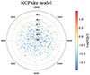 |
Fig. 1. Sky model of the North Celestial Pole at 141 MHz input to the forward simulations. The flux densities are intrinsic and beam-corrected. It is composed of 684 unpolarized point sources with a flat spectrum. The bright radio source at Dec ∼ 86.3° and RA ∼ 2.5 h is 3C 61.1. |
3.1.2. Diffuse Galactic emission model
Models of diffuse Galactic emission at MHz frequencies remain poorly constrained on small spatial and spectral scales, leading to significant model uncertainties. The most comprehensive all-sky map is still the Haslam map at 408 MHz (Haslam et al. 1981, 1982), which has an angular resolution of ∼1°. A commonly used model in the literature is the Global Sky Model (GSM) (de Oliveira-Costa et al. 2008) and its updated version, the improved GSM (Zheng et al. 2017), both of which are based on a principal component analysis and heavily rely on Galactic observations spanning a broad frequency range. However, the GSM is not reliable on finer angular scales. Some lower-frequency measurements of diffuse emission exist from MWA, LWA1, and OVRO-LWA data (Byrne et al. 2022; Dowell et al. 2017; Eastwood et al. 2018) at frequencies below 200 MHz. The 182 MHz diffuse emission map by Byrne et al. (2022) covers angular scales from 1 to 9 degrees but is limited to a single frequency without spectral information. The LWA1 Low Frequency Sky Survey (Dowell et al. 2017) spans 35 MHz to 80 MHz with angular scales of 2°–4.7°. Gehlot et al. (2022) modeled the diffuse Galactic emission at 122 MHz around the NCP with the LOFAR-AARTFAAC system using multiscale CLEAN and shapelet decomposition. While the multiscale CLEAN method is able to model extended emission at intermediate angular scales of ≲2.3°, it is sub-optimal for modeling larger scales of the order of a few degrees. The shapelet decomposition on the other hand is best suited to model larger angular scales.
We found that none of these models were suitable as a model of the diffuse Galactic foregrounds for the desired observational field, angular resolution and spectral information. We therefore describe the foregrounds as a Gaussian random field generated from an angular covariance function informed by the above-mentioned NCP data obtained with LOFAR-AARTFAAC. Spatially, the Gaussian random field does not resemble our Galaxy, but it provides a good approximation, as its underlying statistic, the angular correlation function, is similar. Nevertheless, for the purpose of studying the effects of unmodeled diffuse Galactic emission on calibration, this approach is sufficient
Our model of the diffuse Galactic synchrotron emission is based on Santos et al. (2005) and is described by an angular power spectrum as a function of angular scale, l, and frequency, ν, of the form,
 (1)
(1)
where α is the power law index for the spatial spectrum, β is the power law index for the frequency spectrum, and ζ describes frequency correlation. For this work, we only considered unpolarized Galactic synchrotron emission. The parameters for this model were informed by Gehlot et al. (2022) and Bernardi et al. (2009). Gehlot et al. (2022) measured the Galactic radio emission at 122 MHz around the NCP with LOFAR-AARTFAAC at angular scales 20 ≲ l ≲ 200 and found a brightness temperature variance of Δl = 1802 = (145.64 ± 13.61)K2 on angular scales of 1 degree. Using the relation Δl2 ≡ l(l + 1)Cl/2π, we defined the amplitude, A, of the angular power spectrum model (Equation 1) as the brightness temperature variance at l0 = 180 and ν0 = 122 MHz. We found A = 0.0028 K2. The power-law index parameter for the spatial spectrum α is guided by measurements of the NCP with LOFAR-AARTFAAC by Gehlot et al. (2022), who found α = 2.0 for l ≲ 200 and measurements of the low Galactic latitude Fan region with the Westerbork synthesis radio telescope (Bernardi et al. 2009) who found α = 2.2 for l ≲ 900. We adopted α = 2.2 for our model because the spatial spectrum in Bernardi et al. (2009) was fitted over a broader multipole range. The detection of diffuse structure beyond l ∼ 900 is limited by residual point sources, but we assumed the power-law scaling holds to higher multipoles for modeling purposes. For the spectral index, we adopted β = 2.55 for frequencies between 100 MHz to 200 MHz and high Galactic latitudes (Rogers & Bowman 2008). The spectral index of the angular power spectrum of the Galactic radio diffuse synchrotron emission typically steepens with increasing frequency corresponding to a softer electron spectrum (de Oliveira-Costa et al. 2008). For the Galactic synchrotron emission, we adopted a frequency correlation parameter ζ = 4, following Santos et al. (2005). We summarize the model parameters of the angular power spectrum in Table 1.
Parameters for our diffuse Galactic emission angular power spectrum model.
We simulated a full-sky Gaussian foreground healpix map modeled by the angular covariance defined in Equation (1), using the model parameters from Table 1 and the Python package cora16. This simulation spans a frequency range of 146.9 MHz to 159.6 MHz, corresponding to a redshift range of z ∼ 8.0 − 8.7, one of the redshift bins analyzed in the LOFAR-EoR NCP data processing. We chose healpix NSIDE parameter of 2048, corresponding to an angular resolution of 1.7 arcmin. A 10° ×10° FoV was projected onto a 2D Cartesian grid with 2 arcmin resolution to eliminate nearest-neighbor interpolation effects (see Figure 2). To avoid Gibbs ringing, the mean of each 2D image was subtracted. Finally, we converted the brightness temperature, T, to the flux density in units of Jy/pixel, as required for predicting visibilities with WSCLEAN, using the Rayleigh-Jeans law,
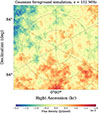 |
Fig. 2. Diffuse Galactic emission is modeled as a Gaussian random field with an angular covariance informed by measurements of the NCP at 122 MHz with LOFAR-AARTFAAC data and the Fan Region at 150 MHz with the Westerbork telescope. |
 (2)
(2)
where kB is the Boltzmann constant, Ω is the image pixel area, and the flux density S is expressed in units of  . The 2D images were then placed into fits files using the header information from images created from predicted visibilities of the NCP model, which includes information such as the pointing of the telescopes, the observing frequency, and the point spread function.
3.1.3. Prediction of the beam
The prediction of the LOFAR-HBA beam was enabled using SAGECAL-CO during visibility simulation. To achieve a realistic representation of LOFAR-HBA observations of the sky, both the element beam and array factor were included. The element beam is the response of a single dipole antenna within a tile, with an instantaneous FoV of half the sky. The array factor models phasing up the 16 dual-polarization antennae to a tile beam, and further phasing of tiles into a station beam. The simulation also incorporated the effects of defunct and switched-off tiles, as recorded in the measurement set, to accurately represent the distorted station beam. The same beam model was applied during data analysis, ensuring consistency between the simulated visibilities and the calibration and imaging steps, thereby avoiding any discrepancies due to mismatched beam assumptions.
3.1.4. Prediction of visibilities
The prediction of visibilities for the point-source model was implemented with SAGECAL-CO, which calculates the radio interferometer measurement equation (RIME) (Hamaker et al. 1996; Smirnov 2011) for every single point source, k, provided in the sky model file,
 (3)
(3)
The visibility matrix, Vij(t, ν), is a 2 × 2 complex matrix that represents the full-polarization cross-correlations between the signals from two beam-formed stations i and j, as a function of time, t, and frequency, ν. Here, Ji is a 2 × 2 complex matrix called the Jones matrix describing the instrumental response of a radio interferometer to the incoming electric field; Cij; k is the coherency matrix for each sky model component, k, measured by the baseline, ij. It essentially describes the flux density of a compact source component in terms of the Stokes parameters I, Q, U, and V.
Visibilities were predicted using the uvw-coordinates and local sidereal time (LST) ranges from the LOFAR-HBA EoR observation targeting the NCP with a phase center at Dec = 90.0°. We simulated a total bandwidth of 12.7 MHz between observing frequencies 146.9 MHz to 159.6 MHz corresponding to the lowest redshift bin using all core and remote stations. The measurement set from the real LOFAR observation and used as a template in this study provides all essential information about the interferometric array. This includes the details of inactive tiles per station and allows for a realistic simulation of the time-dependent station beam. To reduce computation time, we limited the dataset size by selecting a 4-hour observation window, while maintaining good uv coverage. For the same reason, we adopted a time resolution of 10 s and a frequency resolution of 195 kHz. A summary of properties of the simulated observational dataset is presented in Table 2.
Properties of the simulated dataset based on real LOFAR-HBA observations of the NCP.
The simulation of the diffuse emission was performed with the image-domain gridder (van der Tol et al. 2018; Veenboer 2021) of WSCLEAN, which enables the application of both the array factor and the primary beam. A 300 × 300 pixel image corresponds to simulating ∼105 components with the standard RIME equation, which is computationally infeasible with our current computational resources. Gridding involves applying a fast Fourier transform to the image, where instead of calculating the transform at every possible point in the uv plane, it can be computed only at regularly spaced grid points. This approach significantly speeds up the prediction of visibilities for diffuse emission, compared to using a direct Fourier transform.
3.1.5. Simulation of thermal noise
Next, we simulated thermal noise according to the radiometer equation,
 (4)
(4)
The system equivalent flux density (SEFD) is a measure of the sensitivity of a radio telescope system, Δt is the integration time and Δν is the spectral resolution. The SEFD was measured for each station as a function of frequency and tabulated (van Haarlem et al. 2013). Thermal noise was generated by drawing from a Gaussian distribution given by σ and a mean of zero and added to the visibility matrix using the LOFAR Simulation Tool losito.
3.2. LOFAR-EoR data processing pipeline
In this section, we outline the key steps of the LOFAR-EoR data processing pipeline for the NCP deep field (Mertens et al. 2020) relevant to this study. These include DI gain calibration of visibilities using SAGECAL-CO, imaging the gain-corrected gridded visibilities with WSCLEAN, and power spectrum estimation using pspipe.
3.2.1. Direction-independent gain calibration
The DI gain calibration refers to the correction of complex gain variations that are common across the entire FoV of the radio interferometer and therefore do not vary with direction on the sky. Key sources of direction-independent errors include: (1) complex gain variations in the analog signal chain due to temperature fluctuations, cable reflections, etc.; (2) clock and time synchronization errors; (3) ionospheric effects on short time scales; and (4) differences between the sky model and the true sky, along with beam errors, which can lead to inaccuracies in calibration, contributing to an overall mismatch between the expected and the observed sky. The DI gain calibration is aimed at correcting these types of errors by using a catalog of bright sources using the sky model. The resulting gain solutions can then be applied uniformly across the entire FoV, correcting for the average flux density of the field.
Since the brightest source in the NCP field, 3C 61.1, is close to the first null of the primary beam of the station, DI gain calibration for observational data is actually performed in two directions to separate the strong DD effects for this source. For our forward simulations, we decided to stick to calibrating to a single direction, since our simulated visibilities are not corrupted by any gain errors other than the ones introduced by calibrating with a sky model omitting diffuse Galactic emission. We also found no significant difference in the gain solutions when calibrating in one direction compared to two directions in our simulations.
The DI gain calibration was performed using SAGECAL-CO, which employs consensus optimization (Boyd et al. 2011) to iteratively adjust station gain solutions, driving them towards spectrally smooth functions that are also optimized. The key idea behind consensus optimization is to have different agents work on separate parts of the problem while ensuring that their solutions converge to a common consensus. At each iteration, solutions that deviate from a frequency-smooth prior are penalized by a regularization term, the strength of which is determined by a parameter ρ, which is then updated. Eventually this process should converge to the prior. For a more detailed and mathematical description of the SAGECAL-CO algorithm, we refer the readers to Yatawatta (2015, 2016).
Improving DI gain calibration has been a major focus of reprocessing the LOFAR NCP data over the past year. This was accomplished by employing a two-step approach to minimize the number of free parameters in the DI gain calibration, leading to a reduction in gain errors on small spectral scales that could otherwise affect or mimic the 21 cm signal. Delay spectra of the normalized gain solutions showed a decrease in power by two to three orders of magnitude when using the two-step approach with regularized gains, compared to the one-step approach with unregularized gains (Mertens et al. 2025). For our simulations, we followed the same two-step DI gain calibration scheme:
-
Step 1: Correction of smooth spectral and fast temporal gain variations;
-
Step 2: Correction of fast varying bandpass and slow temporal gain variations.
For the first DI step, we used a third-order Bernstein polynomial over the 12.7 MHz bandwidth, consistent with the analysis of LOFAR-EoR NCP data (Mertens et al. 2020). The optimal regularization parameter was found by running DI gain calibration on forward simulated noisy visibility data as a function of regularization parameter with a fixed number of iterations and quantifying the variance of the sub-band differenced gain solutions. A clear minimum was found at ρ = 200, which verifies the results by Yatawatta (2016) and Mertens et al. (2020). Low or no regularization will over-fit the data, resulting in signal suppression on the smallest baselines where we are most sensitive to the 21 cm signal (Patil et al. 2017; Mevius et al. 2022). Calibration was performed on a spectral and time solution interval of 195.3 kHz (one sub-band) and 30 s, respectively. We used a total of 40 ADMM (Alternating Direction Method of Multipliers (Boyd et al. 2011)) iterations during the optimization, which was found to be sufficient to achieve the required convergence (Mevius et al. 2022). Baselines between 50 − 5000 λ were used.
In the second DI gain calibration step, we solved for the fast frequency-varying bandpass response of the stations, which in real data, is caused by filter amplifiers in the signal chain and coaxial cable reflections between receivers and tiles, but does not vary with time. These effects, however, are not present in the simulated data. Nonetheless, for consistency with real data processing, we apply the same DI gain calibration procedure to the simulations. Unregularized DI gain solutions were found on a per-frequency-subband basis. We set the time solution interval to 4 h, which corresponds to the duration of the simulated observation and is also the maximum amount of data that can be processed by a single NVIDEA K40 GPU on the supercluster DAWN, the high-performance computing (HPC) system currently used for analysis of real LOFAR-EoR observations and simulations. Again, baselines between 50 − 5000 λ were used. The gain solutions from both DI steps were applied sequentially to the simulated visibilities for the entire field of view.
3.2.2. Imaging
The gain-corrected visibilities were gridded and each sub-band was imaged independently using WSCLEAN (Offringa et al. 2014), creating an (l, m, ν) image cube. We followed the same gridding procedure as in the LOFAR NCP data processing (Mertens et al. 2020) with unit weighting during gridding and a Kaiser-Bessel anti-aliasing filter with a kernel size of 15 pixels, an oversampling factor of 4096 and 32 w-layers. Additionally, we selected baselines between 30 − 250 λ, 0.5 arcmin resolution and 1024 × 1024 pixels. These settings ensured that any systematic effects due to gridding are subdominant to the expected 21 cm signal and thermal noise (see Figure 8 in Offringa et al. 2019a and Figure 5 in Offringa et al. 2019b).
Stokes I and V images, in units of Jy/PSF, as well as the point-spread function (PSF) maps were created with natural weighting. To estimate the thermal noise variance in the data, images were produced from gridded time-differenced visibilities between even and odd (i.e., alternating) time samples. Different sub-bands were then combined to form image cubes with a FoV of 8.5° ×8.5° and 0.5 arcmin resolution. To ensure that the analysis focused on the most sensitive part of the primary beam (with a full width at half maximum (FWHM) of 4.1° at 150 MHz), image cubes were trimmed using a Tukey spatial filter with a diameter of 4°. This aligns with our approach to real data.
3.2.3. Power spectrum estimation
The power spectrum estimation was performed using the Python package pspipe17 and described in detail by Mertens et al. (2020). The cylindrically averaged power spectrum P(k) as a function of wavenumber, k, is defined as:
 (5)
(5)
where  is the Fourier transform in the frequency directions, ΩPB is the integral of the primary beam gain squared over solid angle, B is the frequency bandwidth and X and Y are conversion factors from angle and frequency to comoving distance. The expectation values indicate averaging over baselines within a (k⊥, k∥) power spectrum bin.
The Fourier modes k⊥ and k∥ are wave numbers in units of inverse comoving distance and given by Morales & Hewitt (2004):
 (6)
(6)
where DM(z) is the transverse co-moving distance, ν21 is the frequency of the hyperfine transition of neutral hydrogen, and H(z) is the Hubble parameter.
4. DI gain calibration errors due to unmodeled diffuse Galactic emission
As described in Section 3.2.1, gain calibration is done using a non-linear optimization method named SAGECAL-CO. Gain solutions are obtained through an iterative process, as the minimization of the Lagrangian lacks a closed-form solution. Consequently, deriving an analytic formalism for gain errors is challenging. While some approaches to linearizing the problem exist in the literature (Grobler et al. 2014; Wijnholds et al. 2016), our focus is on providing a qualitative description of the gain calibration process in the presence of unmodeled Galactic diffuse emission, aiming to build intuition for the reader.
For the purposes of this paper we only consider unpolarized foreground emission, since this is the most dominant component, and set Q, U, V = 0. Furthermore, we assume that unpolarized foreground emission consists of a point source and a Galactic diffuse component, denoted by the coherency matrix CP and CD, respectively. We define the true visibilities as the total foreground emission measured by the interferometer. They represent the ”true” data:
 (7)
(7)
where Ji; k and Jj; k are the true Jones matrices (gains) of stations i and j in direction k, and Nij represents the additive noise. During gain calibration, SAGECAL-CO uses a sky model to compute model visibilities, which are updated at each iteration based on the current gain estimates (Yatawatta 2015). In this study, we assess calibration errors introduced by unmodeled diffuse Galactic emission. To quantify their effect on the gain solutions, we simulate visibilities that include both point sources and diffuse Galactic emission (PSDE), but calibrate them using a point-source-only (PSO) sky model. We refer to this setup as mismatched sky model calibration, since the sky models used in the forward simulation and calibration differ.
Since the goal is to minimize the difference between data and model, some of the power from the diffuse emission will be absorbed into the final gain estimates  . A previous study (Patil et al. 2016) demonstrated that when using all baselines, polarized diffuse emission can be absorbed into the DD gain solutions. This effect occurs because the point spread function (PSF) adapts to compensate for the missing diffuse sky model components, while largely preserving the positions and flux densities of discrete point sources. The DI gain calibration allows us to correct for
  by applying the inverse of the Jones matrix to retrieve the intrinsic flux density of the sky. Due to the omission of diffuse Galactic emission in the calibration sky model, the estimated gains deviate from the true gains, such that
  . The DI gains can be applied directly to the simulated data; hence, the DI-gain calibrated visibilities for every time step, t, and frequency, ν, are
![Mathematical equation: $$ \begin{aligned} \mathbf V _{ij}^{\mathrm{DI-cal} } = \tilde{\mathbf J} _i^{-1} \left[ \mathbf J _i \left( \mathbf C _{ij}^\mathrm{P} + \mathbf C _{ij}^\mathrm{D} \right) \mathbf J _j^{\dagger } + \mathbf N _{ij} \right] \tilde{\mathbf J} _j^{\dagger -1}. \end{aligned} $$](/articles/aa/full_html/2025/12/aa54993-25/aa54993-25-eq13.gif) (8)
(8)
We dropped the direction index, k, since we intended to consider the calibration only in one direction. As mentioned in Section 3.2.1, DI gain calibration is performed in two steps: (1) correcting smooth spectral variations and fast time-varying fluctuations and (2) correcting fast-varying band-pass effects and slow time-varying variations (bandpass calibration). Hence, our gain estimates are a multiplication of the Jones matrices of the two calibration steps:  . All results presented in this paper refer to the combined Jones matrix from steps 1 and 2 of the DI gain calibration.
In order to compare the estimated gains  affected by unmodeled diffuse emission to unaffected gains, we performed a control simulation where visibilities were forward-simulated using only the point-source catalog, hence,
 (9)
(9)
We then performed the DI gain calibration using a PSO sky model. As this scenario assumes perfect knowledge of the sky model and the instrument, except for thermal noise, we refer to it as matched point-source only (PSO) calibration or the ground truth throughout the paper. Under these idealized conditions, the true gains are expected to be close to unity.
5. Results
This section analyzes the effects of DI gain calibration errors due to the missing diffuse Galactic emission model. We first examine the gain solutions themselves, assess the impact of these calibration errors in image space, and evaluate their effect on the 2D cylindrically averaged power spectra in comparison to thermal noise. Ultimately, we assess the extent to which these errors impact the detectability of the cosmological 21 cm signal in the power spectrum.
5.1. Gain solution analysis
There are a few concerns we would like to address, listed below:
-
We consider whether there is a bias in the gain solutions when calibrating with a sky model that is omitting diffuse Galactic emission and the percentage to which they deviate from unity compared to the ground truth.
-
We consider whether the variance in the gain solutions increase when diffuse Galactic emission is unmodeled in the calibration process.
-
We consider whether the fractional change in power in the gain solutions is dependent on baseline length, given that diffuse Galactic emission is mainly detected with shorter baselines.
As described in Section 3.2.1, for the DI gain calibration, we used baselines in the range of 50 − 5000 λ, a frequency regularization parameter of ρ = 200 and a time solution interval of 30 s. Since the baseline cut is in units of λ, some baselines including LOFAR remote stations have frequency channels for which the corresponding (u, v)-positions fall inside and outside the 5000 λ limit. The gain solutions for these stations were obtained from a subset of the correlation products and are therefore less constrained and noisier. In the future, LOFAR data processing will move to a baseline cut in units of meters.
In Figure 3, we show the normalized histograms of gain amplitude solutions at 152 MHz for all stations and times, representing empirical probability density functions (PDFs). This frequency is representative for mid-band frequencies, whereas frequencies at the edge of the bandwidth generally have wider distributions due to the functional shape of the third-order Bernstein polynomial. The gains were referenced to the Jones matrix of the core station CS001HBA1 by multiplying the gain matrices with the inverse gain matrix of CS001HBA1. Each subplot represents the amplitude of the complex gain solutions for an element of the Jones matrix. J00 represents the response of the x-polarization feed to the x-component of the electric field, Ex, J01 represents the response of the x-polarization feed to the y-component of the electric field, Ey, and so forth. The sky model was forward simulated as unpolarized, so the off-diagonal elements are expected to be zero, except for instrumental polarization leakage caused by non-orthogonal feeds. Blue shows the gain amplitude solutions for the ground truth case, obtained by forward-simulating and calibrating with a PSO sky model. Orange indicates the gain amplitude solutions obtained from a mismatched sky model calibration, where visibilities were forward-predicted using both point sources and diffuse emission (see Equation 7), but calibration was performed using only the PSO catalog. Overlaid are the Rice distribution fits for both calibration scenarios, obtained via MCMC sampling of the posterior distribution for the noncentrality parameter, as well as the location and scale parameters. The Rice distribution fit for J00 reveals that the noncentrality parameter decreases from 9.0 in the matched PSO sky model calibration to about 8.1 in the mismatched case, indicating reduced signal coherence when diffuse Galactic emission is omitted. Similarly, the scale parameter σ increases from roughly 0.0048 to 0.0076, reflecting greater scatter in the gain amplitude solutions under the mismatched sky model calibration. The location parameter μ shows a slight decrease from about 0.96 to 0.94, suggesting a minor systematic shift in the gain amplitude distributions. We found similar results for J11.
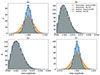 |
Fig. 3. Normalized histograms of the gain amplitudes at 152 MHz for all stations and time solutions. Solid lines show Rice distribution fits for each calibration scenario. Each panel represents a matrix element of the Jones matrix. The gains are referenced to the core station CS001HBA1 by multiplying them with the inverse gain matrix of CS001HBA1. The blue histogram shows the empirical PDF of gain amplitude solutions for the ground-truth case, obtained by forward-simulating and calibrating with a PSO sky model. The orange histogram shows the empirical PDF for gain solutions from simulations using a PSDE sky model but calibrated with a PSO model, thus omitting diffuse Galactic emission during the DI gain calibration, as described in the text. |
To summarize, the standard deviation on the diagonal of the Jones matrix increases by approximately a factor of two when using a mismatched sky model calibration. This means that, on average, the power of the diffuse emission is absorbed or redistributed into the gain solutions, making them noisier when calibrating with a PSO sky model and introducing a systematic error. Note that this normalized histogram is over all stations and time samples and does not highlight any baseline dependent effects.
In Figure 4, we show the effect of neglecting the Galactic diffuse emission in the DI gain calibration process on the gain visibility matrix as a function of baseline length. The top panel shows the baseline lengths corresponding to the upper triangle of the Nstation2 visibility matrix. The first 12 core stations constitute the heart of the core, named the “Superterp” (ST), and reside on a 320 m diameter island. They create the shortest baselines of the LOFAR interferometer most sensitive to diffuse emission, apart from the intra-core station baselines (first off-diagonal matrix elements). The remaining 36 core stations (CS) form baselines extending up to approximately 2000 λ, followed by 14 remote stations (RS). While CS and RS are often distinguished by baseline length, a more critical distinction for calibration is that core stations share a centralized clock enabling coherent beamforming, whereas remote stations use independent, GPS-disciplined rubidium clocks and therefore require explicit correction for clock offsets and drift, particularly important when working with real observational data. Furthermore, to approximate the beam characteristics of core stations, LOFAR remote stations deactivate 24 of their 48 tiles. The resulting beam pattern still differs slightly from that of a true core station due to residual electromagnetic coupling between the active inner tiles and the powered-off outer tiles (Mertens et al. 2025).
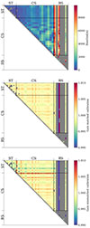 |
Fig. 4. Top: Baseline lengths for the upper triangle of the visibility matrix. ST denotes Superterp core stations, CS core stations, and RS remote stations; these labels act as proxies for baseline lengths. Baselines < 50 λ and > 5000 λ at an observing frequency of 152 MHz are masked in grey. Middle: Absolute value of the time-averaged gain products for the upper triangle of the visibility matrix in the ground truth scenario. Bottom: Same as the middle panel, but forward-simulating with a PSDE sky model and calibrating with a PSO sky model, thereby neglecting diffuse Galactic emission during DI gain calibration. |
Baselines < 50 λ and > 5000 λ at frequency 152 MHz are masked in grey since they are not considered during DI gain calibration. In the middle panel we show the amplitude of the gain visibility matrix averaged over time solutions for the ground truth case, obtained by forward-simulating and calibrating with a PSO sky model for frequency 152 MHz. We created an upper triangle gain visibility matrix by multiplying the station gain Ji with the corresponding Hermitian Jj† for baseline ij and computing the absolute value of the first element of the Jones matrix: |JiJj†|00. Variations in the gain products are of the order of ∼0.5%, likely due to thermal noise variations in the visibilities. RS with baselines near the 5000 λ cut have less constrained gain solutions due to missing data, resulting in high noise levels. As a result, their gains deviate by more than 1% from unity. The bottom panel indicates |JiJj†|00 when forward-simulating a PSDE sky model and calibrating with a PSO sky model, which omits the diffuse Galactic emission in the calibration process. Variations increase from 0.5% to 1% in specific gain visibilities involving the Superterp and nearby core stations, indicating that diffuse Galactic emission is absorbed into the gain solutions as a function of baseline length, with shorter baselines showing a stronger effect.
5.2. Analysis in image space
To show the effect of calibration errors due to the missing diffuse Galactic emission component in image space, we created images from the true (before the DI gain calibration) and DI gain-calibrated visibilities with a minimum and maximum baseline distance of 50 − 250 λ. These are similar baselines that are used in LOFAR’s EoR 21 cm power spectrum analysis. All images were created using WSCLEAN with an angular resolution of 2 arcmin, 10° ×10° FoV and uniform weighting. The units are in Jy/PSF. Figure 5 shows the full sky model (point sources and diffuse emission) in the left panel and the diffuse emission (as seen by the LOFAR-HBA instrument) in the middle panel. The diffuse emission is at least an order of magnitude fainter than the point sources for baselines 50 − 250λ. The imprint of the primary beam is clearly visible, suppressing structures beyond the FWHM of ∼4°. The right panel shows the residual emission by differencing the image of the DI gain-calibrated sky from the true sky. We see an RMS of ∼6 × 10⁻³ Jy/PSF, which is an order of magnitude lower than the RMS from the modeled diffuse emission. For shorter baselines, the gain errors are between 0.5%−1%, which corresponds to flux density fluctuations of ∼5 × 10⁻³ Jy to 1 × 10⁻² Jy for a 1 Jy source; this is similar to the level of residual emission we observe in the right panel of Figure 5.
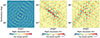 |
Fig. 5. Left panel: Image of the true sky including point sources and diffuse emission. All images are created at frequency 152 MHz with a minimum and maximum baseline distance of 50λ – 250λ. Middle panel: Diffuse emission with a 4 h track point spread function of LOFAR-HBA applied. Right panel: Residual emission is obtained by subtracting the image created prior to the DI gain calibration from the one created afterward. |
To further illustrate the impact of diffuse Galactic emission during DI gain calibration, we compare residual emission in image space between two scenarios: (1) matched PSO calibration, where both the simulated sky and calibration model contain only point sources (left panel of Figure A.1 in Appendix A); and (2) mismatched sky model calibration, where the simulated sky includes both point sources and diffuse emission (PSDE), but calibration is performed using only the PSO model (right panel of Figure A.1 in Appendix A, identical to the right panel of Figure 5). In both cases, the residual emission is computed by subtracting the DI gain-calibrated sky from the true sky. This comparison clearly shows that diffuse Galactic emission is absorbed into the DI gain solutions for mismatched sky model calibration and appears as residual emission in image space. Since the inverse of the gains is applied directly to the visibilities this leads to a propagation of these errors to subsequent data analysis steps such as power spectrum estimation, which is discussed next.
5.3. Fiducial power spectra
Figure 6 shows the fiducial power spectra of the different components of our simulated data, namely the point sources (left panel), the diffuse Galactic emission (middle panel) and the thermal noise (right panel). Spectrally smooth foregrounds dominate the lowest k∥-bins. The point source power spectrum shows higher power at larger k⊥ because the power spectrum of point sources remains flat with respect to angular scale (which is inversely proportional to baseline length), whereas the power spectrum of diffuse emission decreases as the angular scale becomes smaller. The spread of foreground power into higher k∥-bins at increasing k⊥, known as the “foreground wedge”, is caused by the instrument’s chromaticity. The noise power spectrum is flat as a function of k∥ for fixed k⊥. Power spectrum bins associated with uv-bins that contain less visibility data exhibit higher noise power.
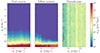 |
Fig. 6. Fiducial 2D cylindrically averaged power spectra of simulated data from a point source model (left panel), from a diffuse Galactic emission model (middle panel) and from thermal noise (right panel). |
5.4. Matched point-source-only calibration
In a control simulation, we generated simulated data that included only a point-source sky, without any diffuse Galactic emission. We added thermal noise to the simulation, creating ten different versions of this data, each with a unique realization of thermal noise drawn from the same distribution. Then, we calibrated these visibilities using a model that matched the point-source sky (i.e., the sky model used for calibration was complete and accurate). This process produced ten correctly calibrated power spectra, each representing the simulated data under a different thermal noise realization.
In this setup, any bias or variance in the power spectrum arises solely from thermal noise variations. To estimate the systematic bias, bsys, we calculated the mean residuals of the ten estimated power spectra relative to the fiducial true power spectrum using the power spectrum estimator discussed in Section 3.2.3:
 (10)
(10)
Here, Pi represents the calibrated power spectrum, while ⟨Ptrue⟩ represents the fiducial true power spectrum, derived by averaging ten power spectra generated from true visibilities  under variation of thermal noise. The angle brackets ⟨...⟩ denote ensemble averages over the ten realizations. We will define several configurations for our simulations in this study:
-
Setup 1 is the ground truth and control simulation. ⟨ΔPNiDI − cal⟩ is the estimated expectation value of the power spectrum residuals, when DI gain calibration is performed with a matched sky model and the thermal noise realization is varied. The fiducial power spectrum ⟨Ptrue⟩=⟨PP + PNi⟩ is the ensemble average of power spectra generated from true visibilities with different thermal noise realizations.
Since thermal noise and solver noise18 is incoherent between realizations, we expect ⟨ΔPNiDI − cal⟩ to approach zero as the number of realizations increases, except for in the lowest k∥-bins, where the foregrounds are located. We show the power spectrum residuals of setup 1 as a fraction of the expected thermal noise in the left panel of Figure 7. It should be noted, that even when we calibrate with a matched sky model, there is a systematic bias in the lowest k∥-bins simply due to thermal noise variations. Thermal noise introduces slight inaccuracies in gain calibration, subsequently modulating the foregrounds. A key question arises: if the impact on the gains is random, why does it still lead to a systematic offset that results in an overall increase in power in the lower k∥-bins? When constructing the power spectrum, visibilities within a single uv cell are averaged and then squared. DI gain-corrected visibilities are modified by two estimated Jones matrices,  and
and  , following Equation (8). If both
  and
and  contain Gaussian noise, the expectation value of Equation (8) becomes biased, leading to an excess in power. The bias is confined to the lowest k∥-bin, due to the frequency-smooth constraint during the DI gain calibration.
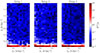 |
Fig. 7. Systematic bias as a fraction of the thermal noise for a simulation with matched sky model DI gain calibration (forward simulation and calibration with a PSO sky model) in the left panel (setup 1) and with a mismatched sky model DI gain calibration (forward-simulation with a PSDE sky model and calibration with a PSO sky model, which is missing the diffuse Galactic foreground component), in the middle panel and right panel (setups 2 and 3). The systematic bias is estimated from ten power spectra under variation of thermal noise (setup 1), diffuse foregrounds (setup 2), thermal noise and foregrounds (setup 3), respectively, in the visibility simulation. Blue regions indicate that the systematic bias is below the estimated thermal noise and red regions above. |
5.5. Mismatched sky model calibration
In this section, we assess the impact of unmodeled diffuse Galactic emission during the DI gain calibration in the simulation. Therefore, we forward-simulated a PSDE sky model to obtain visibilities, but then used a DI gain-calibration on the data with a PSO sky model. This produced a mismatch between the forward simulation and the calibration process. Next, we evaluated the systematic power spectrum bias, bsys, resulting from calibration errors due to the omission of diffuse Galactic emission.
To achieve this, we generated ten power spectra from DI gain-calibrated visibilities ( ), where each power spectrum corresponds to a different Gaussian realization of the diffuse foregrounds. The point-source sky and noise realization were held constant to isolate the calibration errors caused by unmodeled diffuse Galactic emission from other sources of variation. This setup ensures that we can attribute any residual power spectrum bias to the errors introduced by the mismatched sky model with a statistical sample variance of 10%.
However, to accurately disentangle the bias caused by calibration errors from the effects of thermal noise variations, we performed an additional simulation. In this extended setup, we introduced variations in both Gaussian foregrounds and thermal noise. This allows us to determine how much of the observed bias arises from thermal noise fluctuations versus calibration errors due to the omission of Galactic diffuse emission during the DI gain calibration.
The systematic power spectrum bias for these two setups is again estimated by calculating the mean residuals from the fiducial true power spectrum, according to the Equation (10). Pi is a single estimated power spectrum calculated from miscalibrated visibilities. The two setups are:
-
Setup 2: ⟨ΔPDiDI − cal⟩ is the expectation value of power spectrum residuals, when the DI gain calibration is performed with a mismatched sky model ⟨ΔPDiDI − cal⟩ under different realizations of diffuse foregrounds Di. The fiducial power spectrum ⟨Ptrue⟩=⟨PP + PDi + PN⟩ is the ensemble average of power spectra generated from true visibilities
 under variation of diffuse foregrounds.
 -
Setup 3: ⟨ΔPDi, NiDI − cal⟩ is the expectation value of power spectrum residuals under different realizations of both the diffuse foregrounds and thermal noise, when the DI gain calibration is performed with a mismatched sky model. The fiducial power spectrum ⟨Ptrue⟩=⟨PP + PDi + PNi⟩ is the ensemble average of power spectra generated from true visibilities with different realizations of diffuse foregrounds and thermal noise.
The results of these three setups are shown in Figure 7. The systematic bias, as defined in Equation (10), is expressed as a fraction of the thermal noise power for 4 hours of observations with LOFAR-HBA observations. This represents the average 2D cylindrical power spectrum of Stokes V when the thermal noise realization is varied in visibility space. The systematic bias ranges from 10−3 (blue regions) to 103 (red regions) in the graphs. Blue regions represent power spectrum bins in which the systematic error due to DI gain calibration errors is subdominant to the thermal noise after 4 hours of observations, whereas red regions represent bins in which the systematic error dominates over the thermal noise. Calibrating with a mismatched sky model that is omitting the diffuse Galactic emission (setups 2 and 3), increases the systematic bias by approximately one order of magnitude (see also Figure 8) compared to matched PSO sky model calibration (setup 1), although the systematic bias is mostly confined to k‖ < 0.1 h Mpc−1. Residual foregrounds, which dominate in regions k‖ < 0.2 h Mpc−1, can be removed using GPR (Mertens et al. 2018, 2020, 2024), provided they are coherent between observations and the excess power exhibits a frequency-frequency coherency scale similar to that of the foregrounds. The coherency between pairs of 4-hour observations will be analyzed in the next section.
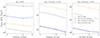 |
Fig. 8. Average systematic bias, the expected thermal noise and the error on the thermal noise as a function of observation time for three different regions in the 2D power spectrum space: The foreground dominated region in panel 1 (k∥-bins < 0.2 h Mpc−1), the short baseline region, where diffuse Galactic emission is prominent in panel 2 (k∥-bins > 0.2 h Mpc−1 and k⊥-bins < 0.1 h Mpc−1) and the noise dominated region in panel 3 (k∥-bins > 0.2 h Mpc−1 and k⊥-bins > 0.1 h Mpc−1). In orange we show the expected thermal noise, in dashed black the error on the thermal noise as a function of integration time and in blue and purple the systematic bias for matched PSO and mismatched sky model calibration, respectively. |
5.6. Coherence of DI gain calibration errors
To better understand whether the excess power from DI gain calibration errors is correlated between nightly observations, we conduct two tests. First, we examine whether the systematic bias integrates down or not as integration time increases. Second, we evaluate the cross-coherency between 4-hour observations taken at different local sidereal times.
5.6.1. Combining data sets
In this section, we present the power spectra obtained by combining three observations taken at different local sidereal times (LST), totaling 12 hours of simulated data. Unlike repeated observations of the same LST with different noise or foreground realizations (Section 5.4 and 5.5), these three observations are spaced 4 hours in LST apart to better reflect realistic observing conditions for a symmetric array such as LOFAR. It is necessary to combine observations to reduce the thermal noise level and to determine if the systematic bias due to DI gain calibration errors remains or is reduced when combining observations from different LST intervals. It is expected that a total of about 1000 hours of LOFAR-HBA observation on a deep field is required for a statistical detection of the 21 cm signal from the EoR (Mertens et al. 2020). These LST intervals account for changes in the PSF over time, with the specifications of the simulated datasets listed in Table 2.
We used inverse variance weighting to optimally average the datasets in visibility space, ensuring an accurate combination of data from different observations for power spectrum estimation. Observation-to-observation variations in noise levels were addressed by using Stokes-V sub-band difference noise estimates, which were combined with weights based on the (u, v) density of the gridded visibilities. The methodology for estimating these weights is described in detail in Section 3.2.3 of Mertens et al. (2020).
To determine the systematic bias, we created a stack of observations both before and after the DI gain calibration. Since our simulations are only 4 hours long, some uv cells contain fewer visibilities. To mitigate this issue, we filtered visibilities with a minimum weight of 100, resulting in gaps in the uv coverage and causing thermal noise to integrate down more slowly in certain regions of power spectrum space when combining observations from different LSTs. The pre-calibration stack serves as our fiducial power spectrum, Ptrue, while the post-calibration stack represents the measured power spectrum with the DI gain calibration errors embedded. The systematic bias for stacks of 1, 2, and 3 observations with different LST ranges, expressed as a fraction of the thermal noise, is shown in Figure B.1 with matched PSO sky model calibration, and in Figure B.2 with mismatched sky model calibration, which omits the diffuse Galactic emission component. These are detailed in the Appendix B. From these, we observe that the systematic bias, for both the matched and mismatched sky model calibration cases, does not clearly decrease with increasing observation time. This suggests that DI gain calibration errors in the foreground dominated region k∥-bins < 0.2 h Mpc−1 are coherent, while thermal noise, which dominates in k∥-bins > 0.2 h Mpc−1, is incoherent and decreases with longer integration times.
To better understand the magnitude of the bias compared to thermal noise and to determine whether it integrates down, we divided the (k⊥, k∥)-space into three regions: the foreground dominated region for k∥-bins < 0.2 h Mpc−1, and two EoR-window regions distinguishing between the shorter baselines (|u|< 100; roughly the LOFAR ‘superterp’ region) with k∥-bins > 0.2 h Mpc−1 and k⊥-bins < 0.1 h Mpc−1 and the longer baselines with k∥-bins > 0.2 h Mpc−1 and k⊥-bins > 0.1 h Mpc−1. The region where |u|< 100, corresponds to prominent diffuse Galactic emission; however, for |u|> 100, noise becomes dominant. We averaged the systematic bias (as defined in Equation (10)) and the thermal noise over power spectrum bins for these three regions and plotted them as a function of number of observations, which corresponds to observation time, on a log-log plot in Figure 8.
In the left panel of Figure 8, which represents the foreground dominated region for k∥-bins < 0.2 h Mpc−1, we clearly observe that the thermal noise decreases with integration time, while the systematic bias is above thermal noise and remains approximately constant. Even though the bias is much higher than thermal noise in the foreground dominated region, GPR is able to remove these signals if they are coherent in frequency and observation time. The frequency coherence is ensured by the smooth gain solutions, ensuring no rapidly varying frequency structures.
In the middle panel, we compare the systematic bias and thermal noise for |u|< 100, corresponding to k∥-bins > 0.2 h Mpc−1 and k⊥-bins < 0.1 h Mpc−1. Here, we find that the systematic bias is 1 − 2 orders of magnitude lower than the thermal noise and ∼ one order of magnitude below the error of thermal noise and it is evident that the thermal noise decreases with a similar slope as the bias as a function of integration time (days). There is a slight difference in the bias between calibrating with a matched sky model versus a mismatched one, although these differences are minimal. Based on these these observations we did a linear fit of the bias, thermal noise power and error on the thermal noise versus hours of integration. The slopes were found to be very similar, indicating that the average power spectrum residuals integrate down in a manner similar to thermal noise. The same conclusion applies for the noise dominated region (k∥-bins > 0.2 h Mpc−1 and k⊥-bins > 0.1 h Mpc−1): the slopes of the thermal noise, error on the thermal noise and bias power are almost identical, meaning the average power spectrum residuals in this region also integrate down like thermal noise. The error on the thermal noise is due to sampling variance, which depends on the number of uv cells averaged into a power spectrum bin. Due to different visibility flagging for different LST ranges, the slope of the error on the thermal noise differs between stacking two observations versus three.
To further investigate whether the DI calibration bias continues to decrease with observation time or eventually plateaus, we also conducted a set of simulations using repeated 4-hour observations at the same LST. In this case, both the sky and the PSF remain fixed, and only the thermal noise is different between the observations. Under these conditions, we observe that the systematic bias still decreases, but with a shallower slope than in the case where observations span different LSTs. This implies that time-varying PSFs, resulting from observing at different LSTs, introduce incoherence in the calibration errors due to mode-mixing, thereby helping the bias integrate down more effectively. To quantify the rate of decrease, we performed a linear fit of the bias and thermal noise power as a function of integration time (in hours). We find that the bias becomes equal to the thermal noise level after approximately 90 hours of integration for the matched PSO calibration and after about 40 hours for the mismatched sky model calibration. This illustrates how calibration errors accumulate differently depending on calibration sky model completeness, and how PSF variation can help mitigate their coherence over time. Extrapolating from these results, after stacking 4-hour observations at the same LST, the bias in the short baseline region reaches the thermal noise level after roughly 10 times the length of a single observation. By analogy, for 12-hour observations at the same LST, we expect the bias to decrease at a similar rate per observation, reaching the thermal noise level after roughly 120 hours of total integration time. This extrapolation assumes the bias behavior from 4-hour blocks scales linearly or comparably for longer periods. While plausible, this assumption should be validated with further simulations or data which is beyond the scope of this work.
We conclude this section that even with thermal noise variations and matched PSO sky model calibration a systematic bias is introduced. Thermal noise variations lead to small gain errors, which, when applied to the bright point source model, introduce a power spectrum bias. However, these errors are only significant at k∥-bins < 0.2 h Mpc−1 and could be mitigated by GPR. The same applies to mismatched sky model calibration, where omitting diffuse Galactic emission from the sky model leads to a bias approximately one magnitude higher in the same region.
5.6.2. Coherence across observations
For GPR to effectively remove excess power within the foreground-dominated region, the signal must exhibit a frequency-frequency coherence scale similar to that of the foregrounds and must be coherent across observations (Mertens et al. 2020). We determine the correlation between all pairs of simulated observations by computing the cylindrically-averaged cross-coherence, defined as:
 (11)
(11)
The cross-coherence is a normalized metric ranging from −1 to 1, where −1 indicates strong anti-correlation, 1 indicates strong correlation, and 0 signifies no correlation. If the bias is only partially coherent in either of the two EoR-window regions, it not only averages down more slowly than incoherent thermal noise (as demonstrated in the previous section), but also introduces a bias in the 21 cm signal power spectrum that increases with longer integration times and cannot be mitigated by standard GPR. This is because, in the current NCP pipeline, GPR is applied after combining data from multiple nights, which limits its ability to mitigate a partially coherent bias. We note that applying GPR on a per-night basis may alleviate this and is currently under investigation.
To test for cross-coherence across observations, we use the three simulated observations taken at different LST, and compute the cross-coherence between all pairs of observations in the case of matched PSO sky model calibration and mismatched sky model calibration. We show the average cross-coherence over all observation pairs in Figure C.1 of the Appendix C. When differencing the average cross-coherence from simulated observations DI gain-calibrated with a mismatched sky model from the ones calibrated with a matched PSO sky model, we see up to 10% higher coherence in the average cross-coherence obtained from power spectra calibrated with a mismatched sky model, omitting the diffuse Galactic emission. The difference is specifically noticeable on shorter baselines (|u|< 100 and k⊥ < 0.1 h Mpc−1), pointing to partial coherence due to the missing diffuse Galactic emission, which is distinct from incoherent thermal noise at baselines |u|> 100.
To further compress the information from the cross-coherence between all pairs of observations, we again divide the (k⊥, k∥)-space in a foreground dominated region (k‖ < 0.2 h Mpc−1) and the two EoR-window regions separated by baseline length (k‖ > 0.2 h Mpc−1 and |u|< 100 or |u|> 100) and average over the bins in these three regions. A corner-plot of the correlations between observations for each of the three different regions is presented in Figure 9 in the top panel for matched PSO sky model calibration and in the bottom panel for mismatched sky model calibration. In the foreground region (left panels), the signal is predominantly coherent, whereas the EoR-windows exhibit incoherence on average across observations. The short baseline region (middle panel) displays greater coherence on average compared to the noise-dominated region (right panel), with only minor differences observed between calibrating with a matched sky model and a mismatched one.
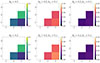 |
Fig. 9. Cross-coherence corner-plot between three different simulated observations covering different local sidereal time (LST) ranges. Top panel: Average cross-coherence when DI gain calibrations are applied to the visibilities with a matched PSO sky model. Bottom panel: Average cross-coherence when DI gain calibrations are applied to the visibilities with an mismatched sky model, which is omitting the diffuse Galactic emission. Three regions of the (k⊥, k∥)-space are analyzed: The foreground region k‖ < 0.2 h Mpc−1 (left panel), and two EoR-windows for k‖ > 0.2 h Mpc−1 and baselines < 100 λ (middle panel), and baselines > 100 λ (right panel). There is on average strong cross-coherence between observations in the foreground region (left panel), whereas weak coherence in the EoR-regions (middle and right panel). There are only minor differences in the average cross-coherence in the EoR-window for baselines < 100 λ, where diffuse Galactic emission is prominent, between calibrating with a matched PSO sky model versus a mismatched one. |
6. Summary and conclusions
We developed a realistic forward simulation pipeline called Simple (SIMulation Pipeline for LOFAR-EoR) using Nextflow, a workflow management tool, to study the impact of diffuse Galactic emission on DI gain calibration for LOFAR-EoR observations. Our DI gain calibration was performed with the non-linear optimization method SAGECAL-CO, which is also typically used for real LOFAR-EoR observations.
Our approach mirrors the two-step DI gain calibration scheme employed in LOFAR-EoR data processing. First, the smooth spectral and rapidly time-varying gain variations were corrected, followed by a band-pass calibration step to address fast band-pass and slow time-varying variations. The gain solutions from both DI steps were combined and applied directly to the simulated visibilities, embedding any DI gain calibration errors in the data and making them challenging to mitigate in subsequent data processing tasks.
Baselines ranging from 50 to 5000 λ were used during the DI gain calibration. Diffuse Galactic emission dominates over confusion noise and could therefore represent the dominant component of the missing sky model on baselines between 50 and 250 λ. This baseline range also corresponds to the range used for EoR 21 cm signal power spectrum analysis. Data were forward-simulated and then calibrated under two scenarios. Scenario 1 represents the ground truth case, obtained by forward-simulating and calibrating with a matched PSO sky model. Scenario 2 was obtained by forward-simulating a PSDE sky model and calibrating with a PSO sky model, thereby omitting diffuse Galactic emission during DI gain calibration. This led to a mismatch between forward-simulation and calibration of the data. The two scenarios enable us to evaluate the impact of unmodeled diffuse Galactic emission relative to a control simulation with a sky model that is complete and accurate. We analyzed the gain solutions, images, and power spectra for the two calibration scenarios, yielding the following results:
-
Gain solution variability: The standard deviation of the histogram of the diagonal gain solutions increases by a factor of ∼2 when calibrating with a mismatched sky model. This indicates that the diffuse emission’s power is redistributed into the gain solutions, making them noisier. Baselines involving the Superterp and nearby core stations (most sensitive to diffuse Galactic emission) show an increase in gain solution variability from 0.5% to 1% with a mismatched sky model calibration.
-
Residual diffuse emission: Residual diffuse Galactic emission appears in image space for baselines between 50 and 250 λ when comparing images before and after DI gain calibration. The RMS of the residual emission is ∼ 6 × 10⁻³ Jy/PSF, roughly an order of magnitude smaller than the original modeled diffuse Galactic emission (∼ 1 × 10⁻² Jy/PSF). Almost no residual emission is observed in the difference images when calibrating with a matched PSO sky model (see Figure A.1).
-
Power spectrum analysis: The systematic bias in power spectrum space, relative to thermal noise, is approximately an order of magnitude higher in the foreground region (k∥ < 0.2 h Mpc−1) for mismatched sky model calibration compared to matched PSO sky model calibration. In the foreground region, the systematic bias does not reduce with integration time (as is the tendency for thermal noise). However, if this bias is coherent across observations (as shown in Figures C.1 and 9), GPR is likely to remove it (Mertens et al. 2018, 2020, 2024) effectively.
-
Integration time requirements: In the EoR-window, for short (|u|< 100) and long baselines (|u|> 100), the bias is 1 − 2 orders of magnitude below the thermal noise and integrates down at the same rate as thermal noise for both DI gain calibration scenarios (matched and mismatched sky model) as a function of observing time. When stacking observations of the same LST range with a fixed PSF, the bias decreases more slowly than thermal noise. Observations with time-varying PSFs cause incoherent DI-gain errors that reduce the bias more efficiently, but after 12 hours, PSF changes no longer help. Based on our analysis in Section 5.6.1, we estimate that the DI gain calibration bias, due to the missing diffuse Galactic component, is expected to approach the level of thermal noise after approximately 120 hours of total integration time; however, this extrapolation remains subject to validation with additional simulations.
-
Coherence analysis: The cross-coherence analysis shows no significant difference in the foreground region (k∥-bins < 0.2 h Mpc−1) between matched and mismatched sky model calibration, indicating that excess power can likely be effectively removed with GPR (Mertens et al. 2018). In the EoR-window for short baselines (|u|< 100), coherence slightly increases with calibration errors from the missing diffuse Galactic emission component compared to matched PSO sky model calibration in some power spectrum bins (see C.1). However, we believe these changes in coherence do not significantly affect the performance of GPR in foreground removal.
Our results indicate that the absence of diffuse Galactic emission in the sky model during calibration is unlikely to be responsible for the excess variance observed in LOFAR’s current 21 cm signal power spectrum upper limits. In real observations, we modeled the diffuse Galactic emission as part of the GPR-based foreground removal step to subtract it from the data. However, this conclusion is based on a simulation that assumed perfect knowledge of the beam. Specifically, the same beam model used during forward simulation was also applied during data analysis, ensuring consistency between the simulated visibilities and the calibration and imaging steps. This approach eliminates any discrepancies arising from mismatched beam assumptions. However, in real-world observations, beam errors can occur, such as tiles being turned off during specific observations. These errors could alter the influence of diffuse Galactic emission on DI gain calibration. Addressing the impact of such beam errors will be the focus of a follow-up study.
Experiment to Detect the Global Epoch of Reionization Signature, https://loco.lab.asu.edu/edges
Shaped Antenna measurement of the background Radio Spectrum, https://wwws.rri.res.in/DISTORTION/saras.html
LOw-Frequency ARray, http://www.lofar.org
Murchison Widefield Array, http://www.mwatelescope.org
Hydrogen Epoch of Reionization Array, http://reionization.org
New Extension in Nanay Upgrading LOFAR, https://nenufar.obs-nancay.fr
Giant Metrewave Radio Telescope, http://gmrt.ncra.tifr.res.in
The LOFAR simulation tool https://github.com/darafferty/losito
Power Spectra Generation pipeline for CD/EoR experiments https://gitlab.com/flomertens/pspipe/
This term refers to the additional noise introduced by the random initialization of parameters in SAGECAL-CO for each calibration run, resulting in slight variations in gain solutions after a finite number of optimization iterations (Mevius et al. 2022).
Acknowledgments
CH, LVEK, SAB, KC, SG and SM acknowledge the financial support from the European Research Council (ERC) under the European Union’s Horizon 2020 research and innovation programme (Grant agreement No. 884760, “CoDEX”). EC would like to acknowledge the support from the Centre for Data Science and Systems Complexity (DSSC), Faculty of Science and Engineering at the University of Groningen, and from the Ministry of Universities and Research (MUR) through the PRIN project ‘Optimal inference from radio images of the epoch of reionization’. FGM acknowledges the financial support of the PSL Fellowship Programme.
References
- Atek, H., Shuntov, M., Furtak, L. J., et al. 2022, MNRAS, 519, 1201 [Google Scholar]
- Barry, N., Hazelton, B., Sullivan, I., Morales, M. F., & Pober, J. C. 2016, MNRAS, 461, 3135 [CrossRef] [Google Scholar]
- Beardsley, A. P., Hazelton, B. J., Sullivan, I. S., et al. 2016, ApJ, 833, 102 [NASA ADS] [CrossRef] [Google Scholar]
- Becker, R. H., Fan, X., White, R. L., et al. 2001, AJ, 122, 2850 [NASA ADS] [CrossRef] [Google Scholar]
- Bernardi, G., de Bruyn, A. G., Brentjens, M. A., et al. 2009, A&A, 500, 965 [NASA ADS] [CrossRef] [EDP Sciences] [Google Scholar]
- Bowman, J. D., Rogers, A. E. E., Monsalve, R. A., Mozdzen, T. J., & Mahesh, N. 2018, Nature, 555, 67 [Google Scholar]
- Boyd, S., Parikh, N., Chu, E., Peleato, B., & Eckstein, J. 2011, Found. Trends. Mach. Learn., 3, 1 [Google Scholar]
- Brackenhoff, S. A., Mevius, M., Koopmans, L. V. E., et al. 2024, MNRAS, 533, 632 [NASA ADS] [CrossRef] [Google Scholar]
- Byrne, R., Morales, M. F., Hazelton, B., et al. 2022, MNRAS, 510, 2011 [Google Scholar]
- Ceccotti, E., Offringa, A. R., Koopmans, L. V. E., et al. 2023, MNRAS, 525, 3946 [NASA ADS] [Google Scholar]
- de Oliveira-Costa, A., Tegmark, M., Gaensler, B. M., et al. 2008, MNRAS, 388, 247 [NASA ADS] [CrossRef] [Google Scholar]
- DeBoer, D. R., Parsons, A. R., Aguirre, J. E., et al. 2017, PASP, 129, 045001 [NASA ADS] [CrossRef] [Google Scholar]
- Donnan, C. T., McLeod, D. J., Dunlop, J. S., et al. 2022, MNRAS, 518, 6011 [NASA ADS] [CrossRef] [Google Scholar]
- Dowell, J., Taylor, G. B., Schinzel, F. K., Kassim, N. E., & Stovall, K. 2017, MNRAS, 469, 4537 [CrossRef] [Google Scholar]
- Eastwood, M. W., Anderson, M. M., Monroe, R. M., et al. 2018, AJ, 156, 32 [NASA ADS] [CrossRef] [Google Scholar]
- Edler, H. W., de Gasperin, F., & Rafferty, D. 2021, A&A, 652, A37 [NASA ADS] [CrossRef] [EDP Sciences] [Google Scholar]
- Ewall-Wice, A., Dillon, J. S., Liu, A., & Hewitt, J. 2017, MNRAS, 470, 1849 [CrossRef] [Google Scholar]
- Finkelstein, S. L., Leung, G. C. K., Bagley, M. B., et al. 2024, ApJ, 969, L2 [NASA ADS] [CrossRef] [Google Scholar]
- Gan, H., Koopmans, L. V. E., Mertens, F. G., et al. 2022, A&A, 663, A9 [NASA ADS] [CrossRef] [EDP Sciences] [Google Scholar]
- Gehlot, B. K., Koopmans, L. V. E., Offringa, A. R., et al. 2022, A&A, 662, A97 [NASA ADS] [CrossRef] [EDP Sciences] [Google Scholar]
- Grobler, T. L., Nunhokee, C. D., Smirnov, O. M., van Zyl, A. J., & de Bruyn, A. G. 2014, MNRAS, 439, 4030 [CrossRef] [Google Scholar]
- Gupta, Y., Ajithkumar, B., Kale, H. S., et al. 2017, Curr. Sci., 113, 707 [NASA ADS] [CrossRef] [Google Scholar]
- Hamaker, J. P., Bregman, J. D., & Sault, R. J. 1996, A&AS, 117, 137 [NASA ADS] [CrossRef] [EDP Sciences] [Google Scholar]
- Harikane, Y., Zhang, Y., Nakajima, K., et al. 2023, ApJ, 959, 39 [NASA ADS] [CrossRef] [Google Scholar]
- Haslam, C. G. T., Klein, U., Salter, C. J., et al. 1981, A&A, 100, 209 [NASA ADS] [Google Scholar]
- Haslam, C. G. T., Salter, C. J., Stoffel, H., & Wilson, W. E. 1982, A&AS, 47, 1 [NASA ADS] [Google Scholar]
- HERA Collaboration (Abdurashidova, Z., et al.) 2023, ApJ, 945, 124 [NASA ADS] [CrossRef] [Google Scholar]
- Hinshaw, G., Larson, D., Komatsu, E., et al. 2013, ApJS, 208, 19 [Google Scholar]
- Jelic, V., Zaroubi, S., Labropoulos, P., et al. 2010, MNRAS, 409, 1647 [CrossRef] [Google Scholar]
- Jordan, C. H., Murray, S., Trott, C. M., et al. 2017, MNRAS, 471, 3974 [NASA ADS] [CrossRef] [Google Scholar]
- Kern, N. S., Parsons, A. R., Dillon, J. S., et al. 2020, ApJ, 888, 70 [NASA ADS] [CrossRef] [Google Scholar]
- Koopmans, L. V. E. 2010, ApJ, 718, 963 [NASA ADS] [CrossRef] [Google Scholar]
- Mertens, F. G., Ghosh, A., & Koopmans, L. V. E. 2018, MNRAS, 478, 3640 [NASA ADS] [Google Scholar]
- Mertens, F. G., Mevius, M., Koopmans, L. V. E., et al. 2020, MNRAS, 493, 1662 [Google Scholar]
- Mertens, F. G., Bobin, J., & Carucci, I. P. 2024, MNRAS, 527, 3517 [Google Scholar]
- Mertens, F. G., Mevius, M., Koopmans, L. V. E., et al. 2025, A&A, 698, A186 [NASA ADS] [CrossRef] [EDP Sciences] [Google Scholar]
- Mevius, M., Mertens, F., Koopmans, L. V. E., et al. 2022, MNRAS, 509, 3693 [Google Scholar]
- Morales, M. F., & Hewitt, J. 2004, ApJ, 615, 7 [NASA ADS] [CrossRef] [Google Scholar]
- Morales, M. F., Hazelton, B., Sullivan, I., & Beardsley, A. 2012, ApJ, 752, 137 [NASA ADS] [CrossRef] [Google Scholar]
- Mouri Sardarabadi, A., & Koopmans, L. V. E. 2019, MNRAS, 483, 5480 [CrossRef] [Google Scholar]
- Offringa, A. R., van de Gronde, J. J., & Roerdink, J. B. T. M. 2012, A&A, 539, A95 [NASA ADS] [CrossRef] [EDP Sciences] [Google Scholar]
- Offringa, A. R., McKinley, B., Hurley-Walker, N., et al. 2014, MNRAS, 444, 606 [Google Scholar]
- Offringa, A. R., Mertens, F., & Koopmans, L. V. E. 2019a, MNRAS, 484, 2866 [CrossRef] [Google Scholar]
- Offringa, A. R., Mertens, F., van der Tol, S., et al. 2019b, A&A, 631, A12 [NASA ADS] [CrossRef] [EDP Sciences] [Google Scholar]
- Ouchi, M., Shimasaku, K., Furusawa, H., et al. 2010, ApJ, 723, 869 [Google Scholar]
- Patil, A. H., Yatawatta, S., Zaroubi, S., et al. 2016, MNRAS, 463, 4317 [NASA ADS] [CrossRef] [Google Scholar]
- Patil, A. H., Yatawatta, S., Koopmans, L. V. E., et al. 2017, ApJ, 838, 65 [NASA ADS] [CrossRef] [Google Scholar]
- Planck Collaboration VI. 2020, A&A, 641, A6 [NASA ADS] [CrossRef] [EDP Sciences] [Google Scholar]
- Rogers, A. E. E., & Bowman, J. D. 2008, AJ, 136, 641 [NASA ADS] [CrossRef] [Google Scholar]
- Santos, M. G., Cooray, A., & Knox, L. 2005, ApJ, 625, 575 [NASA ADS] [CrossRef] [Google Scholar]
- Singh, S., Subrahmanyan, R., Udaya Shankar, N., et al. 2018, ApJ, 858, 54 [Google Scholar]
- Smirnov, O. M. 2011, A&A, 527, A106 [NASA ADS] [CrossRef] [EDP Sciences] [Google Scholar]
- Spinelli, M., Bernardi, G., & Santos, M. G. 2018, MNRAS, 479, 275 [Google Scholar]
- Stark, D. P., Ellis, R. S., Chiu, K., Ouchi, M., & Bunker, A. 2010, MNRAS, 408, 1628 [Google Scholar]
- Tingay, S. J., Goeke, R., Bowman, J. D., et al. 2013, PASA, 30 [Google Scholar]
- Trott, C. M., Jordan, C. H., Midgley, S., et al. 2020, MNRAS, 493, 4711 [NASA ADS] [CrossRef] [Google Scholar]
- van der Tol, S., Veenboer, B., & Offringa, A. R. 2018, A&A, 616, A27 [NASA ADS] [CrossRef] [EDP Sciences] [Google Scholar]
- van Diepen, G., Dijkema, T. J., & Offringa, A. 2018, DPPP: Default Pre-Processing Pipeline, Astrophysics Source Code Library [record ascl:1804.003] [Google Scholar]
- van Haarlem, M. P., Wise, M. W., Gunst, A. W., et al. 2013, A&A, 556, A2 [NASA ADS] [CrossRef] [EDP Sciences] [Google Scholar]
- Vedantham, H. K., & Koopmans, L. V. E. 2016, MNRAS, 458, 3099 [NASA ADS] [CrossRef] [Google Scholar]
- Veenboer, A. 2021, Ph.D. Thesis, Research and Graduation Internal, Vrije Universiteit Amsterdam [Google Scholar]
- Wijnholds, S. J., Grobler, T. L., & Smirnov, O. M. 2016, MNRAS, 457, 2331 [NASA ADS] [CrossRef] [Google Scholar]
- Wilensky, M. J., Morales, M. F., Hazelton, B. J., et al. 2019, PASP, 131, 114507 [NASA ADS] [CrossRef] [Google Scholar]
- Yatawatta, S. 2015, MNRAS, 449, 4506 [Google Scholar]
- Yatawatta, S. 2016, arXiv e-prints [arXiv:1605.09219] [Google Scholar]
- Zarka, P., Denis, L., Tagger, M., et al. 2020, in URSI GASS 2020, Rome, Italy [Google Scholar]
- Zheng, H., Tegmark, M., Dillon, J. S., et al. 2017, MNRAS, 464, 3486 [NASA ADS] [CrossRef] [Google Scholar]
Appendix A: Impact of diffuse Galactic emission on DI-Gain calibration in image space
We generated images of the true sky, which consists of point sources and thermal noise in our ground truth scenario and point sources, diffuse Galactic emission, and thermal noise in the other case. We then created DI-gain calibrated images for both scenarios and subtracted them from their respective true sky images. The Figure A.1 shows the resulting residuals: the left panel corresponds to calibration with a matched PSO sky model, while the right panel corresponds to DI-gain calibration with a mismatched sky model, where diffuse Galactic emission was missing during the calibration process. This highlights how diffuse Galactic emission is absorbed into the DI-gain solutions and appears as residual emission in image space.
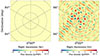 |
Fig. A.1. The left panel shows the residual emission obtained by differencing the DI-gain calibrated sky from the true sky in our ground truth scenario (i.e., when calibrating with a matched PSO sky model). The right panel shows the residual emission obtained when calibrating with a mismatched sky model. |
Appendix B: Systematic bias in stacked power spectra
We combine three simulated observations taken at different local sidereal times separated by 4 hours, by using inverse variance weighting to optimally average the data in visibility space. The systematic bias as a fraction of thermal noise is shown for stacks of 1, 2 and 3 simulated observations in Figure B.1 when DI-gain calibrating visibilities with a matched PSO sky model and in Figure B.2 when DI-gain calibrating with a mismatched sky model. The systematic bias in the foreground region for k‖ < 0.2 h Mpc−1 is at least one magnitude higher when DI-gain calibrating with a mismatched sky model, which is missing the diffuse Galactic emission. As will be shown in the next section C, the bias in the foreground region is highly coherent, therefore our foreground removal method, Gaussian Process Regression (GPR), has proven to be able to remove this excess power.
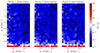 |
Fig. B.1. The systematic bias as a fraction of the thermal noise for matched PSO sky model DI-gain calibration, when the cylindrical Stokes I power spectra are coherently averaged for 1, 2 and 3 observations, respectively. Each observation is 4 hours long and separated by 4 hours in local sidereal time, in order to cover a full day of observation for a symmetric array. |
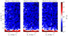 |
Fig. B.2. The systematic bias as a fraction of the thermal noise for mismatched sky model DI-gain calibration, when the cylindrical Stokes I power spectra are coherently averaged for 1, 2 and 3 days, respectively. Each observation is 4 hours long and separated by 4 hours in local sidereal time, in order to cover a full day of observation for a symmetric array. |
Appendix C: Average cross-coherence
The average cross-coherence is calculated by computing the cross-coherence, as defined by Equation 11, for all pairs of observations and then averaging the results. The left panel of figure C.1 shows the average cross-coherence of 2D power spectra derived from visibilities DI-gain calibrated using a matched PSO sky model. The middle panel presents the same analysis for visibilities DI-gain calibrated with an mismatched sky model, which omits the diffuse Galactic emission component. The power spectrum bins in the lowest k∥-bin show high coherence due to the presence of foregrounds. Additionally, regions at low k⊥, which correspond to power spectrum bins associated with uv-cells containing fewer visibilities, also show increased coherence. At first glance, there appears to be no significant difference between the two. However, a comparison of the average cross-coherence between the middle panel (mismatched sky model DI-gain calibration) and the left panel (matched PSO sky model DI-gain calibration) reveals that certain power spectrum bins associated with short baselines exhibit higher coherence when calibrated with the mismatched sky model. This suggests the presence of coherent excess noise that might not average down in the same manner as thermal noise.
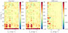 |
Fig. C.1. The average cross-coherence between three different observations covering different local sidereal time (LST) ranges for power spectra obtained from visibilities calibrated with a matched PSO sky model in the left panel, calibrated with a mismatched sky model, that is missing the diffuse Galactic emission component, in the middle panel and the difference between them in the right panel. There is an increase in coherence in (k⊥, k∥)-bins corresponding to short baselines |u|< 100, showing that DI-gain calibration errors due to missing Galactic diffuse emission are partly coherent. |
All Tables
Properties of the simulated dataset based on real LOFAR-HBA observations of the NCP.
All Figures
|
Fig. 1. Sky model of the North Celestial Pole at 141 MHz input to the forward simulations. The flux densities are intrinsic and beam-corrected. It is composed of 684 unpolarized point sources with a flat spectrum. The bright radio source at Dec ∼ 86.3° and RA ∼ 2.5 h is 3C 61.1. |
| In the text | |
|
Fig. 2. Diffuse Galactic emission is modeled as a Gaussian random field with an angular covariance informed by measurements of the NCP at 122 MHz with LOFAR-AARTFAAC data and the Fan Region at 150 MHz with the Westerbork telescope. |
| In the text | |
|
Fig. 3. Normalized histograms of the gain amplitudes at 152 MHz for all stations and time solutions. Solid lines show Rice distribution fits for each calibration scenario. Each panel represents a matrix element of the Jones matrix. The gains are referenced to the core station CS001HBA1 by multiplying them with the inverse gain matrix of CS001HBA1. The blue histogram shows the empirical PDF of gain amplitude solutions for the ground-truth case, obtained by forward-simulating and calibrating with a PSO sky model. The orange histogram shows the empirical PDF for gain solutions from simulations using a PSDE sky model but calibrated with a PSO model, thus omitting diffuse Galactic emission during the DI gain calibration, as described in the text. |
| In the text | |
|
Fig. 4. Top: Baseline lengths for the upper triangle of the visibility matrix. ST denotes Superterp core stations, CS core stations, and RS remote stations; these labels act as proxies for baseline lengths. Baselines < 50 λ and > 5000 λ at an observing frequency of 152 MHz are masked in grey. Middle: Absolute value of the time-averaged gain products for the upper triangle of the visibility matrix in the ground truth scenario. Bottom: Same as the middle panel, but forward-simulating with a PSDE sky model and calibrating with a PSO sky model, thereby neglecting diffuse Galactic emission during DI gain calibration. |
| In the text | |
|
Fig. 5. Left panel: Image of the true sky including point sources and diffuse emission. All images are created at frequency 152 MHz with a minimum and maximum baseline distance of 50λ – 250λ. Middle panel: Diffuse emission with a 4 h track point spread function of LOFAR-HBA applied. Right panel: Residual emission is obtained by subtracting the image created prior to the DI gain calibration from the one created afterward. |
| In the text | |
|
Fig. 6. Fiducial 2D cylindrically averaged power spectra of simulated data from a point source model (left panel), from a diffuse Galactic emission model (middle panel) and from thermal noise (right panel). |
| In the text | |
|
Fig. 7. Systematic bias as a fraction of the thermal noise for a simulation with matched sky model DI gain calibration (forward simulation and calibration with a PSO sky model) in the left panel (setup 1) and with a mismatched sky model DI gain calibration (forward-simulation with a PSDE sky model and calibration with a PSO sky model, which is missing the diffuse Galactic foreground component), in the middle panel and right panel (setups 2 and 3). The systematic bias is estimated from ten power spectra under variation of thermal noise (setup 1), diffuse foregrounds (setup 2), thermal noise and foregrounds (setup 3), respectively, in the visibility simulation. Blue regions indicate that the systematic bias is below the estimated thermal noise and red regions above. |
| In the text | |
|
Fig. 8. Average systematic bias, the expected thermal noise and the error on the thermal noise as a function of observation time for three different regions in the 2D power spectrum space: The foreground dominated region in panel 1 (k∥-bins < 0.2 h Mpc−1), the short baseline region, where diffuse Galactic emission is prominent in panel 2 (k∥-bins > 0.2 h Mpc−1 and k⊥-bins < 0.1 h Mpc−1) and the noise dominated region in panel 3 (k∥-bins > 0.2 h Mpc−1 and k⊥-bins > 0.1 h Mpc−1). In orange we show the expected thermal noise, in dashed black the error on the thermal noise as a function of integration time and in blue and purple the systematic bias for matched PSO and mismatched sky model calibration, respectively. |
| In the text | |
|
Fig. 9. Cross-coherence corner-plot between three different simulated observations covering different local sidereal time (LST) ranges. Top panel: Average cross-coherence when DI gain calibrations are applied to the visibilities with a matched PSO sky model. Bottom panel: Average cross-coherence when DI gain calibrations are applied to the visibilities with an mismatched sky model, which is omitting the diffuse Galactic emission. Three regions of the (k⊥, k∥)-space are analyzed: The foreground region k‖ < 0.2 h Mpc−1 (left panel), and two EoR-windows for k‖ > 0.2 h Mpc−1 and baselines < 100 λ (middle panel), and baselines > 100 λ (right panel). There is on average strong cross-coherence between observations in the foreground region (left panel), whereas weak coherence in the EoR-regions (middle and right panel). There are only minor differences in the average cross-coherence in the EoR-window for baselines < 100 λ, where diffuse Galactic emission is prominent, between calibrating with a matched PSO sky model versus a mismatched one. |
| In the text | |
|
Fig. A.1. The left panel shows the residual emission obtained by differencing the DI-gain calibrated sky from the true sky in our ground truth scenario (i.e., when calibrating with a matched PSO sky model). The right panel shows the residual emission obtained when calibrating with a mismatched sky model. |
| In the text | |
|
Fig. B.1. The systematic bias as a fraction of the thermal noise for matched PSO sky model DI-gain calibration, when the cylindrical Stokes I power spectra are coherently averaged for 1, 2 and 3 observations, respectively. Each observation is 4 hours long and separated by 4 hours in local sidereal time, in order to cover a full day of observation for a symmetric array. |
| In the text | |
|
Fig. B.2. The systematic bias as a fraction of the thermal noise for mismatched sky model DI-gain calibration, when the cylindrical Stokes I power spectra are coherently averaged for 1, 2 and 3 days, respectively. Each observation is 4 hours long and separated by 4 hours in local sidereal time, in order to cover a full day of observation for a symmetric array. |
| In the text | |
|
Fig. C.1. The average cross-coherence between three different observations covering different local sidereal time (LST) ranges for power spectra obtained from visibilities calibrated with a matched PSO sky model in the left panel, calibrated with a mismatched sky model, that is missing the diffuse Galactic emission component, in the middle panel and the difference between them in the right panel. There is an increase in coherence in (k⊥, k∥)-bins corresponding to short baselines |u|< 100, showing that DI-gain calibration errors due to missing Galactic diffuse emission are partly coherent. |
| In the text | |
Current usage metrics show cumulative count of Article Views (full-text article views including HTML views, PDF and ePub downloads, according to the available data) and Abstracts Views on Vision4Press platform.
Data correspond to usage on the plateform after 2015. The current usage metrics is available 48-96 hours after online publication and is updated daily on week days.
Initial download of the metrics may take a while.