| Issue |
A&A
Volume 704, December 2025
|
|
|---|---|---|
| Article Number | A115 | |
| Number of page(s) | 10 | |
| Section | Planets, planetary systems, and small bodies | |
| DOI | https://doi.org/10.1051/0004-6361/202555043 | |
| Published online | 09 December 2025 | |
Langmuir waves observed at comet 67P/Churyumov-Gerasimenko
1
Department of Physics, Umeå University,
901 87
Umeå,
Sweden
2
Swedish Institute of Space Physics,
981 28
Kiruna,
Sweden
3
Department of Mathematics, Physics and Electrical Engineering, Northumbria University,
Newcastle-upon-Tyne,
UK
4
Laboratoire de Physique et Chimie de l’Environnement et de l’Espace (LPC2E), CNRS,
Orléans,
France
5
Laboratoire Lagrange, Observatoire de la Côte d’Azur, Université Côte d’Azur (OCA), CNRS,
Nice,
France
★ Corresponding author: This email address is being protected from spambots. You need JavaScript enabled to view it.
Received:
4
April
2025
Accepted:
4
November
2025
Abstract
In the plasma environment of a comet, waves are generated on vastly different temporal and spatial scales. Wave observations were carried out during the cometary flybys in the 1980s and 1990s as well as by the Rosetta spacecraft which accompanied comet 67P/Churyumov-Gerasimenko between 2014 and 2016. Waves are thought to contribute to the transfer of energy in the ionised coma. One of the fundamental plasma waves observed in space is the Langmuir wave, which appears at or above the electron plasma frequency. The Mutual Impedance Probe of the Rosetta Plasma Consortium (RPC-MIP) recorded frequency spectra of electric field fluctuations in the cometary plasma, and we used these spectra in order to detect and identify Langmuir waves. Langmuir waves were found during the part of the Rosetta mission when the comet was less than 2.65-2.8 AU from the Sun. The Langmuir waves appear near, but always outside, the diamagnetic cavity boundary, in a region where, at much lower frequencies, steepened magnetosonic waves also are present.
Key words: plasmas / waves / methods: observational / comets: general / comets: individual: 67P/Churyumov-Gerasimenko
© The Authors 2025
 Open Access article, published by EDP Sciences, under the terms of the Creative Commons Attribution License (https://creativecommons.org/licenses/by/4.0), which permits unrestricted use, distribution, and reproduction in any medium, provided the original work is properly cited.
This article is published in open access under the Subscribe to Open model. This email address is being protected from spambots. You need JavaScript enabled to view it. to support open access publication.
1 Introduction
Waves are important in plasmas as they transfer energy, and they take on a role in energy dissipation by heating the ionised particle populations (Krall & Trivelpiece 1973; Treumann & Baumjohann 1997). Observations of waves in plasmas can often provide information about the properties of the plasma itself, both at the location of an observation, the source region of the waves, and the space through which the waves have travelled (Tsurutani & Oya 1989). At comets, a number of different waves on vastly different temporal and spatial scales were found during the flybys of 1P/Halley and 21P/Giacobini-Zinner in the 1980s (Scarf 1989), and 26P/Grigg-Skjellerup in the 1990s (Neubauer et al. 1993; Volwerk et al. 2013). The present paper concerns observations of Langmuir waves, which are electrostatic waves in a plasma with a frequency of the order of the electron plasma frequency.
The Rosetta spacecraft (Glassmeier et al. 2007a) spent two years accompanying comet 67P/Churyumov-Gerasimenko (henceforth comet 67P) from August 2014 until the end of September 2016. Rosetta was the first spacecraft orbiting a comet, as all the comet encounters in the 1980s and 1990s were fast flybys. The plasma physical aspects of the Rosetta mission were reviewed by Goetz et al. (2022a). Plasma waves were observed throughout the time Rosetta spent at the comet. To put our new observations in context, we briefly review previous wave observations during the different phases of cometary development in chronological order. Soon after Rosetta’s arrival at comet 67P in August 2014, singing comet waves were detected. The singing comet waves are magnetic field oscillations below 100 mHz that have wavelength between 100 km and 700 km (Richter et al. 2015, 2016). The singing comet waves have been observed as far out as 800 km from the nucleus (Goetz et al. 2020). Still early in the mission, in January 2015, ion acoustic waves were observed at a 28 km cometocentric distance (Gunell et al. 2017b). Ion acoustic waves were also detected during the close flyby of 28 March 2015, when the spacecraft reached down to a 15 km cometocentric distance (Gunell et al. 2021).
Shortly after the close flyby, the comet transitioned into a topologically different regime, where a solar wind ion cavity formed, that is to say, a region around the nucleus into which the solar wind ions cannot reach (Behar et al. 2017; Simon Wedlund et al. 2019). Further inside the solar wind ion cavity, another cavity is situated, namely the diamagnetic cavity, which is a region of space around the nucleus where the magnetic field is close to zero. The diamagnetic cavity at comet 67P, in which the magnetic flux density could be determined to be below 1 nT, was first observed by Goetz et al. (2016b). From April 2015 until February 2016, Rosetta encountered the diamagnetic cavity approximately 700 times. Many of these encounters occurred in the months around the perihelion passage on 13 August 2015 (Goetz et al. 2016a). Most of the time, the diamagnetic cavity was located inside the solar wind ion cavity. In a few events, solar wind ions were seen inside the diamagnetic cavity, which was interpreted as a result of the interplanetary magnetic field (IMF) being parallel to the solar wind velocity (Goetz et al. 2023). This interpretation was supported by simulations that showed that for a parallel IMF, there is neither a solar wind ion cavity nor a bow shock (Gunell et al. 2024).
During a large part of the mission, the Rosetta spacecraft was located at cometocentric distances between 100 km and 400 km, where the diamagnetic cavity boundary moved past the spacecraft position many times. Thus, the vicinity of the diamagnetic cavity boundary was probed extensively, and a number of different waves were found both inside and outside of it. Gunell et al. (2017a) found ion acoustic waves peaking at approximately 200 Hz whenever Rosetta was inside the cavity. Madsen et al. (2018) examined intervals around Rosetta spacecraft crossings of the diamagnetic cavity boundary, and they observed lower hybrid waves at a frequency of a few hertz outside the diamagnetic cavity and ion acoustic waves at the same frequency on the inside of the diamagnetic cavity boundary.
One type of wave that has a significant influence on the plasma density as well as the magnetic field in the inner coma is known as a steepened wave (Stenberg Wieser et al. 2017). These waves appear close to the diamagnetic cavity boundary, but always on the outside. They have periods of a few minutes and are characterised first by a rise in magnetic field and density by a factor of 2–5 for approximately 20 s. This is followed by a decay over 2–3 min (Stenberg Wieser et al. 2017; Engelhardt et al. 2018; Ostaszewski et al. 2021). In a statistical study of Rosetta data from December 2014 to June 2016, Ostaszewski et al. (2021) interpreted the steepened waves as magnetosonic waves propagating in a direction perpendicular to the magnetic field. The large difference between the minima and maxima in the magnetic field and density of the waves creates significant gradients in both of these quantities. A few unusual density enhancements have been reported inside the diamagnetic cavity (Hajra et al. 2018). They were not accompanied by any magnetic field enhancement as the magnetic field in the cavity remained close to zero. The shape of the density enhancements resembles the steepened waves, and the authors speculated that they could have been transmitted through the boundary from the outside. However, what the transmission mechanism might be remains an open question.
Other waves of a shorter and faster length and timescale have been observed when the spacecraft was situated on those gradients. Odelstad et al. (2020) observed waves with periods of the order of 10 s predominantly in the plasma density, but in some cases the waves were also seen as fluctuations of the magnetic field. These waves were classified as ion Bernstein waves. On an even faster timescale, several authors have reported waves in the lower hybrid frequency range (1–10 Hz approximately) (Karlsson et al. 2017; André et al. 2017; Stenberg Wieser et al. 2017).
Myllys et al. (2021) surveyed ‘electric field emissions’ near the plasma frequency, indicative of Langmuir waves, throughout the time that the Rosetta spacecraft spent near comet 67P, using the passive mode of the mutual impedance probe RPC-MIP (Trotignon et al. 2007). Such wave emissions were found in approximately 1% of the recorded spectra. The highest occurrence rates were found on days near perihelion and in connection with the passage of stream interaction regions and coronal mass ejections. In the 1980s, wave activity near the plasma frequency, which is an indication of Langmuir waves, was recorded in flybys of comet 1P/Halley (Grard et al. 1986) and 21P/Giacobini-Zinner (Kennel et al. 1986).
The Langmuir wave (Langmuir 1928) is a longitudinal wave in a plasma, appearing at and above the electron plasma frequency. Langmuir waves may be generated by electron beam– plasma interactions (see for example Briggs 1964) or through current-driven instabilities (e.g. Sauer & Sydora 2015). In collisionless plasma, Langmuir waves constitute one of the ways in which energy can be transferred between particle populations that otherwise would not interact. The occurrence and the role of Langmuir waves in plasmas throughout the solar system was reviewed by Briand (2015).
In this paper, we use the RPC-MIP instrument to observe Langmuir wave spectra in the plasma outside the diamagnetic cavity of comet 67P, and we examine the relationship between these Langmuir waves and the previously reported steepened waves. The instrumentation, data processing and statistical methods are described in Sect. 2; the observations including waves, plasma environment, and statistics are reported in Sect. 3; a possible explanation for the observed waves is discussed in Sect. 4, and the conclusions are summarised in Sect. 5.
2 Instrumentation and data processing
2.1 Instrumentation
In this work, we have used data acquired by instruments belonging to the Rosetta Plasma Consortium (RPC) (Carr et al. 2007). The wave spectra were obtained by the Mutual Impedance Probe (RPC-MIP) (Trotignon et al. 2007) operating in its passive mode. In the passive mode RPC-MIP measures the voltage between two 8 cm long cylindrical electrodes mounted 1 m apart on the boom of Langmuir probe 1, at a distance larger than 12 cm from the boom axis. A Fourier spectrum analysis is performed onboard and the spectrum in the range 7 kHz–3.5 MHz is transmitted to ground. The signal is related to the electric field of waves in the plasma. However, as only one component of the electric field is probed, and since any wave field can be distorted by the presence of the spacecraft and/or the boom itself, this must be seen as a relative measurement. The treatment of interference and noise in the spectrum is described in Sect. 2.2.
In its active mode, RPC-MIP transmits from a set of one or two electric sensors an oscillating pulse through the plasma while simultaneously measuring the electric fluctuation that propagate in the plasma with another set of two electric sensors. This procedure enables to identify the plasma eigenmodes, which enables the determination of the plasma frequency and hence also the plasma density. This density is cross-calibrated (Heritier et al. 2017; Breuillard et al. 2019) with data, ion current and floating potential, from the Langmuir probe instrument (RPC-LAP) (Eriksson et al. 2007). The aim is to optimise both accuracy and temporal resolution, and the resulting product is the MIP-LAP dataset (Johansson et al. 2021), which we have used for the plasma densities reported in this work. The magnetic field was measured by the magnetometer (RPC-MAG) (Glassmeier et al. 2007b) and the ion data were provided by the Ion Composition Analyser (RPC-ICA) (Nilsson et al. 2007).
2.2 Data processing
The RPC-MIP spectrograms contain, apart from a desired Langmuir wave signal, notable levels of noise that appear at higher levels in some of the frequency bands. Fig. 1a shows an original passive spectrum obtained by RPC-MIP. The instrument output is colour-coded and shown in decibels, where 0 dB corresponds to 0.6 µV Hz−1/2. In order to highlight the signal, we employed the noise-removal procedure described in Appendix A. The data points in each frequency band shown in Fig. 1a can be modelled as a superposition of statistical noise and a wave signal. We approximated the noise distribution with a modified Poisson distribution, keeping the high amplitude data points, as detailed in Appendix A. As an example, Fig. 1a shows the original spectrum and Fig. 1b the output of the noise removal procedure. For some frequency bands that are particularly prone to noise, as, for example a known interference band at 266 kHz, it is difficult to separate the signal from the noise, because the scheme relies on the power level of the signal being higher than that of the noise. Therefore part of the noise at 266 kHz remains, although the power of that noise has been significantly reduced. In the following we have removed all data in the 266 kHz channel as well as the ones immediately below (252 kHz) and above (280 kHz) it, and we have not included those channels in the analysis.
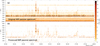 |
Fig. 1 Removal of noise from the RPC-MIP spectrograms. (a) An RPC-MIP spectrum using the original data. (b) A spectrum with the noise removed. The colour scale is normalised so that 0 dB corresponds to 0.6 µV Hz−1/2. |
2.3 Statistical analysis
We used the cleaned data to conduct a statistical analysis. The algorithm described below allowed us to automatically detect the presence of Langmuir waves in the RPC-MIP data set. In a first step, we integrated, for each data point (time instance), the power spectral density (in decibels) over all frequencies considered here, that is, above 300 kHz. Only data points for which that integral had a value above 70 dB kHz after integration were considered for further analysis. The limiting value was chosen to keep most of the observations that may contain Langmuir waves while removing as much noise as possible. Additionally, we removed data points, which meet the limiting criteria only for one single time instance within a 5-point sliding window, unless there were at least three consecutive frequency bins where the power spectral density was larger than the threshold value. The necessary trade-off made in this step is that while it removes noise it can also discard instances of weak or very sporadic wave activity.
In a second step, we used the plasma frequency, calculated from the plasma density obtained from combining data from RPC-MIP and RPC-LAP (Johansson et al. 2021). We only included time periods where high time resolution data were available. The time resolution of the density observations is therefore much higher than the electric field observation, and we decided not to apply any advanced interpolation scheme to associate the plasma density to each electric field observation. Instead, for each RPC-MIP data point identified in the initial filtering, we identified all density observations made during the acquisition of the RPC-MIP electric field spectrum and computed the minimum and maximum plasma frequency (fpe,min, fpe,max) for this time period. To select data points representing Langmuir waves, for each time instance in the RPC-MIP data, we then considered the frequency range between fmin = kmin·fpe,min and fmax = kmax · fpe,max, where kmin = 0.85 and kmax = 1.15. Any signal observed within this frequency band is very likely Lang-muir waves. However, to avoid including noise, we identified as Langmuir waves only those time instances where the power spectral density integrated over this frequency band was at least 50% of the power spectral density integrated over the entire frequency range (above 300 kHz). The results from the statistical analysis are presented in Section 3.3.
3 Results
3.1 Plasma environment
The plasma outside the diamagnetic cavity of comet 67P during the months around perihelion was characterised by a plasma density, 500 cm−3 ≲ ne ≲ 5000 cm−3, i.e. going from a few hundred to a few thousand per cubic centimetre, and a temperature in the approximate range 5 eV ≲ kBTe ≲ 30 eV (Stenberg Wieser et al. 2017; Odelstad et al. 2020). The magnetic field was in the range 10 nT ≲ |B| ≲ 100 nT (Goetz et al. 2017), varying notably within that range as the plasma was subjected to steepened waves. A typical example is shown in Fig. 2.
For the sake of a simple estimate of scales we assume the typical values kBTe = 10 eV, n = 3 × 103 cm−3, and |B| = 40 nT. For such values, we have the electron cyclotron frequency at fce ≈ 1.1 kHz, the plasma frequency fpe ≈ 500 kHz, the thermal speed  , and the electron Larmor radius rLe = vth/(2πfce) ≈ 270 m. Thus, we have fce ≪ fpe, which means that, for the purposes of our wave analysis, we can treat the plasma as unmagnetised. Furthermore, assuming a typical wavelength of λ = 20λDe < 10 m for the Langmuir waves, we obtain λ ≪ rLe, showing that the direct influence of the magnetic field on the Langmuir waves is negligible. However, while there is no direct influence from the magnetic field, an indirect influence is possible, as the processes that set up beams or currents that can generate waves in the plasma are likely to depend on the magnetic field.
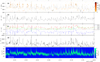 |
Fig. 2 Rosetta data recorded on 31 July 2015 as comet 67P was close to perihelion. (a) Passive spectrum obtained by the RPC-MIP instrument. (b) Magnitude of the magnetic field |B| measured by RPC-MAG. (c) Magnetic field components Bx (blue), By (green), and Bz (red). (d) Plasma density obtained by RPC-MIP and RPC-LAP (see Sect. 2.1) (e) Ion energy spectrogram obtained by RPC-ICA. The colour coded quantity lg (ΓICA) is the logarithm of the differential particle flux in units of cm−2 s−1 sr−1 eV−1 summed over all azimuth angles. |
3.2 Wave observations
Fig. 2 shows Rosetta data recorded during two hours on 31 July 2015. In panel a, the RPC-MIP spectrum, after application of the noise removal technique described in Sect. 2.2, is shown. The grey line shows the plasma frequency calculated from the density (Fig. 2d) data of the cross-calibrated MIP-LAP dataset. Signals around the plasma frequency, indicative of Langmuir waves, can be seen throughout the two-hour period. These signals are more prominent when the density is high, but the signal is not exclusively confined to high density periods, as Fig. 2a shows. Steepened waves are also present during all of the 2 hours shown. These waves are seen in both the magnetic field magnitude (Fig. 2b), in the components of the magnetic field (Fig. 2c), the plasma density (Fig. 2d), and the ion energy spectrum (Fig. 2e). The variations in ion energy indicate that the spacecraft potential is changing as a result of the steepened wave, as previously reported by Stenberg Wieser et al. (2017).
Fig. 3 shows a closeup of a 6-minute interval from 12:07 to 12:13 on 6 September 2015 with the same quantities as in Fig. 2. The electric field RPC-MIP spectrum (Fig. 3a) shows that there is wave activity mostly at and above the local plasma frequency, but at times also below it, for example around 12:08:30. The same tendency as noted in the discussion of Fig. 2 above is seen here: the signal is stronger when the plasma frequency, and therefore also the density, is higher. Steepened waves are seen in both the magnetic field data (Figs. 3b and c), the plasma density (Fig. 3d) and the ion spectrogram (Fig. 3e). However, as the waveform of the steepened waves is somewhat irregular, one cannot find a one to one correspondence between the phase of the steepened waves and the presence of Langmuir waves.
Fig. 4 shows Rosetta data for part of 3 August 2015. Rosetta moved in and out of the diamagnetic cavity many times during that day. The cavity encounters can be recognised as periods of low values of |B| in panel b and low values also of the components of B shown in panel c. The cavity encounters, as identified by Goetz et al. (2016a), have also been marked by grey areas at the top and bottom of each panel, and the diamagnetic cavity boundary was traversed at the times of the vertical grey lines. Panel d shows the plasma density as measured by the Lang-muir probe instrument. The cross-calibrated MIP-LAP dataset was not available for this day. Fig. 4a shows the RPC-MIP passive spectrum, and there are Langmuir wave signals during most of the interval shown. However, all of the wave signals that are at significant levels appear outside of the diamagnetic cavity. During the intervals in Fig. 4 that are inside the cavity only a few low level signals appear, and these do not follow the plasma frequency as the signals outside of the cavity do. The signals in the cavity should therefore rather be regarded as noise that the noise reduction method failed to remove completely. Density enhancements and magnetic field peaks regularly occur as the spacecraft leaves the diamagnetic cavity (Goetz et al. 2016b; Hajra et al. 2018). It is seen in Fig. 4a that also Langmuir waves occur at these times. It is likely that the magnetic field and density peaks appear as a result of the interaction between the steepened waves and the diamagnetic cavity boundary, and that the Langmuir waves follow the steepened waves in the same way as they do at distances further away from the diamagnetic cavity.
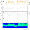 |
Fig. 3 Rosetta data for 6 minutes on 6 September 2015. (a) Passive spectrum obtained by the RPC-MIP instrument. (b) Magnitude of the magnetic field |B| measured by RPC-MAG. (c) Magnetic field components Bx (blue), By (green), and Bz (red). (d) Plasma density obtained by RPC-MIP and RPC-LAP (see Sect. 2.1 (e) Ion energy spectrogram obtained by RPC-ICA. The colour coded quantity lg (ΓICA) is the logarithm of the differential particle flux in units of cm−2s−1sr−1eV−1 summed over all azimuth angles. |
3.3 Statistical study
For the statistical investigation, we consider six hour long time periods. If both RPC-MIP data and high time resolution density from MIP-LAP are simultaneously available during some time intervals during the six hours, we include the six hour block in our analysis. For each included six hour period we compute the occurrence rate τ of Langmuir waves. The occurrence rate is the total time TLangmuir Langmuir waves are observed divided by the total time Tdata when data were available (the time where both density with high time resolution and RPC-MIP data exist). The general definition of τ is thus
 (1)
and the six hour average is denoted τ6h. Typically high time resolution density is not available during all six hours and it should be noted that the occurrence rate is computed from time periods of different lengths.
(1)
and the six hour average is denoted τ6h. Typically high time resolution density is not available during all six hours and it should be noted that the occurrence rate is computed from time periods of different lengths.
In Figure 5 the six hour time periods with data are plotted as a function of heliocentric distance. We used a bin size of 0.005 AU and periods where data are available are shown as blue shaded time intervals. If Langmuir waves are present the computed occurrence rate is shown as black bars. The occurrence rate given is the mean of τ6h in each bin. From Fig. 5 we see that the data covers heliocentric distances from Rosetta’s perihelion at 1.25 AU out to 3.8 AU. Langmuir waves are more often observed for smaller heliocentric distances. To put a quantitative measure to this statement we compare the presence of Langmuir waves for heliocentric distances below and above 2.65 AU. Out of 664 six hour intervals with data observed at heliocentric distances below 2.65 AU (red dashed line in Fig. 5) 459 (corresponding to 69%) contain Langmuir waves. At heliocentric distances above 2.65 AU there are 276 six-hour intervals from which only 26 (9%) have Langmuir waves.
To understand how common Langmuir waves are during the 6 hour intervals when they were detected the occurrence rate τ6h is computed, and it is found to be highly variable. The mean occurrence rate for six-hour blocks containing waves is 1.8%, ranging from 0.02% to 41%. (The occurrence rates seen in Fig. 5 are slightly different due to the re-binning process.) For heliocentric distances below 2.65 AU the mean of τ6h is 1.5% and for the 26 periods at distances above 2.65 AU the mean is 6.3%. This means that while Langmuir waves are more common close to perihelion, they occur for longer time periods on the few occasions when they appear at large heliocentric distances. While the occurrence rate of the Langmuir waves drops sharply at 2.65 AU in our dataset, Fig. 5 shows that there is a gap in the data available for heliocentric distances just above 2.65 AU. Therefore, the transition could in reality be smoother and take place anywhere between 2.65 AU and 2.8 AU.
In Figs. 2 and 3, we see that Langmuir waves are more likely to be observed when the plasma frequency is larger. This also holds statistically for the entire dataset. For 79% of the time where data are available the plasma frequency is below 406 kHz. However, only during 55% of the time when we detect Langmuir waves the plasma frequency falls below 406 kHz. As the plasma frequency increases with increasing density, this means that there is a preference for the Langmuir waves to be observed when the plasma density is high. Additionally, there is a positive correlation between the power in the observed waves and the plasma frequency. This could in part be an instrumental effect: the spectrum is based on a measurement of the voltage between two electrodes separated by a fixed distance (1 m), and for a constant electric field amplitude, shorter wavelengths, and hence higher frequencies, would produce a larger voltage. The observation above that fewer occurrences of Langmuir waves are seen at large heliocentric distances can also be related to this, since farther away from the Sun, the density is lower, which leads to lower frequency waves and lower observed amplitudes. Also, at low plasma density the wave frequency can move below the lower frequency limit for the statistical study of 300 kHz (Sect. 2.3).
4 Discussion
4.1 Wave environment
The environment in which Langmuir waves were detected in this work is characterised by the presence of other waves, most notably steepened waves. These waves have a much lower frequency, and from a Langmuir wave point of view they could be seen as quasi-stationary spatial variations in the plasma density and magnetic field. The foreshock of planets bear some resemblance to this region: there are large amplitude magnetic fluctuations, and Langmuir waves are present (cf. the review by Briand 2015). In the foreshock, the Langmuir waves are generated by interactions between the plasma and electron beams created by acceleration at the bow shock. In our case, the region where we observe the Langmuir waves is not directly connected to a shock, and therefore there must be a different source of free energy to generate the waves. Langmuir waves have also been detected in magnetic holes in the solar wind (Lin et al. 1996; Briand et al. 2010; Briand 2015). The magnetic holes are regions with weaker magnetic fields than the surrounding solar wind plasma. A recent statistical study showed higher occurrence rates of Langmuir waves inside than outside these holes, and that the majority of the Langmuir wave detection are happening at locations with a higher than background plasma density (Boldú et al. 2023). The Strahl electron population of the solar wind could be involved in the generation of the Langmuir waves, but the precise mechanism is not yet determined (Boldú et al. 2023). Thus, the comet case has similarities with but also differences from both the planetary foreshock and the solar wind magnetic hole environments.
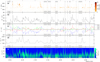 |
Fig. 4 Rosetta data obtained on 3 August 2015, during a period with frequent diamagnetic cavity encounters. The grey boxes and vertical lines on all panels mark these diamagnetic cavity traversals. (a) Passive spectrum obtained by the RPC-MIP instrument. (b) Magnitude of the magnetic field |B| measured by RPC-MAG. (c) Magnetic field components Bx (blue), By (green), and Bz (red). (d) Plasma density obtained by RPC-MIP and RPC-LAP (see Sect. 2.1). (e) Ion energy spectrogram obtained by RPC-ICA. The colour coded quantity lg (ΓICA) is the logarithm of the differential particle flux in units of cm−2 s−1 sr−1 eV−1 summed over all azimuth angles. |
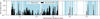 |
Fig. 5 Occurrence rate of Langmuir waves versus heliocentric distance. Six hour long periods are considered and the occurrence rate, τ6h, of Langmuir waves is given as the percent of the time with the required observations during these 6 hours, Langmuir waves are seen. The shaded blue background is the 6 hours long blocks, where both RPC-MIP and MIP-LAP data exist. The vertical red dashed line marks a heliocentric distance of 2.65 AU, discussed further in Sect. 3.3. |
4.2 Possible explanations
Among the waves that can be supported by an electron beam–plasma system we find the Langmuir wave of the background plasma as well as two beam modes, namely the fast space charge wave, travelling faster than the beam and the slow space charge wave, travelling slower than the beam (Briggs 1964). A narrow beam relaxes first into a gentle bump and eventually into a plateau as it is affected by the waves generated by the beam–plasma interaction. When this happens the topology of the dispersion relation changes and beam modes can connect to the Langmuir mode of the background plasma (O’Neil & Malmberg 1968). Another possibility is that of current-driven waves, meaning that the electron distribution itself is stable, but the instability is created by the entire electron distribution moving with respect to the ions. This was seen in simulations by Sauer & Sydora (2015, 2016). Langmuir waves can also be generated by a time-dependent modulation of the distribution function, which changes the electron heating (Briand et al. 2008).
4.3 A beam–plasma example
Given that the timescale of the steepened waves is much longer than that of the electron motion, the density variations of the steepened waves should also be associated with a potential difference. In order to test whether electrons accelerated by this potential difference would be able to generate the observed Langmuir waves calculations using a simple one-dimensional kinetic model are performed in Appendix B. Assuming Boltzmann distributed electrons with a 5 eV temperature, the minimum and maximum densities in Fig. 3, which are used as an example, yields a potential difference of approximately 10 V. This voltage could create an electron beam from the low density, and low potential, side going into the high density, high potential, side. The kinetic calculation in Appendix B shows that this would lead to a distribution that would be unstable, and the slow space charge wave would be growing for a wide range of wave numbers. This beam-type slow space charge wave could then transition into a Langmuir wave as described by O’Neil & Malmberg (1968).
For this scenario to be viable, there must be a component of the steepened wave electric field parallel to the magnetic field, since a perpendicular electric field only would create a slow E × B drift and not an electron beam. The steepened waves are thought to be magnetosonic (Ostaszewski et al. 2021), and such waves could have a parallel electric field component even if that is not necessary. However, as these waves approach the approximately spherical density gradient in the head of the comet, the waves are expected to steepen more near the nucleus, than further out. This would lead to high density peaks near the nucleus, being magnetically connected to lower density regions, and in such a geometry parallel electric fields are likely to form.
A 10 eV electron beam cannot be measured directly, since the spacecraft is negatively charged to a similar potential. However, the conditions for wave generation via this mechanism are there, and this mechanism is consistent with the waves we observe. This would then be a process through which energy is transferred from the large and slow scale of the steepened waves to the small and fast scale of the Langmuir waves and from there into heating of the plasma. We compared the instances of Langmuir waves in this study to list of steepened magnetosonic waves published by Ostaszewski et al. (2021), where the waveforms were identified, using an machine learning technique (Ostaszewski et al. 2020). The Langmuir waves identified in this work coincided with the steepened waveforms identified by Ostaszewski et al. (2021), in 13% of the cases. This number depends not only on the occurrence rates of the two kinds of waves, but also on the definition of when a wave is steep enough to be identified as a steepened wave (Ostaszewski et al. 2020). Also when a magnetosonic wave is not as steep, there can be density variations large enough to enable the proposed mechanism for Langmuir wave generation.
4.4 Verification needs
In this section, we consider what would be needed to verify the beam-plasma interaction mechanism described in Sect. 4.3 or one of the competing explanations discussed in Sect. 4.2 such as current-driven waves or time dependent electron heating. For an observational verification one would need to measure the electron distribution function, resolving both the thermal distribution and any beam or bump on tail. This was not possible on Rosetta due to the negative spacecraft potential.
The Rosetta spacecraft became negatively charged, to a large extent because bus bars on the solar panels were exposed to space. The bus bar cathode was connected to spacecraft ground and the anode was biased at approximately +75 V. At this potential the bus bars pulled in electrons from the plasma, giving the spacecraft a net negative charge. The problem became particularly severe in the dense plasma near the comet nucleus, where the electron population has a cold component (Johansson et al. 2020). This effect can be mitigated when a spacecraft is designed by connecting the anode of the bus bar to spacecraft ground, thereby making the potential of the bus bar negative, which means it will not attract an electron current. This design was used successfully on for example the Atmosphere Explorer and Dynamics Explorer spacecraft (Samir et al. 1979; Zuccaro & Holt 1982).
Any electron scale model for what is causing the Langmuir waves relies on assumptions about the nature of the density gradient associated with the steepened magnetosonic waves. All our knowledge about these waves come from single-spacecraft measurements. In the future, multi-point observations of cometary environments will help to better characterise the environment in which Langmuir waves develop and evolve. An example of a possible multi-spacecraft mission with such capabilities was proposed to ESA’s Voyage 2050 programme by Goetz et al. (2022b). In simulations, to thoroughly determine the cause of the Langmuir wave generation one would have to simulate both the large scale steepened magnetosonic waves and the smaller scale Langmuir waves, including the electrons and resolving plasma period and Debye length scales. That task would be very demanding on the computational resources.
5 Summary and conclusions
We have observed waves in a frequency range of several hundred kilohertz, using the passive mode of the RPC-MIP instrument onboard the Rosetta spacecraft at comet 67P/Churyumov-Gerasimenko. The waves were observed around the local electron plasma frequency, and we interpret them as Langmuir waves. The vast majority of these Langmuir waves were seen when the comet was near its perihelion and out to heliocentric distances of approximately (2.6–2.8) AU. They appear during periods where also the, previously reported, much slower steepened waves (Stenberg Wieser et al. 2017; Engelhardt et al. 2018; Ostaszewski et al. 2021) are seen. The Langmuir waves preferentially occur when the plasma density is in the higher part of the range of density values associated with the steepened waves. This is shown in Sect. 3.3, and preference for higher plasma frequencies, and thus densities, is also visible in Figs. 2 and 3.
We suggest an explanation that is consistent with the available data: that the Langmuir waves are caused by electron beams, moving from the low density, and low potential, region of the steepened waves towards the high density, and high potential, region of these waves. The density variation corresponds to a potential difference of the order of 10 V (Appendix B), and this can generate electron beams capable of causing the observed waves according to estimates made using kinetic theory. For this scenario to play out the electric field associated with the density gradients in the steepened waves must have a significant component parallel to the magnetic field. This can happen in the non-uniform plasma surrounding the comet nucleus, where a highly steepened wave in the density gradient near the nucleus is likely to be magnetically connected to less steepened waves farther away. Experimental verification of this mechanism would require the capability to measure electron beams at energies down to 10 eV or lower, and that was not possible on Rosetta, where the spacecraft potential generally was lower than −10 V.
In the scenario proposed here, Langmuir waves provide a means of transferring energy from the large scale fluctuations of the steepened waves to the smaller Langmuir wave spatial scale and ultimately into heating of the particle populations.
Acknowledgements
The Rosetta data used in this study is available through the ESA Planetary Science Archive (https://www.cosmos.esa.int/web/psa). Computer code used to compute the dispersion relations in the appendix is available at https://cdsarc.cds.unistra.fr/viz-bin/qcat?J/A+A/600/A3. This work was supported by the Swedish National Space Agency contract 2023-00208. This work was supported by CNES APR.
References
- André, M., Odelstad, E., Graham, D. B., et al. 2017, MNRAS, 469, S29 [Google Scholar]
- Behar, E., Nilsson, H., Alho, M., Goetz, C., & Tsurutani, B. 2017, MNRAS, 469, S396 [Google Scholar]
- Boldú, J. J., Graham, D. B., Morooka, M., et al. 2023, A&A, 674, A220 [NASA ADS] [CrossRef] [EDP Sciences] [Google Scholar]
- Breuillard, H., Henri, P., Bucciantini, L., et al. 2019, A&A, 630, A39 [NASA ADS] [CrossRef] [EDP Sciences] [Google Scholar]
- Briand, C. 2015, J. Plasma Phys., 81, 325810204 [CrossRef] [Google Scholar]
- Briand, C., Mangeney, A., & Califano, F. 2008, J. Geophys. Res. (Space Phys.), 113, A07219 [Google Scholar]
- Briand, C., Soucek, J., Henri, P., & Mangeney, A. 2010, J. Geophys. Res. (Space Phys.), 115, A12113 [Google Scholar]
- Briggs, R. J. 1964, Electron-Stream Interaction with Plasmas, Research Monograph, 29 (Cambridge, Massachusetts, USA: MIT Press) [Google Scholar]
- Broiles, T. W., Livadiotis, G., Burch, J. L., et al. 2016, J. Geophys. Res. (Space Phys.), 121, 7407 [Google Scholar]
- Carr, C., Cupido, E., Lee, C. G. Y., et al. 2007, Space Sci. Rev., 128, 629 [Google Scholar]
- Engelhardt, I. A. D., Eriksson, A. I., Stenberg Wieser, G., et al. 2018, MNRAS, 477, 1296 [Google Scholar]
- Eriksson, A. I., Boström, R., Gill, R., et al. 2007, Space Sci. Rev., 128, 729 [Google Scholar]
- Eriksson, A. I., Engelhardt, I. A. D., André, M., et al. 2017, A&A, 605, A15 [NASA ADS] [CrossRef] [EDP Sciences] [Google Scholar]
- Gilet, N., Henri, P., Wattieaux, G., Cilibrasi, M., & Béghin, C. 2017, Radio Sci., 52, 1432 [Google Scholar]
- Glassmeier, K.-H., Boehnhardt, H., Koschny, D., Kührt, E., & Richter, I. 2007a, Space Sci. Rev., 128, 1 [Google Scholar]
- Glassmeier, K.-H., Richter, I., Diedrich, A., et al. 2007b, Space Sci. Rev., 128, 649 [NASA ADS] [CrossRef] [Google Scholar]
- Goetz, C., Koenders, C., Hansen, K. C., et al. 2016a, MNRAS, 462, S459 [NASA ADS] [CrossRef] [Google Scholar]
- Goetz, C., Koenders, C., Richter, I., et al. 2016b, A&A, 588, A24 [NASA ADS] [CrossRef] [EDP Sciences] [Google Scholar]
- Goetz, C., Volwerk, M., Richter, I., & Glassmeier, K.-H. 2017, MNRAS, 469, S268 [NASA ADS] [CrossRef] [Google Scholar]
- Goetz, C., Plaschke, F., & Taylor, M. G. G. T. 2020, Geophys. Res. Lett., 47, e2020GL087418 [Google Scholar]
- Goetz, C., Behar, E., Beth, A., et al. 2022a, Space Sci. Rev., 218, 65 [NASA ADS] [CrossRef] [Google Scholar]
- Goetz, C., Gunell, H., Volwerk, M., et al. 2022b, Exp. Astron., 54, 1129 [NASA ADS] [CrossRef] [Google Scholar]
- Goetz, C., Scharré, L., Simon Wedlund, C., et al. 2023, J. Geophys. Res. (Space Phys.), 128, e2022JA031249 [Google Scholar]
- Grard, R., Pedersen, A., Trotignon, J. G., et al. 1986, Nature, 321, 290 [Google Scholar]
- Gunell, H., Goetz, C., Eriksson, A., et al. 2017a, MNRAS, 469, S84 [NASA ADS] [CrossRef] [Google Scholar]
- Gunell, H., Nilsson, H., Hamrin, M., et al. 2017b, A&A, 600, A3 [NASA ADS] [CrossRef] [EDP Sciences] [Google Scholar]
- Gunell, H., Goetz, C., Odelstad, E., et al. 2021, Ann. Geophys., 39, 53 [CrossRef] [Google Scholar]
- Gunell, H., Goetz, C., & Fatemi, S. 2024, A&A, 682, A62 [NASA ADS] [CrossRef] [EDP Sciences] [Google Scholar]
- Hajra, R., Henri, P., Vallières, X., et al. 2018, MNRAS, 475, 4140 [NASA ADS] [CrossRef] [Google Scholar]
- Heritier, K. L., Henri, P., X. Vallières, X., et al. 2017, MNRAS, 469, S118 [NASA ADS] [CrossRef] [Google Scholar]
- Johansson, F. L., Eriksson, A. I., Gilet, N., et al. 2020, A&A, 642, A43 [NASA ADS] [CrossRef] [EDP Sciences] [Google Scholar]
- Johansson, F. L., Eriksson, A. I., Vigren, E., et al. 2021, A&A, 653, A128 [NASA ADS] [CrossRef] [EDP Sciences] [Google Scholar]
- Karlsson, T., Eriksson, A. I., Odelstad, E., et al. 2017, Geophys. Res. Lett., 44, 1641 [NASA ADS] [Google Scholar]
- Kennel, C. F., Coroniti, F. V., Scarf, F. L., et al. 1986, Geophys. Res. Lett., 13, 921 [Google Scholar]
- Krall, N. A., & Trivelpiece, A. W. 1973, Principles of Plasma Physics (New York: McGraw-Hill) [Google Scholar]
- Langmuir, I. 1928, Proc. Natl. Acad. Sci., 14, 627 [Google Scholar]
- Lin, N., Kellogg, P. J., MacDowall, R. J., Tsurutani, B. T., & Ho, C. M. 1996, A&A, 316, 425 [Google Scholar]
- Löfgren, T., & Gunell, H. 1997, Phys. Plasmas, 4, 3469 [Google Scholar]
- Madsen, B., Simon Wedlund, C., Eriksson, A., et al. 2018, Geophys. Res. Lett., 45, 3854 [NASA ADS] [CrossRef] [Google Scholar]
- Myllys, M., Henri, P., Vallières, X., et al. 2021, A&A, 652, A73 [NASA ADS] [CrossRef] [EDP Sciences] [Google Scholar]
- Neubauer, F. M., Glassmeier, K.-H., Coates, A. J., & Johnstone, A. D. 1993, J. Geophys. Res., 98, 20937 [Google Scholar]
- Nilsson, H., Lundin, R., Lundin, K., et al. 2007, Space Sci. Rev., 128, 671 [NASA ADS] [CrossRef] [Google Scholar]
- Odelstad, E., Eriksson, A. I., André, M., et al. 2020, J. Geophys. Res. (Space Phys.), e2020JA028592 [Google Scholar]
- O’Neil, T. M., & Malmberg, J. H. 1968, Phys. Fluids, 11, 1754 [Google Scholar]
- Ostaszewski, K., Heinisch, P., Richter, I., et al. 2020, Acta Astron., 168, 123 [Google Scholar]
- Ostaszewski, K., Glassmeier, K.-H., Goetz, C., et al. 2021, Ann. Geophys., 39, 721 [Google Scholar]
- Richter, I., Koenders, C., Auster, H.-U., et al. 2015, Ann. Geophys., 1031 [Google Scholar]
- Richter, I., Auster, H.-U., Berghofer, G., et al. 2016, Ann. Geophys., 34, 609 [CrossRef] [Google Scholar]
- Samir, U., Gordon, R., Brace, L., & Theis, R. 1979, J. Geophys. Res., 84, 513 [NASA ADS] [CrossRef] [Google Scholar]
- Sauer, K., & Sydora, R. D. 2015, J. Geophys. Res. (Space Phys.), 120, 235 [Google Scholar]
- Sauer, K., & Sydora, R. D. 2016, Geophys. Res. Lett., 43, 7348 [NASA ADS] [CrossRef] [Google Scholar]
- Scarf, F. 1989, Plasma Waves and Instabilities at Comets and in Magnetospheres (Washington, DC: American Geophysical Union Geophysical Monograph Series), 53, 31 [Google Scholar]
- Simon Wedlund, C., Behar, E., Kallio, E., et al. 2019, A&A, 630, A36 [NASA ADS] [CrossRef] [EDP Sciences] [Google Scholar]
- Stenberg Wieser, G., Odelstad, E., Nilsson, H., et al. 2017, MNRAS, 469, S522 [NASA ADS] [CrossRef] [Google Scholar]
- Treumann, R. A., & Baumjohann, W. 1997, Advanced Space Plasma Physics (Imperial College Press) [Google Scholar]
- Trotignon, J. G., Michau, J. L., Lagoutte, D., et al. 2007, Space Sci. Rev., 128, 713 [NASA ADS] [CrossRef] [Google Scholar]
- Tsurutani, B. T., & Oya, H., eds. 1989, Plasma Waves and Instabilities at Comets and in Magnetospheres, 53 (Washington, DC: American Geophysical Union Geophysical Monograph Series) [Google Scholar]
- Volwerk, M., Koenders, C., Delva, M., et al. 2013, Ann. Geophys., 31, 2201 [Google Scholar]
- Wattieaux, G., Henri, P., Gilet, N., Vallières, X., & Deca, J. 2020, A&A, 638, A124 [NASA ADS] [CrossRef] [EDP Sciences] [Google Scholar]
- Zuccaro, D. R., & Holt, B. J. 1982, J. Geophys. Res., 87, 8327 [NASA ADS] [CrossRef] [Google Scholar]
Appendix A Noise reduction scheme
The dataset from RPC-MIP is a 2-dimensional matrix of even integer numbers, noted as  with
with  , and f and t indicating the time and frequency bin numbers, respectively. We define the Poisson distribution modified to account only for even integers as
 (A.1)
with
(A.1)
with  the digitised signal strength. The signal strength reported by the instrument is assumed to follow the aforementioned distribution, cf,t~PoisMod(λf,t), with λf,t the measured signal in the frequency band f and time t. The wave signal
  and background noise
  both contribute to the observed signal strength, such that
  . At every frequency band, the measured signal is calculated using a maximum likelihood estimation from the observation of data within a time window about 20 min long and sliding over time, with a time stepping of about 2 min. The sliding window allows to gather enough statistics for the estimation of λf,t while scanning in fine steps the observation period. The duration and stepping of the sliding window were derived heuristically.
It is now assumed that the signal strength is greater than zero rarely enough to write  , with med the median of all observations within a time window. The frequency band at 1064 kHz, henceforth labelled the reference band, is assumed to consist only of a background signal with strength λref,t. Another fundamental assumption is that there is a linear relationship between λref,t and
  , unique for all frequency bands. The matrix
  ,
,
 (A.2)
contains the intensity of the noise level with respect to the reference band. The noise for any frequency band can therefore be derived as
(A.2)
contains the intensity of the noise level with respect to the reference band. The noise for any frequency band can therefore be derived as  .
.
The data are finally filtered by a likelihood rejection scheme, defined by
 (A.3)
with α = 0.05 the significance level of the rejection. The noise-reduced dataset is showcased in Fig. 1, along with the original. The rejection scheme, however, degrades the foreground signal and can even completely remove it when λs = λbg.
(A.3)
with α = 0.05 the significance level of the rejection. The noise-reduced dataset is showcased in Fig. 1, along with the original. The rejection scheme, however, degrades the foreground signal and can even completely remove it when λs = λbg.
Appendix B Sample dispersion relation
In this appendix, we first determine the potential difference between the high and low density points of a steepened wave, assuming a Boltzmann distribution. Then, we use a one-dimensional kinetic model to see whether electrons accelerated by that potential drop could cause a beam–plasma instability that, in turn, could cause the generation of the observed Langmuir waves.
We assume the density fluctuations of the steepened waves are also associated with potential fluctuations and that the electrons follow a Boltzmann distribution. As an example of a typical
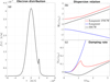 |
Fig. B.1 Dispersion relation calculation illustration, showing (a) distribution function of an electron beam–plasma system, (b) dispersion relation, and (c) damping rate. The black curves show the slow space charge wave (SSCW), the red curves show the fast space charge wave (FSCW) for large values of k and that connects to the forward travelling Langmuir wave for small k. The blue curves show the backward travelling Langmuir wave. |
steepened wave we use interval shown in Fig. 3. For the low density – and hence low potential – side, we pick the density from 2015-09-06 at 12:10:17, which is nl = 7.28 × 10⁸ m−3. The density on the high potential side nh = 5.76 × 10⁹ m−3 is taken at 12:10:35. The energy equivalent of the electron temperature is assumed to be kBTe = 5 eV, where Te is the temperature and kB is Boltzmann’s constant. This is in the range of commonly observed temperatures when the comet was near perihelion (Broiles et al. 2016; Eriksson et al. 2017; Gilet et al. 2017; Wattieaux et al. 2020). The Boltzmann distribution is
 (B.1)
where e is the elementary charge and after rearranging the potential difference ∆V becomes
(B.1)
where e is the elementary charge and after rearranging the potential difference ∆V becomes
 (B.2)
(B.2)
With the above-mentioned densities of our example we obtain ∆V ≈ 10.3 V.
The part of the electron distribution on the low potential side which is moving towards the high potential side will be accelerated by the approximately 10 V potential drop. Liouville mapping of this distribution enables us to estimate its density and temperature after it has been accelerated and superimposed on the denser plasma on the high potential side. An approximation of the resulting beam–plasma or bump-on-tail distribution is shown in Fig. B.1a.
The distribution used here is a superposition of two population, representing the kBTe = 5 eV background plasma and a kBTe = 0.05 eV beam, which is moving at v0 = 2 × 10⁶ m s−1 relative the background. The beam density is 1.5% ×of the total (background + beam) density. The two components are modelled using simple pole expansions (Löfgren & Gunell 1997). Each population is represented by 1 divided by a truncated Taylor expansion to obtain an approximate Maxwellian:
 (B.3)
where vt is the thermal speed. The distribution in (B.3) approaches a Maxwellian as m tends to infinity. For finite values of m, f(v) has thicker tails than the Maxwellian distribution. In our example we have used m = 3 for the beam and m = 5 for the background population. The dispersion relation is computed using the method described by Löfgren & Gunell (1997), and a computer code that can perform the computations is available at <https://cdsarc.cds.unistra.fr/viz-bin/qcat?J/A+A/600/A3>.
(B.3)
where vt is the thermal speed. The distribution in (B.3) approaches a Maxwellian as m tends to infinity. For finite values of m, f(v) has thicker tails than the Maxwellian distribution. In our example we have used m = 3 for the beam and m = 5 for the background population. The dispersion relation is computed using the method described by Löfgren & Gunell (1997), and a computer code that can perform the computations is available at <https://cdsarc.cds.unistra.fr/viz-bin/qcat?J/A+A/600/A3>.
The plasma population is associated with two Langmuir waves, travelling in opposite directions. The beam is associated with the fast and slow space charge waves (Briggs 1964). We solve the dispersion equation for real k and complex ω, and we apply the convention where a positive imaginary part of ω corresponds to damped waves and a negative imaginary part to growing waves. The real part of ω as a function of k represents the dispersion relation, and it is shown in Fig. B.1b. The black curve represents the slow space charge wave, travelling slower than the beam. The fast space charge wave, represented by the red curve for kλDe ≳ 1.2 connects to the forward, in the direction of the beam, travelling Langmuir wave for kλDe ≲ 1.2. The blue curve shows the backward travelling Langmuir wave.
Fig. B.1c shows the imaginary part of ω, which represents the damping rate. The two Langmuir waves are weakly damped in the long wavelength limit, i.e. small values of k, and the fast space charge wave, red curve for kλDe ≳ 1.2, is heavily damped. The slow space charge wave, shown by the black curve, is unstable over a wide range of k values, and this would lead to growing waves in the plasma. As seen in Fig B.1 the fastest growing mode occurs for kλDe ≈ 1, meaning that the wavelength would be λ ≈ 2πλDe. If the beam density is lowered from the value in the example, an unstable mode remains present as long as the beam density is above 0.5%.
The density ratio, nh/nl ≈ 8, used in the numerical example presented here, is in the higher range of what is shown in Figs. 2 and 3. For lower density ratios the acceleration voltage is lower than in our example, but on the other hand, the relative beam density is higher due to both the lower acceleration and that the density ratio was lower from the start. We repeated the calculation for a density ratio of 3, and found that the resulting distribution also was unstable.
All Figures
|
Fig. 1 Removal of noise from the RPC-MIP spectrograms. (a) An RPC-MIP spectrum using the original data. (b) A spectrum with the noise removed. The colour scale is normalised so that 0 dB corresponds to 0.6 µV Hz−1/2. |
| In the text | |
|
Fig. 2 Rosetta data recorded on 31 July 2015 as comet 67P was close to perihelion. (a) Passive spectrum obtained by the RPC-MIP instrument. (b) Magnitude of the magnetic field |B| measured by RPC-MAG. (c) Magnetic field components Bx (blue), By (green), and Bz (red). (d) Plasma density obtained by RPC-MIP and RPC-LAP (see Sect. 2.1) (e) Ion energy spectrogram obtained by RPC-ICA. The colour coded quantity lg (ΓICA) is the logarithm of the differential particle flux in units of cm−2 s−1 sr−1 eV−1 summed over all azimuth angles. |
| In the text | |
|
Fig. 3 Rosetta data for 6 minutes on 6 September 2015. (a) Passive spectrum obtained by the RPC-MIP instrument. (b) Magnitude of the magnetic field |B| measured by RPC-MAG. (c) Magnetic field components Bx (blue), By (green), and Bz (red). (d) Plasma density obtained by RPC-MIP and RPC-LAP (see Sect. 2.1 (e) Ion energy spectrogram obtained by RPC-ICA. The colour coded quantity lg (ΓICA) is the logarithm of the differential particle flux in units of cm−2s−1sr−1eV−1 summed over all azimuth angles. |
| In the text | |
|
Fig. 4 Rosetta data obtained on 3 August 2015, during a period with frequent diamagnetic cavity encounters. The grey boxes and vertical lines on all panels mark these diamagnetic cavity traversals. (a) Passive spectrum obtained by the RPC-MIP instrument. (b) Magnitude of the magnetic field |B| measured by RPC-MAG. (c) Magnetic field components Bx (blue), By (green), and Bz (red). (d) Plasma density obtained by RPC-MIP and RPC-LAP (see Sect. 2.1). (e) Ion energy spectrogram obtained by RPC-ICA. The colour coded quantity lg (ΓICA) is the logarithm of the differential particle flux in units of cm−2 s−1 sr−1 eV−1 summed over all azimuth angles. |
| In the text | |
|
Fig. 5 Occurrence rate of Langmuir waves versus heliocentric distance. Six hour long periods are considered and the occurrence rate, τ6h, of Langmuir waves is given as the percent of the time with the required observations during these 6 hours, Langmuir waves are seen. The shaded blue background is the 6 hours long blocks, where both RPC-MIP and MIP-LAP data exist. The vertical red dashed line marks a heliocentric distance of 2.65 AU, discussed further in Sect. 3.3. |
| In the text | |
|
Fig. B.1 Dispersion relation calculation illustration, showing (a) distribution function of an electron beam–plasma system, (b) dispersion relation, and (c) damping rate. The black curves show the slow space charge wave (SSCW), the red curves show the fast space charge wave (FSCW) for large values of k and that connects to the forward travelling Langmuir wave for small k. The blue curves show the backward travelling Langmuir wave. |
| In the text | |
Current usage metrics show cumulative count of Article Views (full-text article views including HTML views, PDF and ePub downloads, according to the available data) and Abstracts Views on Vision4Press platform.
Data correspond to usage on the plateform after 2015. The current usage metrics is available 48-96 hours after online publication and is updated daily on week days.
Initial download of the metrics may take a while.