| Issue |
A&A
Volume 704, December 2025
|
|
|---|---|---|
| Article Number | A225 | |
| Number of page(s) | 12 | |
| Section | Extragalactic astronomy | |
| DOI | https://doi.org/10.1051/0004-6361/202555188 | |
| Published online | 12 December 2025 | |
Revisiting 3C 279 jet morphology with space VLBI at 26 microarcsecond resolution
1
Instituto de Astrofísica de Andalucía-CSIC, Glorieta de la Astronomía s/n, E-18008 Granada, Spain
2
Max-Planck-Institut für RadioAstronomie, Auf dem Hügel 69, D-53121 Bonn, Germany
3
INAF Istituto di RadioAstronomia, Via Gobetti 101, 40129 Bologna, Italy
4
Aalto University Department of Electronics and Nanoengineering, PL 15500 00076 Aalto, Germany
5
Aalto University Metsähovi Radio Observatory, Metsähovintie 114, 02540 Kylmälä, Finland
6
Crimean Astrophysical Observatory, 298409 Nauchny, Crimea
7
Astro Space Centre of Lebedev Physical Institute, Profsoyuznaya 84/32, Moscow, 117997, Russia
8
Interdisziplinäres Zentrum für Wissenschaftliches Rechnen (IWR), Universität Heidelberg, Im Neuenheimer Feld 205, 69120 Heidelberg, Germany
9
Joint Institute for VLBI ERIC (JIVE), Oude Hoogeveensedijk 4, 7991 PD Dwingeloo, The Netherlands
10
Faculty of Aerospace Engineering, Delft University of Technology, Kluyverweg 1, 2629 HS Delft, The Netherlands
11
Shanghai Astronomical Observatory, Chinese Academy of Sciences, 80 Nandan Rd., Shanghai 200030, China
12
Institute of Astrophysics, Foundation for Research and Technology – Hellas, N. Plastira 100, Voutes, GR-70013 Heraklion, Greece
13
University of Crete, Department of Physics & Institute of Theoretical & Computational Physics, 70013 Heraklion, Greece
14
Instituto de Física, Pontificia Universidad Católica de Valparaíso, Casilla, 4059 Valparaíso, Chile
★ Corresponding author: This email address is being protected from spambots. You need JavaScript enabled to view it.
Received:
17
April
2025
Accepted:
3
October
2025
Abstract
We present observations of the blazar 3C 279 at 22 GHz by the space-based very long baseline interferometry mission RadioAstron from January 15, 2018. We reconstructed images in both total intensity and fractional polarization using the regularized maximum likelihood method implemented in the eht-imaging library. The electric vector position angles are found to be mostly aligned with the general jet direction, suggesting a predominantly toroidal magnetic field and in agreement with the presence of a helical magnetic field. Ground-space fringes were detected up to a projected baseline length of ∼8 Gλ, achieving an angular resolution of around 26 μas. The fine-scale structure of the relativistic jet is found in our study to extend to a projected distance of ∼180 parsec from the radio core. However, the filamentary structure reported by previous RadioAstron observations from 2014 is not detected in our current study. We discuss potential causes for this phenomenon and present a comparison using public 43 GHz data from the BEAM-ME program showing a significant drop in the jet’s total intensity. We observe that the optically thick core has a brightness temperature of 1.6 × 10¹² K, consistent with equipartition between the energy densities of the relativistic particles and the magnetic field. This yields an estimated magnetic field strength of 0.2 G.
Key words: polarization / techniques: high angular resolution / techniques: image processing / techniques: interferometric / galaxies: active / galaxies: jets
© The Authors 2025
 Open Access article, published by EDP Sciences, under the terms of the Creative Commons Attribution License (https://creativecommons.org/licenses/by/4.0), which permits unrestricted use, distribution, and reproduction in any medium, provided the original work is properly cited.
This article is published in open access under the Subscribe to Open model. This email address is being protected from spambots. You need JavaScript enabled to view it. to support open access publication.
1. Introduction
The blazar 3C 279 (1253−055) at redshift z = 0.536 (Marziani et al. 1996) is a bright, highly polarized, and well-monitored source. It is one of the first objects to provide evidence of rapid structure variability (Knight et al. 1971) and apparent superluminal motions in compact active galactic nucleus (AGN) jets (Whitney et al. 1971; Cohen et al. 1971). Since the discovery of the blazar, the structure of the jet in 3C 279, composed of a compact core and a jet extended from sub-parsec to kiloparsec scales, has been thoroughly studied across the whole accessible electromagnetic spectrum, showing high variability and frequent flares. The core of 3C 279 has a high brightness temperature at centimeter wavelengths (e.g., ≳1012 K in Kovalev et al. 2005) as well as a high fractional linear polarization in the jet (≳10%, Pushkarev et al. 2023). In the extended jet, different components show a wide range of apparent speeds (from a few to ∼20c) and a bulk Lorentz factor in the range of Γ ∼ 10–40 (Bloom et al. 2013; Jorstad et al. 2017; Weaver et al. 2022), suggesting the presence of features associated with propagating shocks or instabilities.
Studying the formation, acceleration, or collimation of relativistic jets together with their connection with supermassive black holes (SMBHs) continues to be one of the most extensive pursuits in modern astrophysics (see, e.g., Boccardi et al. 2017; Blandford et al. 2019, and references therein for recent reviews). Different theoretical models have been proposed to interpret this connection, mainly represented by two scenarios (not mutually exclusive) that suggest that either relativistic AGN jets are driven by the conversion of the rotational energy of the black hole to Poynting flux via magnetic field lines, which are attached to the black hole ergosphere (Blandford & Znajek 1977), or that these jets are instead driven by strong magnetic fields anchored onto the black hole accretion disk (Blandford & Payne 1982).
Very long baseline interferometry (VLBI) is a powerful technique that provides great angular resolution, enabling us to resolve and analyze the fine structure of extragalactic jets on (sub-)parsec scales. By observing at higher frequencies or extending the baseline length of the array elements, VLBI enables the study of jet features located at ∼103 Schwarzschild radii from the central engine for a number of AGN sources. In particular, polarimetric VLBI observations play a crucial role in studying extragalactic jets, providing essential insights into jet physics and the configuration of magnetic fields (e.g., Gómez et al. 2001, 2016; Gabuzda 2021; Gómez et al. 2022).
Different monitoring campaigns, such as BEAM-ME (Jorstad et al. 2017) and MOJAVE (Homan et al. 2021; Lister et al. 2021) have successfully and extensively observed these jets at millimeter and centimeter wavelengths, respectively. Particularly for 3C 279, the MOJAVE program, monitoring at 15 GHz, has reported in this source maximum apparent speeds of up to ∼20c, which is consistent with a jet oriented at a small angle to the line of sight and moving with a Lorentz factor of around Γ ∼ 13 (Lister et al. 2019). Similarly, BEAM-ME at 43 GHz has observed component speeds ranging from ∼4c to ∼21c (Jorstad et al. 2017). Other findings using the Very Long Baseline Array (VLBA) have reported a dramatic change in the trajectory of a superluminal component (C4) as well as an apparent projected speed and direction moving with a Lorentz factor of ∼15, suggesting that the trajectory change is a collimation event occurring at around 1 kpc (deprojected) from the core (Homan et al. 2003).
The Event Horizon Telescope (EHT), composed of millimeter wavelength radio telescopes distributed over the globe, provided the first images of black hole shadows with the sharp resolution of ∼20 μas (EHTC 2019a, 2022a). EHT also imaged 3C 279, presenting the first 1.3 mm VLBI images at the extreme angular resolution of 20 μas (Kim et al. 2020), whose results reveal a multicomponent inner jet morphology; the northernmost component elongated nearly perpendicularly to the direction of the jet and separated from the other component by ∼100 μas. This is interpreted as either a broad resolved jet base or a spatially bent jet with low apparent (Tb, obs ≲ 1011 K) and intrinsic brightness temperatures (Tb, int ≤ 1010 K).
The RadioAstron space VLBI mission (Kardashev et al. 2013), which was specifically designed to study ultra compact regions in space objects (Kovalev et al. 2020), operated between 2011 and 2019. Led by the Astro Space Center of Lebedev Physical Institute and the Lavochkin Association, this mission featured a 10 m radio telescope on board the Spektr-R satellite equipped with dual polarization receivers operating at 0.32 GHz (P band), 1.6 GHz (L-band), 4.8 GHz (C-band), and 22 GHz (K-band). With an apogee close to 350 000 km, the observations with RadioAstron enabled the imaging of blazar jets in both total and linearly polarized intensity with unprecedented resolution, that is, of the order of a few tens of microarcseconds (e.g., Lobanov et al. 2015; Gómez et al. 2016; Giovannini et al. 2018; Vega-García et al. 2020; Bruni et al. 2021; Gómez et al. 2022; Savolainen et al. 2023).
The launching, collimation, and magnetic field properties of AGN jets have been studied as part of AGN Imaging Key Science Programmes (KSP) and complemented by the AGN survey on the brightness temperature of their cores (Lobanov 2015; Kovalev et al. 2016). The RadioAstron Polarization KSP constantly collected data throughout the whole duration of the space VLBI mission, successfully probing the regions of the jet closest to the core as well as their magnetic field for a sample of the most energetic blazars. Results of the RadioAstron mission can be found for several sources such as BL Lac (Gómez et al. 2016), 3C 84 (Savolainen et al. 2023), and OJ 287 (Gómez et al. 2022; Cho et al. 2024; Traianou et al. 2025), among others. The blazar 3C 279 was among the sources included in the RadioAstron Polarization KSP, yielding the first robust detection and imaging of a filamentary structure of the jet (Fuentes et al. 2023).
Results from Fuentes et al. (2023) showed for the first time the presence of filaments in the 3C 279 radio jet. These bright filaments are suggested to be compressed regions with enhanced gas and magnetic pressure, likely as a result of Kelvin-Helmholtz (KH) instabilities. Moreover, these filaments exhibit periodic structures and brightness variations attributed to Doppler boosting. This periodicity also matches features observed at 7 mm (Jorstad et al. 2017; Weaver et al. 2022) and likely originates from an elliptical surface mode in a kinetically dominated cold jet. In addition, the source polarization signature discussed in their work indicates the presence of a toroidal magnetic field rotating clockwise along the flow with a pitch angle of −45° and an estimated bulk Lorentz factor of ∼13 (Jorstad et al. 2005; Fuentes et al. 2023).
In this work, we present an investigation of 3C 279 at 22 GHz using RadioAstron observations of this source performed on January 15, 2018, to explore the jet structure, polarization, and time evolution of the filamentary structure previously detected in the 2014 observations (Fuentes et al. 2023). In the following sections, we present the total intensity and polarization images of 3C 279 at 22 GHz obtained with the space-VLBI mission RadioAstron, obtained with the data described in Sect. 2. Moreover, a supplementary study is introduced in different subsections showing the relation with gamma-rays (Sect. 3.2), tests on synthetic data (Sect. 3.3), brightness evolution from the public BEAM-ME 43 GHz VLBA data (Sect. 3.4), a comparison with the previous RadioAstron data from 2014 (Sect. 3.1), and a brightness temperature analysis (Sect. 3.5).
2. Observations and data analysis
The observations (project code: GG083B) were carried out on January 15, 2018, using 14 ground-based radio telescopes and the RadioAstron space radio telescope (see Table 1) at a frequency of 22.22 GHz (1.3 cm, K-band). The polarization calibration was carried out with the source 3C 279 (see Sect. 2.2). The observations were carried out in two sessions with two distinct antenna arrays spanning from 00:49:50 UTC on January 15 to 00:30:45 UTC on January 16, 2018, with a four-hour gap (from 10:00 to 14:00 UTC) during which no observations were made. The data were recorded in both left (LCP) and right (RCP) circular polarization using four intermediate frequencies (IFs) with a recorded bandwidth of 16 MHz each (i.e., a total bandwidth of 64 MHz)
List of observing radio telescopes.
2.1. Data reduction
The raw data were correlated at the Max-Planck-Institute for Radio Astronomy using the RadioAstron dedicated version of the DiFX software correlator (Bruni et al. 2016). Initial data calibration and processing were performed using the NRAO Astronomical Image Processing System (AIPS; Greisen 2003), employing the ParselTongue interface (Kettenis et al. 2006), calibrating first the ground array, and then adding the space antenna.
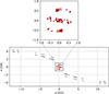 |
Fig. 1. Coverage in the (u,v) plane of the fringe-fitted interferometric visibilities of 3C 279 observed by RadioAstron at 22 GHz on January 15, 2018. The top panel shows only the ground baselines, while the bottom panel shows all baselines, with those of RadioAstron in gray. |
The gap during the observation naturally led to splitting the data into two subsets for separate calibration. For each subset, the same calibration process was applied, i.e., correcting for the parallactic angle and opacity for the ground stations.
An a priori calibration of the correlated visibility amplitudes was performed based on the system temperatures and gain curves recorded at each station. Since six ground antennas (AT, BD, CD, SV, T6, and ZC) did not provide system temperature information, we used the default (average) nominal values provided by each station and modulated them by the antenna’s elevation at each scan. We then solved for residual single- and multi-band delays, phase offsets, and phase rates by fringe-fitting the data using AIPS task FRING.
In the initial stage, we calibrated first only the ground array, and a global fringe fit with an exhaustive baseline search was performed on the ground array with a solution interval of 60 seconds. EF and T6 served as the reference antennas for the first and second data subsets, respectively.
Once the ground array was calibrated, we accounted for the lower sensitivity of the longest projected baselines by adopting different solution intervals (60s and 120s) and combining IFs and polarizations. Afterward, to enhance fringe detection sensitivity on the longer RadioAstron space-ground baselines, we coherently phased the ground array, aligning the phases of the individual antennas to improve the signal-to-noise ratio and sensitivity of potential fringe detections (Gómez et al. 2016; Bruni et al. 2016; Fuentes et al. 2023).
With a signal-to-noise ratio cutoff of four, reliable ground-space fringes were detected in the first subset at projected baseline distances of up to around 8 Earth diameters, providing a maximum angular resolution of 26 μas with a beam of 188 × 26 μas and orientation of ∼21 degrees from north to east, transverse to the jet direction. For the second subset, with the longest baselines, we detected fringes only at the AT-RA baseline with a projected length of up to almost 13 Earth diameters, meaning no closure phases could be used. Thus, with a signal-to-noise ratio below four, these detections were not used for the imaging.
Finally, we solved for the antennas’ bandpasses and corrected the delay differences between polarizations using the AIPS task RLDLY. Both subsets were at last unified into a single set using AIPS task DBCON. After the calibration was completed, the data were carefully edited using Difmap (Shepherd et al. 1994; Shepherd 2011) in order to flag outliers that could potentially introduce noise and/or create artifacts during imaging.
The instrumental polarization (D-terms) were iteratively obtained using the eht-imaging software library (Chael et al. 2016, 2018) in the same way as previous work by Fuentes et al. (2023) by using 3C 279 as a calibrator. Absolute calibration of the electric position vector angle (EVPA) was applied using single dish observations from the Effelsberg telescope on the same day as our observations of value 25.1 ± 1.8 degrees. The error in the EVPA calibration is estimated to be around 10 degrees.
For our particular dataset, before the imaging took place, we cut the edge channels, ending up with a bandwidth of 14.5 MHz for each IF. We also performed an initial phase-only self-calibration to a point source model for every point and coherently averaged the data in 120-second intervals using Difmap, a standard procedure to stabilize visibility phases in time while fully preserving the closure phase structure. We also checked that during the process of self-calibration, the signal-to-noise ratio of the data was sufficiently high to avoid generating a spurious signal (Popkov et al. 2021; Savolainen et al. 2023).
2.2. Imaging strategy
Imaging was carried out using the eht-imaging software library, a regularized maximum likelihood (RML) method (Chael et al. 2016, 2018). While the CLEAN algorithm (Högbom 1974; Shepherd et al. 1995) is widely used for VLBI image reconstruction (Gómez et al. 2022; Cho et al. 2024), RML methods can provide increased resolution over CLEAN, as they naturally incorporate both physical and prior constraints and show better capabilities to super-resolve the source structure. Their superior resolution and fidelity make them ideal for sparse VLBI arrays. For instance, eht-imaging has been widely tested within the EHT collaboration at millimeter wavelengths, and it also provides successful results for centimetre wavelengths and space VLBI experiments (EHTC 2019b; Kim et al. 2020; EHTC 2022b; Fuentes et al. 2023; Cho et al. 2024).
In general terms, RML methods try to obtain an image, (I), in total intensity by minimizing an objective function, J, defined as follows:
 (1)
(1)
where D and R are a set of selected data products and regularization terms, respectively, and αD and βR are hyperparameters that weight the contribution of the image fitting to the data terms  and the image-domain regularization terms SR to the minimization of the previous equation.
This imaging approach can use closure data products – closure phases (cphase) and log closure amplitudes (logcamp) – together with complex visibilities, providing an observable that is not affected by station-based errors in the image. In contrast, Difmap is only able to use closure quantities for self-calibration but not for imaging. The significant number of radio telescopes participating in the observation allowed the use of closure quantities, which proved to mitigate atmospheric phase corruption and gain uncertainties.
The use of regularization terms also implies that certain features can be enhanced and imposed, such as flux density contraint (flux), smoothness between adjacent pixels (tv), compactness (l1), or pixel-to-pixel similarity to a prior image (mem, or “simple” within the algorithm) (Chael et al. 2018). Typical weighting values for both data terms and regularizers are either powers of ten or factors of 100, as they are easier to interpret. Unlike fully Bayesian methods, RML techniques do not estimate the posterior distribution of the underlying image. Instead, they compute a single image that minimizes 1. Imaging the data requires several steps. First, in order to obtain a ground-only total intensity (Stokes I) image, we flagged all baselines to RadioAstron and imaged the data collected only by ground radio telescopes. Additional systematic uncertainty for each visibility, 1.5% of the visibility amplitude, was added in quadrature to the thermal noise to account for non-closing errors. The pipeline was initialized with a Difmap CLEAN model of the data (see Appendix A), which provided better results than the typically used Gaussian prior. This CLEAN model was created using only the first subset of data, which was averaged over 120 seconds and underwent several rounds of cleaning and self-calibration at each data point. This subset contained primarily short- and medium-length baselines, allowing for an initial estimation of the source structure. This way, it provides a better starting point for the eht-imaging imaging pipeline, and therefore, it helps the algorithm converge by preventing it from getting caught in local minima.
As mentioned above, we had poor a priori amplitude calibration caused by missing system temperature measurements for some ground antennas. This led us to perform an initial round of imaging using only closure quantities (closure phases and log closure amplitudes) to constrain the image likelihood via the mean squared standardized residual (χ2). In this step we used the following weights for data terms and regularizers: cphase: 100, logcamp: 100, flux: 1e4; l1: 10, mem: 0; and tv: 1. This approach yielded values close to one (1.16 for complex visibilities, 1.00 for closure phases, and 0.78 for closure amplitudes), indicating a good fit to the data. The total flux density in the final image was fixed to 10.2 Jy, a value measured as the average of the KVN baselines, the shortest ones available in our observations.
Each imaging iteration took the image reconstructed in the previous step blurred to the nominal resolution of the ground array (that is, 223 μas). Then, we performed self-calibration fitting only phases to the closure-only image, and we repeated the imaging but incorporated full complex visibilities. Here, the weighting of the data terms and regularizers were as follows: cphase: 100, logcamp: 100, vis:20, flux: 1e4, l1: 10, tv: 10, and mem: 1.
We then repeated the process, this time using the ground-array image as both the prior and the initial model for the algorithm after blurring it to match the nominal resolution of the full array restored data (including RadioAstron baselines). That is, the first imaging used only closure quantities (using cphase: 100, logcamp: 100, flux: 1e4, l1: 10, mem: 0, tv: 10), then we applied self-calibration using only phases, and finally we added complex visibilities in the data term in several iterations, progressively increasing their weight in each of them (using cphase: 100, logcamp: 100, vis: 50, flux: 1e4, mem: 10, tv: 10 in the final iteration). We only included amplitude self-calibration in the final iteration step. To ensure the robustness of the reconstruction, we also performed a parameter survey using different combinations of the regularizers (see Appendix B), finding a similar structure in all reconstructions. Once the total intensity image was produced, we simultaneously estimated the D-terms iteratively for each station using the eht-imaging library, similar to other published works (EHTC 2021, 2024; Fuentes et al. 2023).
3. Results and discussion
In Fig. 2, the total intensity and linearly polarized images of 3C 279 from January 15, 2018, are displayed, showing a field of view of about 2 × 2 mas, a beam of 26 × 188 μas, and a total flux density of 10.2 Jy (see Sect. 2.2). The radio morphology of this source is known to contain a bright compact core and a thin jet (de Pater & Perley 1983), which we also observed. The core is located at the northeast of the image, the brightest region. From there, the jet’s extended emission goes in an approximately narrow line that ends with some diffuse emission. This morphology is consistent with previous observations and public data (Lister et al. 2018; Kim et al. 2020; Fuentes et al. 2023).
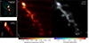 |
Fig. 2. Jet structure of 3C 279 revealed by RadioAstron. a: Total intensity (left) and linearly polarized (right) RadioAstron image at 22 GHz obtained on January 15, 2018. Both images show brightness temperature in color scale (afmhot and grayscale, respectively), though the image on the right also shows the recovered electric vector position angles overlaid as ticks. Their length and color are proportional to the level of linearly polarized intensity and fractional polarization, respectively. EHT aligned image from panel b is also displayed in contours over total intensity image. b: The EHT image at 230 GHz obtained in April 2017 at 1:1 scale and aligned to our RadioAstron image -in contours- using their respective pixel with maximum brightness. Contours are equally spaced in 7 levels within the data range. c: The 43 GHz close-in-time image from BEAM-ME program from Feurbary 2018. White ellipses at the bottom-left corners show the convolving beams. Bottom colour bars refer only to information displayed on a. |
The core region displays a bend toward the south of almost 90 degrees connecting with the rest of the straight emission, similar to the structure found in 2014. At around 1 mas from the core, the extended jet shows a gentle curve toward the southwest, coincident with the region where the filament was observed in 2014 but slightly farther away from the core (see also Fig. 3). No filamentary structure has been detected for our 2018 epoch. However, the similarities in structure hint toward the existence of a possibly more complex structure that does not show in this particular epoch, maybe due to the sparsity of the (u,v) coverage and the decrease in brightness of the source (see Sect. 3.3 for more detail).
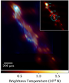 |
Fig. 3. Main image: Direct comparison between the 2014 and 2018 images of 3C 279 at 22 GHz with RadioAstron. The 2018 epoch is plotted in a warm color scale afmhot and aligned with the 2014 epoch (Fuentes et al. 2023), in blue, using the brightest pixel. The inset panel shows the Gaussian components from the model fitting process overlapped onto the image. The fifth component (E) is not shown since it is a large component that is necessary to take into account the diffuse emission. |
Figure 2 also allows us to study the polarized structure of the source. The EVPA direction (plotted as overlayed ticks that vary in length and color, which are proportional to the level of linearly polarized intensity and fractional polarization, respectively) appears to mostly follow the direction of the jet, suggesting that the magnetic field in the jet has a predominant toroidal component in the plane of the sky (relativistic effects are assumed not to strongly influence the perpendicular direction between electric and magnetic fields direction). At the core, EVPAs show a less organized distribution. As for the rest of the emission, it mostly shows an EVPA orientation parallel to the jet direction, as in 2014 observations (Fuentes et al. 2023) and therefore in agreement with a dominant toroidal magnetic field.
Figure 2 also shows BEAM-ME (43 GHz) close-in-time and EHT (230 GHz) 2017 observations at the bottom left and top left of the figure, respectively. The data from the monitoring program MOJAVE at 15 GHz are also available but too far apart in time (4-5 months) to be considered for this rapidly changing source.
When comparing our observations to the BEAM-ME VLBA data at 43 GHz from close-in-time observations, we could see that not only the general total intensity structure and jet direction remains the same with respect to the one we found but the polarization as well. EVPAs from 43 GHz are found to be oriented along the jet direction on parsec scales, indicating a magnetic field mainly perpendicular to the relativistic jet (Jorstad et al. 2005).
From the EHT image taken 9 months prior to our observations (Kim et al. 2020), we could see how the double structure found in the core fits consistently within the one we found (plotted in contours in the top-left panel). The core shift between both frequencies is ignored for the alignment, although it can be estimated as ∼40 μas. This particular alignment using the brightest pixel is motivated by the incompatible fields of view from EHT (230 GHz) and RadioAstron image (22 GHz). This is due to the different sensitivity to the extended structure between the two arrays as well as the fact that optically thin jet emission at 22 GHz will most likely be below the flux sensitivity at 230 GHz, even if it was sensitive to these spatial scales. Thus, it makes an alignment on optically thin components unfeasible.
3.1. Comparison with the 2014 results
Next, we look at a direct comparison between the previous RadioAstron observation of 3C 279 at 22 GHz from 2014 observations (Fuentes et al. 2023) and our 2018 data. A summary of the main differences is shown in Table 2. Fig. 3 shows both images overlayed in a ∼1.7 × 1.7 mas field of view, where the 2014 epoch is plotted in blue and aligned using the brightest pixel of both images.
Summary of the main differences between the 2014 and 2018 observations of 3C 279 at 22 GHz with RadioAstron.
The main difference observed in 2018 epoch is that the filamentary structure seen in Fuentes et al. (2023) (2014 epoch) does not appear to be present four years later in 2018. The orientation of the jet direction has also changed between both epochs, being slightly rotated in a counterclockwise motion.
The total intensity of the source has changed greatly, as mentioned in the previous subsection, going from 27.16 Jy in 2014 to 10.2 Jy in 2018. In 2014 observations, bright emission regions could be observed due to Doppler boosting. However, these features do not appear so clearly in the 2018 data. The integrated degree of linear polarization of the source is found to be around 5% in 2018, unlike the 10% found in 2014, hinting at more ordered magnetic fields. Nevertheless, from Fig. 2 it is possible to see that the EVPA direction (see Section 2) in 2018 is similar to that of the 2014 observations, still mostly parallel the jet direction, supporting the existence of a strong toroidal component and in agreement with a helical magnetic field configuration. In some regions, however, such as next to the core or at the bend by the end of the jet we detect, this general direction seems to rotate and become almost perpendicular to it. Our findings concur with previous detections of toroidal magnetic fields using VLBI polarimetric studies (e.g., Cho et al. 2024) through polarization structures and transverse Faraday rotation measure gradients (Toscano et al. 2025; Kovalev et al. 2025).
3.2. Gamma-ray flaring activity in 2018
As a very active and variable blazar, 3C 279 is also a powerful gamma-ray source and the first one showing strong and rapid variability at GeV energies (Hartman et al. 1992). It is also the first flat-spectrum radio quasar detected above 100 GeV (MAGIC Collaboration 2008).
After several high-energy flares in 2013 and 2015, 3C 279 became very active again in 2018, with fluxes exceeding the previous 2015 values. Several studies have been carried out on the January 2018 gamma-ray flare, focusing on the high-energy correlation between multi-wave bands with hour-binned light curves (Shah et al. 2019; Prince 2020; Goyal et al. 2022), on particle acceleration, or on the magnetic reconnection mechanism (Wang et al. 2022; Tolamatti et al. 2022).
The flare reached its peak on January 18, 2018 (Shukla & Mannheim 2020), three days after the RA observation. The peak of this flare went up to 4.0 ⋅ 10−5 ph cm−2 s−1, which corresponds to 0.0152 MeV/cm2/s (2.4 ⋅ 10−8 erg cm−2 s−1). The flare duration inferred as the FWHM of the fitted Gaussian is ∼6 days. This event can be compared to two previous major flares of 3C 279: the June 2015 flare, which peaked at (3.91 ± 0.25)⋅10−5 ph cm−2 s−1 (Paliya 2015) with sub-day variability, and the December 2013 flare (Paliya et al. 2016), characterized by extremely fast and intense sub-flares lasting only a few hours, with a very hard gamma-ray spectrum. While the 2018 flare reached a photon flux comparable to the 2015 event, its smoother and longer evolution stands in contrast to the shorter and more rapidly variable behavior seen in the 2013 and 2015 flares.
Our observations are quite close in time with respect to the gamma-ray flare detected in January 2018. In fact, according to the Fermi database, our observations took place while the flare was rising (Fig. 4). Based on multifrequency analysis presented in Mohana et al. (2023), the radio light curve of 3C 279 seems quite flat around the moment of our observations (both at 22 GHz and 43 GHz, as can be seen in Fig. 6), and does not show an increment in flux density until the end of 2020. Thus, the high values reported for the January 2018 gamma-ray flare do not show a visible impact or correlation with our observations, similar to the flares in 2013 and 2015, which also show no correlation with the radio band.
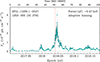 |
Fig. 4. Gamma-ray light curve of 3C 279 (positionally associated with 4FGL J1256.1-0547) constructed from Fermi-LAT data using adaptive binning (Lott et al. 2012) with a constant relative uncertainty on flux of ∼15% in each bin. The vertical red dashed line indicates the epoch of RadioAstron observations on January 15, 2018, which coincides with the rising phase of a prominent short-duration (6.8 days) flare reaching a peak of 4.0 ⋅ 10−5 ph cm−2 s−1 (2.4 ⋅ 10−8 erg cm−2 s−1) on January 18, 2018. |
3.3. Synthetic data
Previous observations from Fuentes et al. (2023) were able to detect a filamentary structure. Therefore, it is natural to ask whether the reason for the lack of detection of these filaments in our observations lies in the natural evolution of the source or elsewhere, such as the sparsity of the (u,v) coverage. To answer this question, we applied a methodology similar to the one used in Fuentes et al. (2023) and carried out tests using the same synthetic data model.
The synthetic data in Fig. 5 represent a couple of intertwined filaments forming a rotated-eight shape in a field of view of 1.3 × 1.3 mas. By using eht-imaging, we simulated observations of the ground-truth image under the same conditions of a certain observation. That is to say, using the same baselines, thermal noise, phase corruption, and gain uncertainties from the stations. In this case, we performed this test with data from two different (u,v) coverages: our epoch from January 15, 2018, at 22GHz and the BEAM-ME epoch from February 17, 2018, at 43 GHz; each is displayed in a different row. For all datasets, the same approach was used in the imaging reconstruction, namely, using either only closure quantities (closure phases and log closure amplitudes) or a combination of a first image with only closures and then performing self-calibration and adding complex visibilities.
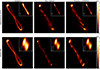 |
Fig. 5. Synthetic data test using different data terms to probe filament detection using the RadioAstron (u,v)-coverage of 2018 (first row) and BEAM-ME February 2018 (second row). Main images have a field of view of 1.1 × 1.1 mas, while miniatures at the top right show the main images convolved with its respective nominal beams on a field of view of 1.3 × 1.3 mas and 2 × 2 mas, for each row respectively. Units of the color wedges indicate brightness temperature in Kelvin. The nominal beam for each dataset is plotted in white at the bottom left of the miniature images. |
In Fig. 5, in the first row, we show the results with our RadioAstron data. When using only closure quantities, the reconstruction takes the shape of a roughly straight line in the right direction but shows no sign of filaments. When adding visibilities, the reconstruction marginally improves, but it is still not possible to discern any loops. However, it is possible to detect the two brightest features at both ends of the loops, though not the one where the filaments intersect. Thus, even if filaments were present in the source at the time of our observations, their existence could not be reliably confirmed.
For the second row, where the BEAM-ME synthetic test is displayed, we also tried to see if it would be possible to recover the filamentary structure with the coverage of this monitoring program. Again, as can be observed in Fig. 5 (lower panel), it is not possible to recover any filaments, but there is an approximately straight line of emission that also shows an uneven brightness distribution. The reconstruction does not really improve when adding the visibilities, as happened in the previous case, but it does manage to obtain the bright features at the loop edges. A successful recovery of the filamentary structure can be seen in the test performed in Fuentes et al. (2023), thus supporting their existence.
3.4. 43 GHz VLBA BEAM-ME evolution
We can contextualize our results by looking at public data from BEAM-ME at 43 GHz and thus study the brightness evolution of the 3C 279 jet and its dynamic nature. In Fig. 7, we show epochs yearly across approximately four years, from 2014 to 2018, in order to discern any change in the source that may confirm and help elucidate the lack of filament detection.
On the BEAM-ME webpage, these images made by Difmap using the traditional CLEAN method are readily accessible, but we used the already calibrated fits files and displayed them (not reconstructed) in Stokes I using eht-imaging library, the same library used to reconstruct the 2018 RadioAstron data. By doing so, we captured a comprehensive view of the temporal evolution of the blazar over four years and observed that this period in particular highlights a “turning off” phase.
We note that from 2014 to 2018, the source progressively decreased its brightness. This fact is also clear when looking at the light curve shown in Fig. 6. This decline in brightness is not uncommon in blazars known for the variability of their light curves, often on timescales of years to decades (e.g., Teräsranta et al. 1992; Lister et al. 2018; Mohana et al. 2023; Eppel et al. 2024). Such variability can be influenced by changes in the Doppler beaming factor or the accretion rate onto the black hole.
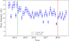 |
Fig. 6. Light curve of 3C 279 at 43 GHz VLBA from the BEAM-ME project constructed using the flux density of CLEAN images (within a field of view of 2 × 2 mas). The red line indicates the observations from 2018, and the green line is for those from 2014. We estimated data uncertainties of 10%, indicated with error bars. |
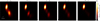 |
Fig. 7. BEAM-ME 43 GHz VLBA yearly evolution using public data between 2014 and 2018 of 3C 279 using a field of view of 2 × 2 mas. |
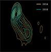 |
Fig. 8. BEAM-ME image comparison between epochs from 2014 and 2018. Contours display 0.2 to 0.9 of the maximum brightness in intervals of 0.1. |
Notably, the decrease in brightness of the source poses significant implications for our ability to observe and resolve any structural details in the jet, both in total intensity and polarization. This means that as the source dims toward 2018, features in the jet become harder to detect and any structure is substituted by a mostly straight faint line of emission, impeding the study of the intricate magnetic field configurations and plasma dynamics that drive the jet physics in 3C 279.
Moreover, we can directly compare BEAM-ME images from close-in-time epochs to the RadioAstron observations, i.e., from February 2014 and 2018 (see Fig. 8). It is possible to see a slight change in the orientation, with the 2018 epoch showing a small counterclockwise direction. This behavior is also observed between the RadioAstron epochs (see Sect. 3.1).
3.5. Brightness temperature
The plasma acceleration and radiative evolution of the jet’s innermost region can be studied through estimations of the brightness temperature (Readhead 1994; Marscher 1995; Kovalev et al. 2005; Fromm et al. 2013; Röder et al. 2025). It mainly provides an approximation of the source brightness, making it possible to characterize the energy partition between plasma and the magnetic field when assuming self-absorbed synchrotron radiation (Readhead 1994; Homan et al. 2006; Kovalev et al. 2016; Homan et al. 2021).
The inverse Compton process limits the maximum intrinsic brightness temperature for incoherent synchrotron sources, corresponding to (0.3–1)×1012 K (Kellermann & Pauliny-Toth 1969). If a flare has taken place and the brightness temperature exceeds this limit, the source is expected to cool rapidly – on the order of a day – due to catastrophic inverse Compton losses. This estimate assumes a homogeneous, self-absorbed synchrotron source with no significant Doppler boosting, no ongoing particle acceleration, and efficient energy loss via inverse Compton scattering (e.g., Readhead 1994; Slysh 1992). Complimentary to this, another upper threshold arises for sources near the equipartition, referred to as equipartition brightness temperature (Teq, where the energy density of the magnetic field is approximately equal to the energy density of the relativistic particles), of value ∼5 × 10¹⁰ K (Readhead 1994; Singal 2009).
Refractive scattering in the interstellar medium can introduce substructure that biases brightness temperature estimates at longer wavelengths (Johnson et al. 2016), but its impact decreases sharply with frequency. At 22 GHz this effect is negligible and therefore not taken into account in the following analysis.
The brightness temperature parameter is commonly determined by modeling the structure of the emitting region through the flux density and angular size of the model components. The observed brightness temperature in this work was calculated by fitting the circular Gaussian components with different flux densities and sizes (see Table 3 columns 1 to 5 and Fig. 3) using the modelfit function in Difmap (Pushkarev & Kovalev 2012; Gómez et al. 2022). The error for the flux density was estimated to be ∼10% since it is mostly dominated by the a priori calibration. Errors for the rest of the quantities were also set to ∼10% of their value since the statistical errors from the fitting itself are commonly misleadingly small and do not convey the systematic uncertainties from the measurements. The brightness temperature is given by (e.g., Gómez et al. 2022)
Model fitting results from the RadioAstron image.
![Mathematical equation: $$ \begin{aligned} T_{\rm {b,obs}}=1.22 \times 10^{12} \left( \frac{S_{\nu }}{\text{ Jy}} \right) \left(\frac{\nu _{\rm {obs}}}{\text{ GHz}}\right)^{-2} \left(\frac{\theta _{\rm {obs}}}{\text{ mas}}\right)^{-2} \, [K]\,, \end{aligned} $$](/articles/aa/full_html/2025/12/aa55188-25/aa55188-25-eq3.gif) (2)
(2)
where Sν is the component flux density, θobs is the size of the model component, and νobs is the observing frequency.
Using Eq. (2), we estimated the brightness temperatures corresponding to the different components of the image model (see Table 3, column 6), finding five different components that amount to 10.0 Jy (out of the 10.2 Jy found in the image), which is a good approximation. In order to get a good fit, a large component, E, is required to capture some extended emission (as seen in Table 3), but it is not shown in Fig. 3.
Moreover, to calculate the intrinsic brightness temperature of the jet, we also needed to take into account the cosmological correction and the Doppler boosting effect. The blazar 3C 279, with an estimated viewing angle of θ ∼ 2° (Jorstad et al. 2017), is known to have a wide range of Doppler factor (δ) values [10–40] (Jorstad et al. 2005; Bloom et al. 2013; Jorstad et al. 2017; Kim et al. 2020). The observed brightness temperature is related to the intrinsic one of the jet, Tb, int, as follows:
 (3)
(3)
where z is the cosmological redshift of the source.
From the observed brightness temperature values found, assuming the most likely scenario that the radiative losses are from synchrotron radiation, we could see that the observed brightness temperature of the core has a value of 1.6 × 10¹² K. Such a high and even higher values are common in RadioAstron observations (e.g., Kovalev et al. 2016; Gómez et al. 2016; Bruni et al. 2017; Pilipenko et al. 2017; Kovalev et al. 2020; Röder et al. 2025).
However, the intrinsic brightness temperature value of the core, of ∼ 1011 K, calculated assuming a Doppler factor of 24 (Jorstad et al. 2005; Kim et al. 2020), can be reconciled with the Inverse Compton limit when considering the high Doppler factor observed in 3C 279. This value suggests that the core is close to equipartition, meaning that the energy densities of the relativistic particles and the magnetic field are nearly balanced. This is consistent with the lack of evident flaring events in radio frequencies around the time of our observations. The rest of the components show a decrease of brightness temperature when moving farther away from the core, following the expected energy dissipation with distance via adiabatic and radiative losses.
The observed brightness temperature at the core (including cosmological and Doppler boosting corrections), where the frequency is also affected by Doppler factor so that νint = νobs(1 + z)/δ, can be related to the magnetic field strength of a synchrotron self-absorbed core (Section 5.3 of Condon & Ransom 2016). We can justify the core to be optically thick by establishing a rough spectral index (α) comparing the brightness of the 22 GHz RadioAstron core (6.40 Jy) to that of the BEAM-ME 43 GHz core (8.85 Jy, calculated also using modelfit), yielding a value of ∼0.48. This result is consistent with optically thick synchrotron emission from a stratified AGN jet core, which typically falls between (0.2–0.6). Therefore, we could apply the following relation to the magnetic field:
![Mathematical equation: $$ \begin{aligned} B = 1.4 \times 10^{21} \left(\frac{\nu _{\text{obs}}}{\text{ GHz}}\right) \left(\frac{T_{\rm {b,obs}} }{\text{ K}}\right)^{-2} \frac{\delta }{(1+z)} \ \text{[G]}\,, \end{aligned} $$](/articles/aa/full_html/2025/12/aa55188-25/aa55188-25-eq5.gif) (4)
(4)
yielding a magnetic field strength of ∼0.2 G near the core. This value is consistent with those found in Röder et al. (2025), based on Kovalev et al. (in prep.).
4. Conclusions
We carried out RadioAstron observations of 3C 279 on January 15, 2018, at 22 GHz, representing the last possible observations of this source with this space VLBI mission. The array sensitivity together with RML methods (eht-imaging) enabled us to obtain super-resolved images of the 3C 279 jet with a high angular resolution (26 μ as). The images revealed the lack of detection of a filament-like structure found in a similar previous study with RadioAstron using data from a 2014 epoch (Fuentes et al. 2023).
Analysis using synthetic data with both our array properties and those of BEAM-ME close-in-time, supports the fact that the lack of filament detection is not necessarily related to their non-existence, but most likely due to insufficient (u,v) coverage. Moreover, observations from BEAM-ME public data revealed that over the 4-year period 2014–2018, the source exhibited a gradual decline in brightness, which affected our ability to resolve its jet structure in both total intensity and polarization.
We also explored the gamma-ray emission relation with our observations, finding that our observations coincide with the rising of a gamma-ray flare that surpasses the previous flare from 2015 in brightness. Nevertheless, we find that this phenomenon does not seem to impact or correlate with our results.
Finally, a study of the brightness temperature using model fitting with Gaussian components yielded a core with an observed brightness temperature of the order of 1012 K, in agreement with previous RadioAstron observations, and an estimated magnetic field strength of ∼0.2 G in the core region. The values found for the jet’s brightness temperature suggest it to be close to equipartition, as can be expected for a source in a low activity period.
Data availability
The reduced images are available at the CDS via https://cdsarc.cds.unistra.fr/viz-bin/cat/J/A+A/704/A225
Acknowledgments
The authors thank anonymous referee for their useful comments and suggestions that helped to improve this manuscript. The work at the IAA-CSIC is supported in part by the Spanish Ministerio de Economía y Competitividad (PID2022-140888NB-C21), the Ramón y Cajal grant RYC2023-042988-I from the Spanish Ministry of Science and Innovation, the Consejo Superior de Investigaciones Científicas (grant 2019AEP112), and the State Agency for Research of the Spanish MCIU through the “Center of Excellence Severo Ochoa” grant CEX2021-001131-S funded by MCIN/AEI/10.13039/501100011033 awarded to the Instituto de Astrofísica de Andalucía. LIG gratefully acknowledges support by the Chinese Academy of Sciences PIFI program, grant No. 2024PVA0008. YYK was supported by the MuSES project, which has received funding from the European Union (ERC grant agreement No 101142396). Views and opinions expressed are however those of the author(s) only and do not necessarily reflect those of the European Union or ERCEA. Neither the European Union nor the granting authority can be held responsible for them. RadioAstron, a project led by the Astro Space Center of the Lebedev Physical Institute of the Russian Academy of Sciences and the Lavochkin Scientific and Production Association under a contract with the Russian Federal Space Agency, in collaboration with partner organizations in Russia and other countries. The European VLBI Network, a joint facility of independent European, African, Asian, and North American radio astronomy institutes. Scientific results from data presented in this publication are derived from the EVN project. This research is partly based on observations with the 100m telescope of the MPIfR at Effelsberg. This publication makes use of data obtained at Metsähovi cby Aalto University in Finland. The Long Baseline Array is part of the Australia Telescope National Facility (https://ror.org/05qajvd42) which is funded by the Australian Government for operation as a National Facility managed by CSIRO. Special thanks go to the people designing and supporting the space and ground observations. This research is based on observations correlated at the Bonn Correlator modified for RadioAstron correlation, jointly operated by the Max-Planck-Institut für Radioastronomie, and the Federal Agency for Cartography and Geodesy. This study makes use of 43 GHz VLBA data from the VLBA-BU Blazar Monitoring Program (VLBA-BU-BLAZAR; http://www.bu.edu/blazars/BEAM-ME.html), funded by NASA through Fermi Guest Investigator grant number 80NSSC20K1567.
References
- Blandford, R. D., & Payne, D. G. 1982, MNRAS, 199, 883 [CrossRef] [Google Scholar]
- Blandford, R. D., & Znajek, R. L. 1977, MNRAS, 179, 433 [NASA ADS] [CrossRef] [Google Scholar]
- Blandford, R., Meier, D., & Readhead, A. 2019, ARA&A, 57, 467 [NASA ADS] [CrossRef] [Google Scholar]
- Bloom, S. D., Fromm, C. M., & Ros, E. 2013, AJ, 145, 12 [Google Scholar]
- Boccardi, B., Krichbaum, T. P., Ros, E., & Zensus, J. A. 2017, A&A Rev., 25, 4 [NASA ADS] [CrossRef] [Google Scholar]
- Bruni, G., Anderson, J. M., Alef, W., et al. 2016, Galaxies, 4, 55 [Google Scholar]
- Bruni, G., Gómez, J. L., Casadio, C., et al. 2017, A&A, 604, A111 [NASA ADS] [CrossRef] [EDP Sciences] [Google Scholar]
- Bruni, G., Gómez, J. L., Vega-García, L., et al. 2021, A&A, 654, A27 [NASA ADS] [CrossRef] [EDP Sciences] [Google Scholar]
- Chael, A. A., Johnson, M. D., Narayan, R., et al. 2016, ApJ, 829, 11 [Google Scholar]
- Chael, A. A., Johnson, M. D., Bouman, K. L., et al. 2018, ApJ, 857, 23 [Google Scholar]
- Cho, I., Gómez, J. L., Lico, R., et al. 2024, A&A, 683, A248 [NASA ADS] [CrossRef] [EDP Sciences] [Google Scholar]
- Cohen, M. H., Cannon, W., Purcell, G. H., et al. 1971, ApJ, 170, 207 [NASA ADS] [CrossRef] [Google Scholar]
- Condon, J. J., & Ransom, S. M. 2016, Essential Radio Astronomy (Princeton University Press) [Google Scholar]
- de Pater, I., & Perley, R. A. 1983, ApJ, 273, 64 [Google Scholar]
- EHTC, (Akiyama, K., et al.) 2019a, ApJ, 875, L1 [NASA ADS] [CrossRef] [Google Scholar]
- EHTC, (Akiyama, K., et al.) 2019b, ApJ, 875, L4 [CrossRef] [Google Scholar]
- EHTC, (Akiyama, K., et al.) 2021, ApJ, 910, L12 [CrossRef] [Google Scholar]
- EHTC, (Akiyama, K., et al.) 2022a, ApJ, 930, L12 [NASA ADS] [CrossRef] [Google Scholar]
- EHTC, (Akiyama, K., et al.) 2022b, ApJ, 930, L14 [NASA ADS] [CrossRef] [Google Scholar]
- EHTC, (Akiyama, K., et al.) 2024, ApJ, 964, L25 [NASA ADS] [CrossRef] [Google Scholar]
- Eppel, F., Kadler, M., Heßdörfer, J., et al. 2024, A&A, 684, A11 [NASA ADS] [CrossRef] [EDP Sciences] [Google Scholar]
- Fromm, C. M., Ros, E., Perucho, M., et al. 2013, A&A, 557, A105 [NASA ADS] [CrossRef] [EDP Sciences] [Google Scholar]
- Fuentes, A., Gómez, J. L., Martí, J. M., et al. 2023, Nat. Astron., 7, 1359 [NASA ADS] [CrossRef] [Google Scholar]
- Gabuzda, D. C. 2021, Galaxies, 9, 58 [NASA ADS] [CrossRef] [Google Scholar]
- Giovannini, G., Savolainen, T., Orienti, M., et al. 2018, Nat. Astron., 2, 472 [Google Scholar]
- Gómez, J. L., Marscher, A. P., Alberdi, A., Jorstad, S. G., & Agudo, I. 2001, ApJ, 561, L161 [NASA ADS] [CrossRef] [Google Scholar]
- Gómez, J. L., Lobanov, A. P., Bruni, G., et al. 2016, ApJ, 817, 96 [Google Scholar]
- Gómez, J. L., Traianou, E., Krichbaum, T. P., et al. 2022, ApJ, 924, 122 [Google Scholar]
- Goyal, A., Soida, M., Stawarz, Ł., et al. 2022, ApJ, 927, 214 [CrossRef] [Google Scholar]
- Greisen, E. W. 2003, in Information Handling in Astronomy - Historical Vistas, ed. A. Heck, Astrophys. Space Sci. Lib., 285, 109 [NASA ADS] [CrossRef] [Google Scholar]
- Hartman, R. C., Bertsch, D. L., Fichtel, C. E., et al. 1992, ApJ, 385, L1 [Google Scholar]
- Högbom, J. A. 1974, A&AS, 15, 417 [Google Scholar]
- Homan, D. C., Lister, M. L., Kellermann, K. I., et al. 2003, ApJ, 589, L9 [Google Scholar]
- Homan, D. C., Kovalev, Y. Y., Lister, M. L., et al. 2006, ApJ, 642, L115 [NASA ADS] [CrossRef] [Google Scholar]
- Homan, D. C., Cohen, M. H., Hovatta, T., et al. 2021, ApJ, 923, 67 [NASA ADS] [CrossRef] [Google Scholar]
- Johnson, M. D., Kovalev, Y. Y., Gwinn, C. R., et al. 2016, ApJ, 820, L10 [Google Scholar]
- Jorstad, S. G., Marscher, A. P., Lister, M. L., et al. 2005, AJ, 130, 1418 [Google Scholar]
- Jorstad, S. G., Marscher, A. P., Morozova, D. A., et al. 2017, ApJ, 846, 98 [Google Scholar]
- Kardashev, N. S., Khartov, V. V., Abramov, V. V., et al. 2013, Astron. Rep., 57, 153 [Google Scholar]
- Kellermann, K. I., & Pauliny-Toth, I. I. K. 1969, ApJ, 155, L71 [NASA ADS] [CrossRef] [Google Scholar]
- Kettenis, M., van Langevelde, H. J., Reynolds, C., & Cotton, B. 2006, in Astronomical Data Analysis Software and Systems XV, eds. C. Gabriel, D. Arviset, D. Ponz, & S. Enrique, ASP Conf. Ser., 351, 497 [NASA ADS] [Google Scholar]
- Kim, J. Y., Krichbaum, T. P., Broderick, A. E., et al. 2020, A&A, 640, A69 [NASA ADS] [CrossRef] [EDP Sciences] [Google Scholar]
- Knight, C. A., Robertson, D. S., Rogers, A. E. E., et al. 1971, Science, 172, 52 [Google Scholar]
- Kovalev, Y. Y., Kellermann, K. I., Lister, M. L., et al. 2005, AJ, 130, 2473 [Google Scholar]
- Kovalev, Y. Y., Kardashev, N. S., Kellermann, K. I., et al. 2016, ApJ, 820, L9 [Google Scholar]
- Kovalev, Y. Y., Kardashev, N. S., Sokolovsky, K. V., et al. 2020, Adv. Space Res., 65, 705 [Google Scholar]
- Kovalev, Y. Y., Pushkarev, A. B., Gómez, J. L., et al. 2025, A&A, 700, L12 [NASA ADS] [CrossRef] [EDP Sciences] [Google Scholar]
- Lister, M. L., Aller, M. F., Aller, H. D., et al. 2018, ApJS, 234, 12 [CrossRef] [Google Scholar]
- Lister, M. L., Homan, D. C., Hovatta, T., et al. 2019, ApJ, 874, 43 [NASA ADS] [CrossRef] [Google Scholar]
- Lister, M. L., Homan, D. C., Kellermann, K. I., et al. 2021, ApJ, 923, 30 [NASA ADS] [CrossRef] [Google Scholar]
- Lobanov, A. 2015, A&A, 574, A84 [NASA ADS] [CrossRef] [EDP Sciences] [Google Scholar]
- Lobanov, A. P., Gómez, J. L., Bruni, G., et al. 2015, A&A, 583, A100 [EDP Sciences] [Google Scholar]
- Lott, B., Escande, L., Larsson, S., & Ballet, J. 2012, A&A, 544, A6 [NASA ADS] [CrossRef] [EDP Sciences] [Google Scholar]
- MAGIC Collaboration (Albert, J., et al.) 2008, Science, 320, 1752 [NASA ADS] [CrossRef] [Google Scholar]
- Marscher, A. P. 1995, Proc. Nat. Acad. Sci., 92, 11439 [NASA ADS] [CrossRef] [Google Scholar]
- Marziani, P., Sulentic, J. W., Dultzin-Hacyan, D., Calvani, M., & Moles, M. 1996, ApJS, 104, 37 [Google Scholar]
- Mohana, K., Gupta, A. C., Marscher, A. P., et al. 2023, MNRAS, 527, 6970 [Google Scholar]
- Paliya, V. S. 2015, ApJ, 808, L48 [Google Scholar]
- Paliya, V. S., Diltz, C., Böttcher, M., Stalin, C. S., & Buckley, D. 2016, ApJ, 817, 61 [Google Scholar]
- Pilipenko, S. V., Kovalev, Y. Y., Andrianov, A. S., et al. 2017, MNRAS, 474, 3523 [Google Scholar]
- Popkov, A. V., Kovalev, Y. Y., Petrov, L. Y., & Kovalev, Y. A. 2021, AJ, 161, 88 [CrossRef] [Google Scholar]
- Prince, R. 2020, ApJ, 890, 164 [NASA ADS] [CrossRef] [Google Scholar]
- Pushkarev, A. B., & Kovalev, Y. Y. 2012, A&A, 544, A34 [NASA ADS] [CrossRef] [EDP Sciences] [Google Scholar]
- Pushkarev, A. B., Aller, H. D., Aller, M. F., et al. 2023, MNRAS, 520, 6053 [NASA ADS] [CrossRef] [Google Scholar]
- Readhead, A. C. S. 1994, ApJ, 426, 51 [Google Scholar]
- Röder, J., Wielgus, M., Lobanov, A. P., et al. 2025, A&A, 695, A233 [NASA ADS] [CrossRef] [EDP Sciences] [Google Scholar]
- Savolainen, T., Giovannini, G., Kovalev, Y. Y., et al. 2023, A&A, 676, A114 [NASA ADS] [CrossRef] [EDP Sciences] [Google Scholar]
- Shah, Z., Jithesh, V., Sahayanathan, S., Misra, R., & Iqbal, N. 2019, MNRAS, 484, 3168 [Google Scholar]
- Shepherd, M. 2011, Difmap: Synthesis Imaging of Visibility Data, Astrophysics Source Code Library [record ascl:1103.001] [Google Scholar]
- Shepherd, M. C., Pearson, T. J., & Taylor, G. B. 1994, BAAS, 26, 987 [NASA ADS] [Google Scholar]
- Shepherd, M. C., Pearson, T. J., & Taylor, G. B. 1995, Bull. Astron. Soc., 27, 903 [Google Scholar]
- Shukla, A., & Mannheim, K. 2020, Nat. Commun., 11, 4176 [NASA ADS] [CrossRef] [Google Scholar]
- Singal, A. K. 2009, ApJ, 703, L109 [NASA ADS] [CrossRef] [Google Scholar]
- Slysh, V. I. 1992, ApJ, 391, 453 [Google Scholar]
- Teräsranta, H., Tornikoski, M., Karlamaa, K., et al. 1992, Proceedings of The Variability of Blazars (United Kingdom: Cambridge University Press), 159 [Google Scholar]
- Tolamatti, A., Ghosal, B., Singh, K., et al. 2022, Astropart. Phys., 139, 102687 [Google Scholar]
- Toscano, Molina, S. N., Gomez, J. L., et al. 2025, A&A, 698, A210 [Google Scholar]
- Traianou, E., Gómez, J. L., Cho, I., et al. 2025, A&A, 700, A16 [NASA ADS] [CrossRef] [EDP Sciences] [Google Scholar]
- Vega-García, L., Lobanov, A. P., Perucho, M., et al. 2020, A&A, 641, A40 [NASA ADS] [CrossRef] [EDP Sciences] [Google Scholar]
- Wang, G., Fan, J., Xiao, H., & Cai, J. 2022, PASP, 134, 104101 [Google Scholar]
- Weaver, Z. R., Jorstad, S. G., Marscher, A. P., et al. 2022, ApJS, 260, 12 [NASA ADS] [CrossRef] [Google Scholar]
- Whitney, A. R., Shapiro, I. I., Rogers, A. E. E., et al. 1971, Science, 173, 225 [NASA ADS] [CrossRef] [Google Scholar]
Appendix A: Difmap model image
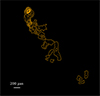 |
Fig. A.1. CLEAN model in contours of 3C 279 RadioAstron 2018 observations using Difmap and plotted using a Python script. Contours are plotted at levels of 0.1 to 0.9 times the peak brightness, in steps of 0.1. |
Appendix B: Parameter survey
To ensure a robust reconstruction regardless of the regularizers used in the imaging process, we perform an additional parameter survey. The values selected survey over lower values of “mem” parameter, testing the impact of the prior image resemblance, and higher values for ’tv’ and ’l1’, checking that neither the regularizers enhancing smoothness or compactness, respectively, cause any major structural changes in the final reconstruction.
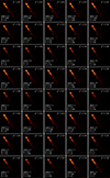 |
Fig. B.1. Parameter survey of 3C 279 RadioAstron 2018 displaying similar morphology. Visibilities χ2 values are at the top right of each image, and the regularizer combination at the bottom left. |
All Tables
Summary of the main differences between the 2014 and 2018 observations of 3C 279 at 22 GHz with RadioAstron.
All Figures
|
Fig. 1. Coverage in the (u,v) plane of the fringe-fitted interferometric visibilities of 3C 279 observed by RadioAstron at 22 GHz on January 15, 2018. The top panel shows only the ground baselines, while the bottom panel shows all baselines, with those of RadioAstron in gray. |
| In the text | |
|
Fig. 2. Jet structure of 3C 279 revealed by RadioAstron. a: Total intensity (left) and linearly polarized (right) RadioAstron image at 22 GHz obtained on January 15, 2018. Both images show brightness temperature in color scale (afmhot and grayscale, respectively), though the image on the right also shows the recovered electric vector position angles overlaid as ticks. Their length and color are proportional to the level of linearly polarized intensity and fractional polarization, respectively. EHT aligned image from panel b is also displayed in contours over total intensity image. b: The EHT image at 230 GHz obtained in April 2017 at 1:1 scale and aligned to our RadioAstron image -in contours- using their respective pixel with maximum brightness. Contours are equally spaced in 7 levels within the data range. c: The 43 GHz close-in-time image from BEAM-ME program from Feurbary 2018. White ellipses at the bottom-left corners show the convolving beams. Bottom colour bars refer only to information displayed on a. |
| In the text | |
|
Fig. 3. Main image: Direct comparison between the 2014 and 2018 images of 3C 279 at 22 GHz with RadioAstron. The 2018 epoch is plotted in a warm color scale afmhot and aligned with the 2014 epoch (Fuentes et al. 2023), in blue, using the brightest pixel. The inset panel shows the Gaussian components from the model fitting process overlapped onto the image. The fifth component (E) is not shown since it is a large component that is necessary to take into account the diffuse emission. |
| In the text | |
|
Fig. 4. Gamma-ray light curve of 3C 279 (positionally associated with 4FGL J1256.1-0547) constructed from Fermi-LAT data using adaptive binning (Lott et al. 2012) with a constant relative uncertainty on flux of ∼15% in each bin. The vertical red dashed line indicates the epoch of RadioAstron observations on January 15, 2018, which coincides with the rising phase of a prominent short-duration (6.8 days) flare reaching a peak of 4.0 ⋅ 10−5 ph cm−2 s−1 (2.4 ⋅ 10−8 erg cm−2 s−1) on January 18, 2018. |
| In the text | |
|
Fig. 5. Synthetic data test using different data terms to probe filament detection using the RadioAstron (u,v)-coverage of 2018 (first row) and BEAM-ME February 2018 (second row). Main images have a field of view of 1.1 × 1.1 mas, while miniatures at the top right show the main images convolved with its respective nominal beams on a field of view of 1.3 × 1.3 mas and 2 × 2 mas, for each row respectively. Units of the color wedges indicate brightness temperature in Kelvin. The nominal beam for each dataset is plotted in white at the bottom left of the miniature images. |
| In the text | |
|
Fig. 6. Light curve of 3C 279 at 43 GHz VLBA from the BEAM-ME project constructed using the flux density of CLEAN images (within a field of view of 2 × 2 mas). The red line indicates the observations from 2018, and the green line is for those from 2014. We estimated data uncertainties of 10%, indicated with error bars. |
| In the text | |
|
Fig. 7. BEAM-ME 43 GHz VLBA yearly evolution using public data between 2014 and 2018 of 3C 279 using a field of view of 2 × 2 mas. |
| In the text | |
|
Fig. 8. BEAM-ME image comparison between epochs from 2014 and 2018. Contours display 0.2 to 0.9 of the maximum brightness in intervals of 0.1. |
| In the text | |
|
Fig. A.1. CLEAN model in contours of 3C 279 RadioAstron 2018 observations using Difmap and plotted using a Python script. Contours are plotted at levels of 0.1 to 0.9 times the peak brightness, in steps of 0.1. |
| In the text | |
|
Fig. B.1. Parameter survey of 3C 279 RadioAstron 2018 displaying similar morphology. Visibilities χ2 values are at the top right of each image, and the regularizer combination at the bottom left. |
| In the text | |
Current usage metrics show cumulative count of Article Views (full-text article views including HTML views, PDF and ePub downloads, according to the available data) and Abstracts Views on Vision4Press platform.
Data correspond to usage on the plateform after 2015. The current usage metrics is available 48-96 hours after online publication and is updated daily on week days.
Initial download of the metrics may take a while.