| Issue |
A&A
Volume 704, December 2025
|
|
|---|---|---|
| Article Number | A230 | |
| Number of page(s) | 11 | |
| Section | Stellar structure and evolution | |
| DOI | https://doi.org/10.1051/0004-6361/202555537 | |
| Published online | 16 December 2025 | |
Impact of near-degeneracy effects on linear rotational inversions for red giant stars
1
Heidelberger Institut für Theoretische Studien, Schloss-Wolfsbrunnenweg 35, 69118 Heidelberg, Germany
2
Institute for Astronomy, University of Hawai’i, 2680 Woodlawn Drive, Honolulu, HI 96822, USA
3
Department of Astronomy, Yale University, New Haven, CT 06520, USA
4
Max-Planck-Institut für Astrophysik, Karl-Schwarzschild-Straße 1, 85748 Garching, Germany
5
Center for Astronomy (ZAH/LSW), Heidelberg University, Königstuhl 12, 69117 Heidelberg, Germany
★ Corresponding author: This email address is being protected from spambots. You need JavaScript enabled to view it.
Received:
16
May
2025
Accepted:
29
September
2025
Abstract
Context.Accurate estimates of internal red giant rotation rates are crucial for constraining and improving current models of stellar rotation. Asteroseismic rotational inversions provide a means of estimating these internal rotation rates.
Aims. In this work, we focus on the observed differences in the rotationally induced frequency shifts between prograde and retrograde modes. These effects have been overlooked in previous studies estimating internal rotation rates of red giants using inversions. We systematically study the limits of applicability of linear rotational inversions as a function of the evolution on the red giant branch and of the underlying rotation rates.
Methods. We determine oscillation mode frequencies in the presence of rotation using the lowest-order perturbative approach and describe the differences between prograde and retrograde modes arising from the coupling of multiple mixed modes, also known as near-degeneracy effects. We computed synthetic rotational splittings, taking these near-degeneracy effects into account. We used red giant models with one solar mass, a large frequency separation between 16 and 9 μHz, and core rotation rates between 500 and 1500 nHz, covering the regime of observed parameters of Kepler red giant stars. Finally, we used these synthetic data to quantify the systematic errors in the internal rotation rates estimated by means of rotational inversions in the presence of near-degeneracy effects.
Results. We show that the systematic errors in the estimated rotation rates introduced by near-degeneracy effects surpass the observational uncertainties for more evolved and faster-rotating stars. For a core rotation rate of 500 nHz, linear inversions remain applicable over the range of models considered here, while for a core rotation rate of 1000 nHz, systematic errors become significant below a large frequency separation of 13 μHz.
Conclusions. The estimated rotation rates of some previously analysed red giants suffer from significant systematic errors that have not yet been accounted for. Nonetheless, reliable analyses with existing inversion methods are feasible for a number of red giants, and we expect there to be unexplored targets within the parameter ranges determined here. Finally, exploiting the observational potential of near-degeneracy effects is an important step towards obtaining more accurate estimates of internal red-giant rotation rates.
Key words: asteroseismology / stars: interiors / stars: oscillations / stars: rotation
NASA Hubble Fellow.
© The Authors 2025
 Open Access article, published by EDP Sciences, under the terms of the Creative Commons Attribution License (https://creativecommons.org/licenses/by/4.0), which permits unrestricted use, distribution, and reproduction in any medium, provided the original work is properly cited.
This article is published in open access under the Subscribe to Open model. This email address is being protected from spambots. You need JavaScript enabled to view it. to support open access publication.
1. Introduction
Stellar oscillations provide insights into the interiors of stars through a collection of methods known as ‘inversions’ which probe their internal structure, magnetic field strength, and rotation. These inversion techniques aim to measure perturbations of the stellar structure (e.g. due to rotation) relative to a known fiducial state. The application of these methods requires several assumptions. Most notably, the use of linear inversions requires a linear relation to exist between the perturbation of the frequencies and the size of the perturbation. However, for rotational inversions of red giant stars, we may enter a regime in which this assumption of linearity is no longer valid (Deheuvels et al. 2017; Li et al. 2024).
Rotation is an important, yet poorly understood, property of stellar interiors. Rotation-induced chemical mixing can significantly alter the distribution of chemical elements within the star, for example, by increasing the supply of elements available for nuclear reactions in the core (e.g. Eggenberger et al. 2010). This may also alter the surface abundances measured through classical spectroscopy. Additionally, rotation also directly perturbs the structure of the star. Rapid rotation can modify the hydrostatic equilibrium (e.g. Maeder 2009) or the properties of convective motions, depending on the ratio of convective to rotational velocities (e.g. Käpylä 2024). Despite its importance, there is no conclusive description of the interplay between rotation and stellar evolution. Observations of internal rotation rates (Mosser et al. 2012; Gehan et al. 2018; Aerts et al. 2019; Li et al. 2024) indicate that an efficient mechanism must exist that transports angular momentum from the core to the envelope as stars evolve up the red giant branch (RGB) (e.g. Eggenberger et al. 2012, 2017; Ceillier et al. 2013; Marques et al. 2013; Spada et al. 2016). Several mechanisms have been suggested to explain this angular momentum transport, including hydrodynamical instabilities (Maeder 2009), internal gravity waves (Alvan et al. 2013; Fuller et al. 2014; Pinçon et al. 2017), mixed modes (Belkacem et al. 2015a,b; Bordadágua et al. 2025), and magnetic fields (Spruit 2002; Cantiello et al. 2014; Fuller et al. 2019; Eggenberger et al. 2019; Takahashi & Langer 2021). However, none are able to fully explain the rotational evolution along the RGB. Accurate measurement of internal rotation rates of red giants is therefore essential for testing and constraining stellar evolution models.
As in the Sun, global oscillations in red giants are stochastically driven by turbulent convection in the outer layers of the star. This excitation mechanism drives both radial and non-radial oscillations over multiple overtones, allowing us to probe the internal structure of these stars. In red giants, we also observe mixed modes – modes with a gravity (g-mode) character in the core and a pressure (p-mode) character in the outer layers of the star. Observation of these mixed modes allows us to probe the core properties, including core rotation rates, of red giant stars.
Rotation perturbs the oscillation frequencies of non-radial mixed modes. These perturbations can be measured from the splittings of these modes into multiplets in the oscillation power spectrum of red giant stars, and thus facilitate the estimation of internal rotation rates. In the linear regime, these frequency perturbations are the sum of rotational perturbations in the entire stellar interior. They therefore provide a cumulative measure of the internal rotation rates, depending both on the underlying rotation profile (which is unknown a priori) and the eigenfunction of the oscillation mode. For example, determining core and envelope rotation rates requires disentangling the contribution of rotation from the different layers of the star. The most commonly used methods combine information from multiple oscillation modes to construct localised estimates of the internal rotation profile at targeted regions within the star. Several approaches have been pursued, including regularised least-squares (RLS; e.g. Christensen-Dalsgaard et al. 1990, and references therein), optimally localised averages (OLA; Backus & Gilbert 1968), utilisation of a linear relation between splittings and the mode trapping parameter ζ (Goupil et al. 2013; Deheuvels et al. 2015; Ahlborn et al. 2022), and Markov chain Monte Carlo methods (Fellay et al. 2021; Buldgen et al. 2024).
All of these methods assume a linear relation between the rotational splittings and both the sensitivity function of the oscillation mode and the rotation profile. However, this relation becomes non-linear in the presence of near-degeneracy effects (NDEs; Lynden-Bell & Ostriker 1967; Dziembowski & Goode 1992; Suárez et al. 2006; Ouazzani & Goupil 2012; Deheuvels et al. 2017; Ong et al. 2022; Li et al. 2024). Such NDEs occur when the rotation frequency of the star becomes comparable to the frequency differences between subsequent mixed modes or to the strength of the coupling between the p- and g-modes. Hence, applying these methods, particularly linear rotational inversions, requires understanding the regimes in which the assumption of linearity holds.
Previous studies investigating the internal rotation rates of red giant stars by means of rotational inversions have neglected NDEs (Deheuvels et al. 2012; Di Mauro et al. 2016, 2018; Triana et al. 2017), and no assessment of the potential systematic errors introduced by NDEs has been made. This motivates a systematic analysis of the applicability of linear rotational inversions as a function of RGB evolution and the underlying rotation rates for these types of stars, which we perform in this study. We computed synthetic rotational splittings for red giant models, taking the effects of NDEs into account (see Sects. 3 and 4). We subsequently inverted these synthetic rotational splittings using linear inversion methods (see Sect. 2). Given the known underlying rotation rates, we quantify the systematic errors in the estimated rotation rates. We show that linear rotational inversions remain applicable for less-evolved stars or at slower rotation rates, as is the case for the red giant analysed by Di Mauro et al. (2016). For more rapidly rotating or more evolved red giants, such as those in Triana et al. (2017), the assumption of linearity is no longer valid, and errors introduced by NDEs exceed observational uncertainties (see Sect. 5). We hence conclude that NDEs must be taken into account when interpreting estimated rotation rates of more evolved and more rapidly rotating red giant stars. We also identify ranges of stellar parameters that can be exploited by means of linear rotational inversions in future work.
2. Rotational inversions
The observation of stellar oscillation frequencies provides a probe of rotation because the star’s rotation perturbs the non-radial mode frequencies (i.e. modes with spherical degree ℓ > 0). Each oscillation mode is characterised by three ‘quantum numbers’: the radial order, n, the spherical degree, ℓ, and the azimuthal order, m. Without rotation, all modes of a given ℓ and n but different m have the same frequency (i.e. they are degenerate). However, in a rotating star, modes with different m have their degeneracy lifted so that we can observe, in principle, up to 2ℓ+1 frequency values, depending on the angle of inclination. The frequency difference between modes of consecutive m defines the rotational splitting and is denoted δωnℓm.
Most commonly used rotational inversion methods neglect NDEs and assume that the observed rotational splitting can be expressed as
 (1)
(1)
where 𝒦nℓ(r) is the rotational kernel, which describes the sensitivity of the oscillation frequency to the rotation rate Ω(r) at radius r. For a more detailed discussion of the components of this equation, we refer to Appendix B. Equation (1) linearly relates the symmetric rotational splitting δωnℓm, symm to the rotational kernel 𝒦nℓ(r) and the internal rotation profile Ω(r). The rotational splitting is also linear in the azimuthal order, resulting in symmetric rotational splittings around the central (m = 0) frequency of a multiplet. Section 3 discusses how the description of rotational splittings changes when NDEs are taken into account.
This work focuses on OLA inversions, which allow us to construct a localised sensitivity function known as the averaging kernel. Localising this kernel at a target radius r0 requires a linear combination of individual rotational kernels and a set of inversion coefficients ci(r0), given by
 (2)
(2)
where ℳ denotes the mode set of interest. In Eq. (2) i denotes the set of quantum numbers (n, ℓ).
The inversion coefficients are chosen to localise the averaging kernel at the target radius. However, the quality of the localisation depends on the underlying mode set (e.g. Ahlborn et al. 2020). An estimate of the rotation profile at the target radius ( ) can be computed as the average of the underlying rotation profile using the averaging kernel as the weighting function:
 (3)
(3)
If the averaging kernel were perfectly localised at the target radius, that is, if it was a Dirac δ distribution K(r, r0) = δ(r − r0), the average would equal the rotation rate at the target radius,  . In practice, however, the sensitivity of K(r, r0) is spread over a range of radii around r0, such that
  is interpreted as the average value of Ω(r) over this range. Due to the linearity of Eq. (1), Eq. (3) can be rewritten as
 (4)
(4)
where δωi refers to the rotational splitting excluding the m dependence, δωi = δωnℓm/m, (m ≠ 0).
Determining the inversion coefficients depends on the chosen inversion method. Two main types of OLA inversions are used, depending on the objective function that is minimised to determine the inversion coefficients: subtractive (SOLA; Pijpers & Thompson 1992, 1994) and multiplicative OLA inversions (MOLA; Backus & Gilbert 1968). We used extended multiplicative OLA (eMOLA; Ahlborn et al. 2022, 2025) inversions as they provide less biased estimates of red giant envelope rotation rates and yield values equivalent to those obtained from other OLA methods for core rotation rates. This is achieved by modifying the objective function of eMOLA such that it suppresses the cumulative sensitivity away from the target radius.
3. Near-degeneracy effects
To describe the NDEs we follow the discussions by Deheuvels et al. (2017) and Li et al. (2024) (see also Dziembowski & Goode 1992; Suárez et al. 2006; Ouazzani & Goupil 2012). We make the ansatz that the eigenfunctions, ξ, could be expressed as a linear combination of their unperturbed equivalents with the same ℓ and m (Lynden-Bell & Ostriker 1967; Li et al. 2024):
 (5)
(5)
where ξ0, i are the unperturbed eigenfunctions and ai are a set of contribution coefficients.
To determine mode frequencies in the presence of NDEs, we solve the oscillation equation including the lowest-order perturbative effects of rotation (e.g. Dyson & Schutz 1979; Ong et al. 2022):
 (6)
(6)
Equation (6) is equivalent to Eq. (1.1) in Dyson & Schutz (1979) if we assume that ξ ∝ exp(−iωt), where ω is the mode frequency in the inertial frame, and retain terms that are first order in Ω. This equivalence is shown in Appendix A. The unperturbed operator, ℒ, and the operator that describes the first-order perturbation due to rotation, ℛ, are given by
 (7)
(7)
 (8)
(8)
where p, ρ, and Φ refer to the pressure, density, and gravitational potential, respectively. Equilibrium quantities are denoted by subscript 0, whereas Eulerian perturbations are denoted by a prime. The operator 𝒟 denotes the standard inner product. The rotation profile is Ω = Ω(r)(cos θ er − sin θ eθ), where er and eθ are the unit vectors in spherical polar coordinates.
We rewrite Eq. (6) as the following matrix equation:
 (9)
(9)
where the perturbed-mode eigenfrequencies are approximated as the eigenvalues of this equation. The corresponding eigenvectors, a, describe the contributions of the unperturbed eigenfunctions to the eigenfunction in the presence of NDEs (see Eq. (5)). The matrix elements of the different matrices in Eq. (9) are defined as
 (10a)
(10a)
 (10b)
(10b)
 (10c)
(10c)
where ω0, i are the unperturbed eigenfrequencies and δωij are the frequency perturbations introduced to mode i (with (n, ℓ, m)) by the rotational interaction with mode j (n′,ℓ,m). The observable rotational splitting of mode i is then a combination of all the frequency perturbations, δωij, which can only be determined by solving Eq. (9). The inner product of two eigenfunctions, ξa, ξb, is denoted with angle brackets and is defined as
 (11)
(11)
We also assume orthonormal eigenfunctions such that ⟨ξ0, i | ξ0, j⟩=δij, where δij denotes the Kronecker δ. The frequency perturbations δωij introduced by rotation are computed as
 (12)
(12)
where 𝒦ij is given by Eq. (B.9). For i = j, this is identical to the commonly used rotational kernels, defined in Eq. (1). The rotational perturbations of the mode frequencies also include off-diagonal coupling terms in Rij, because of the NDEs. In the far-resonance limit, these off-diagonal terms account for second-order rotational frequency corrections (see e.g. Dziembowski & Goode 1992, hereafter referred to as DG92, and who discuss NDEs for two modes). Appendix B describes how to practically compute the lowest-order frequency perturbations introduced by rotation.
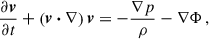
Equation (9) constitutes a quadratic eigenvalue problem (QEP). To solve this QEP, we linearise Eq. (9) to obtain the generalised eigenvalue problem Aa′=ωBa′, with newly defined matrices A, B, and eigenvectors a′. Further details on the solution method for this QEP are given in Appendix C. In addition, we applied other solution schemes for Eq. (9), including the linearised equations of Deheuvels et al. (2017) and the generalised DG92 formalism described in Appendix D. We find that the solution of the generalised eigenvalue problem and the alternative approaches yield nearly identical results in terms of the rotational splitting asymmetries (see Fig. E.1 for results obtained with the generalised DG92 formalism).
The eigenvectors of this eigenvalue problem provide the contribution coefficients, ai, to compute the near-degenerate eigenfunctions in Eq. (5). We note that NDEs are only expected to occur between modes that are close in frequency and are hence strongest among neighbouring frequencies. This is reflected in decreasing contribution coefficients ai, for increasing frequency differences and, in perturbation theory, this is expressed by the fact that expansions for these ai are in powers not just of δωij, but also of δωij/(ωi2 − ωj2). We confirm this by numerically solving the eigenvalue problem described by Eq. (9). The total contribution due to the interaction with other modes (i.e. the contribution of the off-diagonal elements) is highest for p-dominated modes. This is expected because of the smaller frequency differences between subsequent mixed modes.
4. Synthetic data
To explore the applicability of the linear inversion method discussed in Sect. 2, we tested it with different sets of synthetic data. Using the methods described in Sect. 3, we computed rotational splittings in the presence of NDEs.
To compute the synthetic data, we used an evolutionary track of a 1 M⊙ star with solar metallicity (Asplund et al. 2009), constructed with the Modules for Experiments in Stellar Astrophysics (MESA, r12778, Paxton et al. 2011, 2013, 2015, 2018, 2019; Jermyn et al. 2023, and references therein) stellar evolution code. We used the mesa equation of state and OPAL opacities (Iglesias & Rogers 1996) extended with low-temperature opacities from Ferguson et al. (2005). Convection was treated using the mixing-length theory (Böhm-Vitense 1958), with a mixing-length parameter αMLT = 1.8. In the following sections, we focus on a model from this evolutionary track, with a large frequency separation Δν ≈ 9 μHz and a frequency of maximum oscillation power νmax ≈ 100 μHz. We refer to this model as the ‘evolved model’. This model is identical to the ‘Δν = 9 μHz model’ in Ahlborn et al. (2025). We computed the large frequency separation, Δν, using the scaling relations of (Kjeldsen & Bedding 1995), with reference values from Themeßl et al. (2018), and the mass and radius of the stellar models. We computed oscillation frequencies and eigenfunctions using the stellar oscillation code GYRE (version 7.1, Townsend & Teitler 2013; Townsend et al. 2018). We generated the synthetic mode sets, including synthetic uncertainties, following Ahlborn et al. (2025). Each mode set contains 12 dipole modes across four radial orders centred around νmax. For each radial order, we selected the most p-dominated mode and two of the least g-dominated modes.
To compute the synthetic rotational splittings and the NDEs we assumed a synthetic rotation profile. We used a profile with a step at the base of the convective envelope and otherwise constant rotation rates, that is a two-zone model as defined by Klion & Quataert (2017), Ahlborn et al. (2020). In the following sections, we assume varying ratios of core to envelope rotation rates. We define the rotational splittings for m = ±1 as the differences of the frequencies obtained by solving the full QEP posed by Eq. (9) with different m, as described in Appendix C:
 (13a)
(13a)
 (13b)
(13b)
For comparison, symmetric rotational splittings, δωnℓm, symm, were computed using Eq. (1). The rotational splittings computed for m = ±1 are shown in the left panel of Fig. 1. For the chosen rotation rates, the differences between the splittings of different azimuthal orders are clearly visible. To illustrate the difference between the splittings of different m, we define the asymmetry of the splittings as
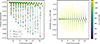 |
Fig. 1. Rotational splittings and their asymmetries as a function of mode frequency. Left panel: Rotational splittings of the evolved model using a core rotation rate Ωcore/(2π) = 750 nHz and an envelope rotation rate Ωenv/(2π) = 50 nHz. Rotational splittings that have the same npg are connected by a grey line. Only a subset of the rotational splittings centred around νmax ≈ 100 μHz is selected for the rotational inversions (see text for details). The dotted blue line connects the symmetric splittings for clarity. The rotational splittings, δωnℓm, were obtained by computing the frequency differences according to Eqs. (13a) and (13b), using the frequencies obtained from solving the full QEP posed by Eq. (9), as described in Appendix C, while the symmetric rotational splittings, δωnℓm, symm, where obtained from Eq. (1). Right panel: Asymmetries of the rotational splittings (Δωasym) of the evolved model over a range of core rotation rates Ωcore, for Ωenv/(2π) = 50 nHz. The lines are colour-coded by the core rotation rate. |
 (14)
(14)
This asymmetry is shown in the right panel of Fig. 1 for varying core rotation rates. The asymmetry increases with increasing core rotation rates. In the presence of a core magnetic field, the frequency perturbations would have the same sign for modes with different m. Therefore, the resulting asymmetries in the rotational splittings would not change sign as a function of frequency (see Li et al. 2022, their Fig. 2). Furthermore, magnetic frequency perturbations are expected to be higher for the g-dominated modes, as the magnetic field is typically assumed to be located in the core (e.g. Loi 2021; Bugnet et al. 2021). These features can be distinguished observationally from the pattern of asymmetries introduced by rotationally induced NDEs, as shown in the right panel of Fig. 1.
As input for the rotational inversions, we define ‘averaged’ dipole rotational splittings:
 (15)
(15)
because the linear inversions discussed in Sect. 2 assume a symmetric splitting following Eq. (1). A similar approach could be adopted for observed rotational splittings, particularly when no m = 0 component is visible. We invert this set of averaged rotational splittings using the rotational inversions and compare the estimated rotation rates to the known input rotation rates (see Sect. 5). The difference between the averaged splittings and the splittings for different m corresponds to half the asymmetry, Δωasym.
As an independent confirmation of the NDE formalism, we also computed the oscillation frequencies using a modified π–γ formalism (Ong & Basu 2020; Ong et al. 2021). The details are discussed in Appendix E. We find good agreement in the shape and magnitude of the asymmetries between both formalisms (see Fig. E.1). This agreement confirms the robustness of our synthetic data.
5. Impact of near-degeneracy effects
Near-degeneracy effects occur when the frequency difference between unperturbed modes is of the order of the rotational splittings, which scale with the star’s rotation rate; that is, |ω0, i − ω0, j|∼Ω (see DG92; Deheuvels et al. 2017; Li et al. 2024). Therefore, the error introduced by the NDEs in the linear inversion result is expected to depend on the star’s underlying rotation rate. The impact of NDEs is also expected to increase during evolution along the RGB (Deheuvels et al. 2017; Li et al. 2024). As stars evolve along the RGB, their cores contract while their envelopes expand. Overall, the mixed-mode density increases and the coupling strength decreases with evolution up the RGB, resulting in smaller frequency differences between mixed modes in each acoustic radial order and between p- and g-dominated mixed modes. Consequently, the impact of NDEs on rotational inversion results becomes more important in later evolutionary stages. This section first explores the dependence on the star’s position along the RGB, then discusses how the impact of NDEs varies with different rotation rates for a more evolved model with Δν ≈ 9 μHz. In the remainder of this section, we estimate the rotation rates of the core (Ωcore) and envelope (Ωenv) rotation rates by constructing averaging kernels at r0 = 0.003 and 0.98, respectively. To separate errors from NDEs from other sources (e.g. structural differences altering mixing fractions and rotational kernels, see Ong 2024) we inverted the synthetic rotational splittings using the stellar model from which the synthetic data were generated as a reference.
5.1. Lower RGB
To explore how NDE impacts vary along the lower RGB, we computed asymmetric rotational splittings along an evolutionary track using the forward model described in Sects. 3 and 4. We then inverted the core and envelope rotation rates using the averaged rotational splittings computed according to Eq. (15). Figure 2 shows that NDEs can be neglected for the least evolved stars, whereas for the most evolved stars, NDEs may lead to significant overestimation of envelope rotation rates and underestimation of core rotation rates.
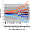 |
Fig. 2. Error in the estimated core and envelope rotation rates introduced by neglecting NDEs. The errors are shown in terms of the individual uncertainties, σΩ, as a function of the large frequency separation, Δν. Synthetic splittings were generated for three different core rotation rates, Ωcore/(2π) = 500, 750, and 1000 nHz, with an envelope rotation rate of Ωenv/(2π) = 50 nHz, indicated by crosses, circles, and squares, respectively. Results for the core and envelope are shown in shades of blue and red, respectively. Models evolve from left to right in this figure. |
In Fig. 2, models with high Δν resemble the star studied by Di Mauro et al. (2016, 2018), while models at the low end are closer to stars in the sample of Triana et al. (2017). Thus, the range of models in Fig. 2 covers the parameter space of red giants with currently available estimates of envelope rotation rates. We chose three representative core rotation rates (500, 750, and 1000 nHz) and one envelope rotation rate of 50 nHz1.
The deviation for the estimated envelope rotation rate is positive, while it is negative for the estimated core rotation rate along the evolution on the RGB – that is, the inversion procedure systematically overestimates envelope rotation rates and systematically underestimates core rotation rates. We note that observational uncertainties on the estimated envelope rotation rate range from approximately 12 nHz at the high end to 21 nHz at the low end of our Δν range, whereas the uncertainties of the estimated core rotation rates vary from 12 nHz to 16 nHz over the same range. Hence, a deviation of 2σ or larger very quickly becomes comparable to the underlying value of the envelope rotation rate and makes the result difficult to interpret. This is less problematic for the estimated core rotation rates, as the underlying values are typically ten times higher than those of the envelope rotation rates. The errors due to NDEs also become smaller with decreasing core rotation rate, as expected.
Based on these results, we identify ranges of core rotation rates and large frequency separations in which the linear inversions still provide accurate results for the given test case. For the case with a core rotation rate of 500 nHz or lower, NDEs do not appear to play a significant role along the evolution in the ranges considered here. For the intermediate case of 750 nHz, the estimated rotation rates become discrepant beyond 1σ for Δν ≈ 11 μHz. For the high core rotation rate of 1000 nHz, this occurs earlier, at Δν ≈ 13 μHz. Considering previous estimates of core rotation rates (Mosser et al. 2012; Triana et al. 2017; Gehan et al. 2018; Li et al. 2024), the transition from reliable estimates of the envelope rotation rate to unreliable estimates resides within the observed ranges of Δν and Ωcore. This highlights the importance of NDEs when interpreting linear rotational inversion results on the RGB.
5.2. Evolved model with Δν = 9 μHz
In this section, we explore the impact of NDEs on the inversion results for a single stellar model at the low Δν end in Fig. 2 in more detail (identical to the ‘Δν = 9 μHz model’ in Table 1 of Ahlborn et al. 2025, see also Sect. 4). We show the absolute error of the estimated envelope and core rotation rates for varying input core and envelope rotation rates in Fig. 3. These results demonstrate that core and envelope rotation rates can be recovered with small errors within certain limits of the underlying rotation rates, even for more evolved stars. This is equivalent to assuming that the rotational splittings can be approximated by Eq. (1) for sufficiently low rotation rates.
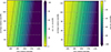 |
Fig. 3. Absolute error of the estimated envelope and core rotation rates for the evolved model. Left panel: Absolute error of the estimated envelope rotation rate as a function of the input core and envelope rotation rates. The input core and envelope rotation rates are given on the x- and y-axes, respectively. The error in the estimated envelope rotation rate, in units of nHz, is colour-coded and truncated at a maximum value of 100 nHz. Grey dots indicate the underlying grid of input core and envelope rotation rates. Contour lines are spaced by 10 nHz. Right panel: Same as in the left panel, but for the absolute error of the estimated core rotation rate. The colour scale is inverted because the errors on the core rotation rate are negative. |
The left panel of Fig. 3 reveals two immediate trends: (i) at fixed envelope rotation rate, the absolute error of the estimated envelope rotation rate increases with increasing core rotation rate, and (ii) for a fixed core rotation rate, the absolute error decreases with increasing envelope rotation rate. That is, the higher the ratio of the core-to-envelope rotation rates, the larger the error introduced in the estimated envelope rotation rate. However, the dependence of this absolute error on the input envelope rotation rate is much weaker than its dependence on the input core rotation rate: for an increase in the envelope rotation rate by a factor of five, the error decreases by approximately a factor of two to four, depending on the core rotation, whereas the error increases approximately by a factor of ten when the core rotation rate is doubled. This can be explained by the fact that the core rotates ten times faster than the envelope. A doubling of the core rotation rate therefore corresponds to a much larger absolute difference, indicating that the error in the estimated envelope rotation rate is dominated by the underlying core rotation rate.
As discussed above, the impact of the NDEs depends on the frequency differences between subsequent modes (i.e. modes with the same ℓ and m but different n) relative to the rotational splitting of the modes. In addition to the values of the core and envelope rotation rates, the rotational splitting depends on the shape of the underlying rotation profile. In most red giants, the g-modes are well described in the Jeffreys-Wentzel-Kramers-Brillouin (JWKB) regime, such that essentially all g-modes show the same sensitivity to the rotation rate. In the case of a rotation profile with a step at the base of the convection zone (used here), the entire g-mode cavity rotates at a constant rate. In a case with a more centrally concentrated rotation profile, for instance, one with a transition around the hydrogen-burning shell, the rotation rate changes within the g-mode cavity. This leads to smaller rotational splittings compared to the previous case because the g-mode component becomes sensitive to the more slowly rotating envelope (e.g. Ahlborn et al. 2022, 2025). However, from the perspective of NDEs, this is indistinguishable from the case where the core is set to rotate uniformly at an effective rotation rate averaged over the g-mode cavity. Thus, for the same reason that NDEs are less significant in slower-rotating cores, they are also less significant for more centrally concentrated rotational profiles.
The absolute errors for the estimated core rotation rates are shown in the right panel of Fig. 3. The trends are qualitatively the same as those for the estimated envelope rotation rate. Contrary to our findings for the envelope rotation rates, the core rotation rates are systematically underestimated when NDEs are neglected. Overall, the absolute errors in the core rotation rate are smaller than those in the envelope rotation rate. They do, however, remain of comparable magnitude. Considering that the core rotates about ten times faster than the envelope, the relative errors of the estimated core rotation rate are much smaller than those estimated for the envelope. From an analysis of Fig. 3 we conclude that, for the model under consideration, there is a range of core rotation rates within which we can neglect the effects of the NDEs and use linear rotational inversions. However, for high core rotation rates, this reinforces our earlier conclusion that envelope rotation rates are systematically overestimated, while core rotation rates are systematically underestimated.
6. Conclusions
We show that NDEs may have a significant impact on the rotational inversion results of red giant stars. This necessitates a careful interpretation of the core and envelope rotation rates estimated from techniques that inherently assume symmetric rotational splittings. However, we also show that, within certain limits of the internal rotation rates, linear rotational inversions remain applicable along the RGB. In this work, we used the eMOLA method, which typically delivers the most accurate envelope rotation rates. Considering the similarities with MOLA and SOLA inversions (e.g. Ahlborn et al. 2022, 2025), and in particular the use of Eq. (1), we conclude that our results provide a lower limit for the estimated envelope rotation rates.
Independent of the underlying rotation rates and position along the RGB, we find that the errors introduced in the estimated core and envelope rotation rates are of similar magnitude and have opposite signs (positive for the envelope, negative for the core). As the cores of red giants typically rotate ten to twenty times faster than their envelopes, the relative error on the estimated envelope rotation rate is much larger than on the core rotation rate. Relatively speaking, this makes estimated core rotation rates more reliable than the estimated envelope rotation rates: an error of 100 nHz on an estimated value of 1000 nHz still allows us to conclude that the core is rotating rapidly, whereas the same error on an estimate of 50 nHz renders reliable conclusions impossible. We therefore conclude that the estimated core rotation rates in the presence of NDEs can still be used to judge whether NDEs play a role.
We further demonstrate that the impact of NDEs varies strongly with evolution. As shown in Fig. 2, rotationally induced NDEs can be safely neglected for stars towards the base of the RGB, which is the case for the star analysed by Di Mauro et al. (2016). The NDEs arising from rotation alone are therefore not the dominant source of error in their linear rotational inversion results (see Ong (2024) for other sources). This remains true along the lower RGB for the lowest core rotation rate considered. For the higher core rotation rates of 750 and 1000 nHz, NDEs become significant (> 1σ) at Δν of approximately 11 μHz and 13 μHz, respectively. This implies that stars for which Triana et al. (2017) estimated high core rotation rates, most likely have estimated envelope rotation rates that are biased towards higher absolute values. Finally, we show that the error in the estimated rotation rates introduced by the NDEs increases strongly with increasing core rotation rate. This confirms earlier results by Deheuvels et al. (2017), Li et al. (2024).
The conclusions on the impact of NDEs are not exclusive to rotational inversions. Any method relying on Eq. (1) assumes a linear relation between rotational splitting and structural perturbation due to rotation. For example, RLS inversions employing Bayesian approaches (e.g. Beck et al. 2014; Fellay et al. 2021) relate rotational splittings, computed using a forward model, to either a frequency list or the power spectrum when evaluating likelihood functions. While the star analysed by Fellay et al. (2021) is still low on the RGB – where NDEs are not expected to play a role – the star studied by Beck et al. (2014) has evolved further up the RGB, where NDEs could introduce systematic errors. Such forward models therefore need to account for NDEs to obtain accurate estimates of the core and envelope rotation rates.
Despite the difficulties of estimating envelope rotation rates in the presence of high core rotation rates due to NDEs, we identify ranges in stellar parameters where the envelope rotation rates can still be recovered within the 1σ uncertainties. These ranges cover less evolved stars over a broader range of core rotation rates, as well as the lowest input core rotation rates for the more evolved model considered in Fig. 3. We expect that several Kepler red giants within the parameter ranges determined here can be analysed using linear inversion methods (e.g. eMOLA). This potential will be explored in future work.
These values cover the observed ranges of core and envelope rotation rates. In Sect. 5.2, we show that errors decrease with increasing envelope rotation rate, so results for larger envelope rotation rates are omitted here.
As the matrices L, R and D are real symmetric, the sets of left and right QEP eigenvectors coincide (e.g. Tisseur & Meerbergen 2001).
Acknowledgments
We would like to thank the anonymous referee for helpful comments to improve this manuscript. The research leading to the presented results has received funding from the European Research Council under the European Community’s Horizon 2020 Framework/ERC grant agreement no 101000296 (DipolarSounds). We thank the Klaus Tschira foundation for their support. JMJO acknowledges support from NASA through the NASA Hubble Fellowship grant HST-HF2-51517.001, awarded by STScI. STScI is operated by the Association of Universities for Research in Astronomy, Incorporated, under NASA contract NAS5-26555. SB acknowledges NSF grant AST-2205026. She would like to thank the Heidelberg Institute of Theoretical Studies for their hospitality at the time that this project was conceived. Throughout this work we have made use of the following Python packages: SCIPY (Virtanen et al. 2020), NUMPY (Harris et al. 2020), PANDAS (McKinney 2010), and MATPLOTLIB (Hunter 2007). We thank their authors for making these great software packages open source.
References
- Aerts, C., Christensen-Dalsgaard, J., & Kurtz, D. W. 2010, Asteroseismology (Dordrecht: Springer) [Google Scholar]
- Aerts, C., Mathis, S., & Rogers, T. M. 2019, ARA&A, 57, 35 [Google Scholar]
- Ahlborn, F., Bellinger, E. P., Hekker, S., Basu, S., & Angelou, G. C. 2020, A&A, 639, A98 [NASA ADS] [CrossRef] [EDP Sciences] [Google Scholar]
- Ahlborn, F., Bellinger, E. P., Hekker, S., Basu, S., & Mokrytska, D. 2022, A&A, 668, A98 [NASA ADS] [CrossRef] [EDP Sciences] [Google Scholar]
- Ahlborn, F., Bellinger, E. P., Hekker, S., Basu, S., & Mokrytska, D. 2025, A&A, 693, A274 [NASA ADS] [CrossRef] [EDP Sciences] [Google Scholar]
- Alvan, L., Mathis, S., & Decressin, T. 2013, A&A, 553, A86 [CrossRef] [EDP Sciences] [Google Scholar]
- Asplund, M., Grevesse, N., Sauval, A. J., & Scott, P. 2009, ARA&A, 47, 481 [NASA ADS] [CrossRef] [Google Scholar]
- Backus, G., & Gilbert, F. 1968, Geophys. J., 16, 169 [NASA ADS] [CrossRef] [Google Scholar]
- Beck, P. G., Hambleton, K., Vos, J., et al. 2014, A&A, 564, A36 [NASA ADS] [CrossRef] [EDP Sciences] [Google Scholar]
- Belkacem, K., Marques, J. P., Goupil, M. J., et al. 2015a, A&A, 579, A30 [NASA ADS] [CrossRef] [EDP Sciences] [Google Scholar]
- Belkacem, K., Marques, J. P., Goupil, M. J., et al. 2015b, A&A, 579, A31 [NASA ADS] [CrossRef] [EDP Sciences] [Google Scholar]
- Böhm-Vitense, E. 1958, Z. Astrophys., 46, 108 [Google Scholar]
- Bordadágua, B., Ahlborn, F., Coppée, Q., et al. 2025, A&A, 699, A310 [NASA ADS] [CrossRef] [EDP Sciences] [Google Scholar]
- Bugnet, L., Prat, V., Mathis, S., et al. 2021, A&A, 650, A53 [NASA ADS] [CrossRef] [EDP Sciences] [Google Scholar]
- Buldgen, G., Fellay, L., Bétrisey, J., et al. 2024, A&A, 689, A307 [NASA ADS] [CrossRef] [EDP Sciences] [Google Scholar]
- Cantiello, M., Mankovich, C., Bildsten, L., Christensen-Dalsgaard, J., & Paxton, B. 2014, ApJ, 788, 93 [Google Scholar]
- Ceillier, T., Eggenberger, P., García, R. A., & Mathis, S. 2013, A&A, 555, A54 [NASA ADS] [CrossRef] [EDP Sciences] [Google Scholar]
- Christensen-Dalsgaard, J., Schou, J., & Thompson, M. J. 1990, MNRAS, 242, 353 [NASA ADS] [Google Scholar]
- Deheuvels, S., García, R. A., Chaplin, W. J., et al. 2012, ApJ, 756, 19 [Google Scholar]
- Deheuvels, S., Ballot, J., Beck, P. G., et al. 2015, A&A, 580, A96 [NASA ADS] [CrossRef] [EDP Sciences] [Google Scholar]
- Deheuvels, S., Ouazzani, R. M., & Basu, S. 2017, A&A, 605, A75 [NASA ADS] [CrossRef] [EDP Sciences] [Google Scholar]
- Di Mauro, M. P., Ventura, R., Cardini, D., et al. 2016, ApJ, 817, 65 [NASA ADS] [CrossRef] [Google Scholar]
- Di Mauro, M. P., Ventura, R., Corsaro, E., & Lustosa De Moura, B. 2018, ApJ, 862, 9 [Google Scholar]
- Dyson, J., & Schutz, B. F. 1979, Proc. Royal Soc. London Ser. A, 368, 389 [Google Scholar]
- Dziembowski, W. A., & Goode, P. R. 1992, ApJ, 394, 670 [Google Scholar]
- Eggenberger, P., Miglio, A., Montalban, J., et al. 2010, A&A, 509, A72 [CrossRef] [EDP Sciences] [Google Scholar]
- Eggenberger, P., Montalbán, J., & Miglio, A. 2012, ApJ, 544, L4 [Google Scholar]
- Eggenberger, P., Lagarde, N., Miglio, A., et al. 2017, A&A, 599, A18 [CrossRef] [EDP Sciences] [Google Scholar]
- Eggenberger, P., den Hartogh, J. W., Buldgen, G., et al. 2019, A&A, 631, L6 [NASA ADS] [CrossRef] [EDP Sciences] [Google Scholar]
- Fellay, L., Buldgen, G., Eggenberger, P., et al. 2021, A&A, 654, A133 [NASA ADS] [CrossRef] [EDP Sciences] [Google Scholar]
- Ferguson, J. W., Alexander, D. R., Allard, F., et al. 2005, ApJ, 623, 585 [Google Scholar]
- Fuller, J., Lecoanet, D., Cantiello, M., & Brown, B. 2014, ApJ, 796, 17 [Google Scholar]
- Fuller, J., Piro, A. L., & Jermyn, A. S. 2019, MNRAS, 485, 3661 [NASA ADS] [Google Scholar]
- Gehan, C., Mosser, B., Michel, E., Samadi, R., & Kallinger, T. 2018, A&A, 616, A24 [NASA ADS] [CrossRef] [EDP Sciences] [Google Scholar]
- Goupil, M. J., Mosser, B., Marques, J. P., et al. 2013, A&A, 549, A75 [NASA ADS] [CrossRef] [EDP Sciences] [Google Scholar]
- Harris, C. R., Millman, K. J., van der Walt, S. J., et al. 2020, Nature, 585, 357 [NASA ADS] [CrossRef] [Google Scholar]
- Hunter, J. D. 2007, Comput. Sci. Eng., 9, 90 [NASA ADS] [CrossRef] [Google Scholar]
- Iglesias, C. A., & Rogers, F. J. 1996, ApJ, 464, 943 [NASA ADS] [CrossRef] [Google Scholar]
- Jermyn, A. S., Bauer, E. B., Schwab, J., et al. 2023, ApJS, 265, 15 [NASA ADS] [CrossRef] [Google Scholar]
- Käpylä, P. J. 2024, A&A, 683, A221 [NASA ADS] [CrossRef] [EDP Sciences] [Google Scholar]
- Kjeldsen, H., & Bedding, T. R. 1995, A&A, 293, 87 [NASA ADS] [Google Scholar]
- Klion, H., & Quataert, E. 2017, MNRAS, 464, L16 [NASA ADS] [CrossRef] [Google Scholar]
- Li, G., Deheuvels, S., Ballot, J., & Lignières, F. 2022, Nature, 610, 43 [NASA ADS] [CrossRef] [Google Scholar]
- Li, G., Deheuvels, S., & Ballot, J. 2024, A&A, 688, A184 [NASA ADS] [CrossRef] [EDP Sciences] [Google Scholar]
- Loi, S. T. 2021, MNRAS, 504, 3711 [NASA ADS] [CrossRef] [Google Scholar]
- Lynden-Bell, D., & Ostriker, J. P. 1967, MNRAS, 136, 293 [Google Scholar]
- Maeder, A. 2009, Physics, Formation and Evolution of Rotating Stars (Springer) [Google Scholar]
- Marques, J. P., Goupil, M. J., Lebreton, Y., et al. 2013, A&A, 549, A74 [NASA ADS] [CrossRef] [EDP Sciences] [Google Scholar]
- McKinney, W. 2010, in Proceedings of the 9th Python in Science Conference, eds. S. van der Walt, & J. Millman, 56 [Google Scholar]
- Mosser, B., Goupil, M. J., Belkacem, K., et al. 2012, A&A, 548, A10 [NASA ADS] [CrossRef] [EDP Sciences] [Google Scholar]
- Ong, J. M. J. 2024, ApJ, 960, 2 [NASA ADS] [CrossRef] [Google Scholar]
- Ong, J. M. J., & Basu, S. 2020, ApJ, 898, 127 [NASA ADS] [CrossRef] [Google Scholar]
- Ong, J. M. J., Basu, S., & Roxburgh, I. W. 2021, ApJ, 920, 8 [NASA ADS] [CrossRef] [Google Scholar]
- Ong, J. M. J., Bugnet, L., & Basu, S. 2022, ApJ, 940, 18 [NASA ADS] [CrossRef] [Google Scholar]
- Ouazzani, R. M., & Goupil, M. J. 2012, A&A, 542, A99 [NASA ADS] [CrossRef] [EDP Sciences] [Google Scholar]
- Paxton, B., Bildsten, L., Dotter, A., et al. 2011, ApJS, 192, 3 [Google Scholar]
- Paxton, B., Cantiello, M., Arras, P., et al. 2013, ApJS, 208, 4 [Google Scholar]
- Paxton, B., Marchant, P., Schwab, J., et al. 2015, ApJS, 220, 15 [Google Scholar]
- Paxton, B., Schwab, J., Bauer, E. B., et al. 2018, ApJS, 234, 34 [NASA ADS] [CrossRef] [Google Scholar]
- Paxton, B., Smolec, R., Schwab, J., et al. 2019, ApJS, 243, 10 [Google Scholar]
- Pijpers, F. P., & Thompson, M. J. 1992, A&A, 262, L33 [NASA ADS] [Google Scholar]
- Pijpers, F. P., & Thompson, M. J. 1994, A&A, 281, 231 [NASA ADS] [Google Scholar]
- Pinçon, C., Belkacem, K., Goupil, M. J., & Marques, J. P. 2017, A&A, 605, A31 [NASA ADS] [CrossRef] [EDP Sciences] [Google Scholar]
- Smeyers, P., & van Hoolst, T. 2010, in Linear Isentropic Oscillations of Stars: Theoretical Foundations (Berlin, Heidelberg: Springer), 371 [Google Scholar]
- Spada, F., Gellert, M., Arlt, R., & Deheuvels, S. 2016, A&A, 589, A23 [NASA ADS] [CrossRef] [EDP Sciences] [Google Scholar]
- Spruit, H. C. 2002, A&A, 381, 923 [CrossRef] [EDP Sciences] [Google Scholar]
- Suárez, J. C., Goupil, M. J., & Morel, P. 2006, A&A, 449, 673 [NASA ADS] [CrossRef] [EDP Sciences] [Google Scholar]
- Takahashi, K., & Langer, N. 2021, A&A, 646, A19 [NASA ADS] [CrossRef] [EDP Sciences] [Google Scholar]
- Themeßl, N., Hekker, S., Southworth, J., et al. 2018, MNRAS, 478, 4669 [Google Scholar]
- Tisseur, F., & Meerbergen, K. 2001, SIAM Rev., 43, 235 [Google Scholar]
- Townsend, R. H. D., & Teitler, S. A. 2013, MNRAS, 435, 3406 [Google Scholar]
- Townsend, R. H. D., Goldstein, J., & Zweibel, E. G. 2018, MNRAS, 475, 879 [Google Scholar]
- Triana, S. A., Corsaro, E., De Ridder, J., et al. 2017, A&A, 602, A62 [NASA ADS] [CrossRef] [EDP Sciences] [Google Scholar]
- Unno, W., Osaki, Y., Ando, H., Saio, H., & Shibahashi, H. 1989, Nonradial oscillations of stars (Tokyo: University of Tokyo Press) [Google Scholar]
- Virtanen, P., Gommers, R., Oliphant, T. E., et al. 2020, Nat. Methods, 17, 261 [Google Scholar]
Appendix A: Perturbed equation of motion
A generic equation of motion of a rotating fluid in the inertial frame is
 (A.1)
(A.1)
with v = Ω × r. By introducing Eulerian perturbations of the quantities in Eq. (A.1), one obtains that v0 = Ω × r and
 (A.2a)
 (A.2b)
if one assumes that  . It can be shown that
 (A.3a)
 (A.3b)
 (A.3c)
hold to first order in ξ for adiabatic oscillations, where Γ1 is the adiabatic index (∂lnp/∂lnρ)S (e.g. Smeyers & van Hoolst 2010). Substituting Eq. (A.3c) in Eq. (A.2b), one obtains
 (A.4)
(A.4)
where ℛv ≡ 2(v0⋅∇) and 𝒱v(ξ) ≡ (v0⋅∇)2ξ − (ξ⋅∇)(v0⋅∇)v0. Equation (A.4) is equal to Eq. (1.1) of Dyson & Schutz (1979) after multiplying by ρ0 and substituting the relations (A.2a), (A.3a) and (A.3b). Dropping the second-order term 𝒱v(ξ) in Eq. (A.4), and using the Ansatz ξ ∝ exp(−iωt), one recovers Eq. (6), because (see e.g. Aerts et al. 2010)
 (A.5)
(A.5)
Appendix B: Lowest-order perturbation theory
The frequency perturbation of mode i introduced by the rotational interaction with mode j can be computed from evaluating the generic matrix element ⟨ξ0, i | ℛξ0, j⟩ defined in Sect. 3:
 (B.1)
(B.1)
where the diagonal elements (i.e. δωii) signify the first-order frequency perturbations in the inertial frame (e.g. Eq. (19.48) of Unno et al. 1989, Eq. (3.261) and Eq. (3.265) of Aerts et al. 2010; see also DG92, Deheuvels et al. 2017, Sect. B.6.2 in Maeder 2009). Off-diagonal elements measure contributions from NDEs (DG92). We define the unnormalised displacement vector as
![Mathematical equation: $$ \begin{aligned} \boldsymbol{\tilde{\xi }} = \left[\tilde{\xi }_{\mathrm{r} } Y_\ell ^m\boldsymbol{e}_r+\tilde{\xi }_{\mathrm{h} }\left(\frac{\partial Y_\ell ^m}{\partial \theta }\boldsymbol{e}_\theta +\frac{1}{\sin \theta }\frac{\partial Y_\ell ^m}{\partial \phi }\boldsymbol{e}_\phi \right)\right]\mathrm{e}^{-{\mathrm{i} }\omega t}\,. \end{aligned} $$](/articles/aa/full_html/2025/12/aa55537-25/aa55537-25-eq32.gif) (B.2)
(B.2)
Here, Yℓm ≡ Yℓm(θ, ϕ) denote the spherical harmonics as defined in Aerts et al. (2010) with er, eθ and eϕ being the unit vectors of spherical polar coordinates and  denoting the unnormalised radial and horizontal displacement functions, respectively. Now we can compute the normalisation of the eigenfunction (Eq. (3.347) of Aerts et al. 2010):
![Mathematical equation: $$ \begin{aligned}&|\boldsymbol{\tilde{\xi }}_i|^2=\int _0^R\left[\tilde{\xi }_{{\mathrm{r} },i}^*\tilde{\xi }_{{\mathrm{r} },i}+\ell (\ell +1)\,\tilde{\xi }_{{\mathrm{h} },i}^*\tilde{\xi }_{{\mathrm{h} },i}\right]\rho _0(r)\,r^2\mathrm{d}r\,. \end{aligned} $$](/articles/aa/full_html/2025/12/aa55537-25/aa55537-25-eq34.gif) (B.3)
(B.3)
To compute the matrix element defined by Eq. (B.1), we normalise the radius-dependent parts of the displacement vector components –ξr and ξh– such that |ξ| = 1. For the sake of readability we drop the index 0 for the unperturbed modes in the remainder of this section. By evaluating the cross product originating from the Coriolis force (e.g. Eq. (3.342) of Aerts et al. 2010) we find
![Mathematical equation: $$ \begin{aligned}&\langle \boldsymbol{\xi }_i\,|\,({\mathrm{i} } m\Omega +\boldsymbol{\Omega }\times )\boldsymbol{\xi }_j\rangle \nonumber \\&= \int _V\rho _0(r)\,\boldsymbol{\xi }_i^*\cdot {\mathrm{i} } m\Omega (r)\,\boldsymbol{\xi }_j\,\mathrm{d}V + \int _V\rho _0(r)\,\boldsymbol{\xi }_i^*\cdot \boldsymbol{\Omega }\times \boldsymbol{\xi }_j\,\mathrm{d}V\,, \nonumber \\&= \,{\mathrm{i} } m \int _V\rho _0(r)\,\boldsymbol{\xi }_i^*\cdot \Omega (r)\,\boldsymbol{\xi }_j\mathrm{d}V \nonumber \\&+\int _V\rho _0(r)\,\boldsymbol{\xi }_i^*\cdot \nonumber \\&\left(\Omega (r)\left[-\xi _{{\mathrm{h} },j}\frac{\partial Y_\ell ^m}{\partial \phi }\boldsymbol{e}_r-\xi _{{\mathrm{h} },j}\frac{\cos \theta }{\sin \theta }\frac{\partial Y_\ell ^m}{\partial \phi }\boldsymbol{e}_\theta \right.\right.\nonumber \\&\left.\left.+\left(\xi _{{\mathrm{r} },j}\sin \theta Y_\ell ^m+\xi _{{\mathrm{h} },j}\cos \theta \frac{\partial Y_\ell ^m}{\partial \theta }\right)\boldsymbol{e}_\phi \right]\right)\,\mathrm{d}V\,. \end{aligned} $$](/articles/aa/full_html/2025/12/aa55537-25/aa55537-25-eq35.gif) (B.4)
(B.4)
This thus becomes:
![Mathematical equation: $$ \begin{aligned}&\langle \boldsymbol{\xi }_i\,|\,({\mathrm{i} } m\Omega +\boldsymbol{\Omega }\times )\boldsymbol{\xi }_j\rangle \nonumber \\&= \,{\mathrm{i} } m \int _V\rho _0(r)\,\boldsymbol{\xi }_i^*\cdot \Omega (r)\,\boldsymbol{\xi }_j\mathrm{d}V&\nonumber \\&+\int _V\rho _0(r)\,\Omega (r)&\nonumber \\&\left[\left(\xi _{{\mathrm{r} },i}Y_\ell ^m\right)^*\left(-\xi _{{\mathrm{h} },j}\frac{\partial Y_\ell ^m}{\partial \phi }\right)+\left(\xi _{{\mathrm{h} },i}\frac{\partial Y_\ell ^m}{\partial \theta }\right)^*\left(-\xi _{{\mathrm{h} },j}\frac{\cos \theta }{\sin \theta }\frac{\partial Y_\ell ^m}{\partial \phi }\right)\right.&\nonumber \\&\left.+\left(\xi _{{\mathrm{h} },i}\frac{1}{\sin \theta }\frac{\partial Y_\ell ^m}{\partial \phi }\right)^*\left(\xi _{{\mathrm{r} },j}\sin \theta Y_\ell ^m+\xi _{{\mathrm{h} },j}\cos \theta \frac{\partial Y_\ell ^m}{\partial \theta }\right)\right]\,\mathrm{d}V\,.&\end{aligned} $$](/articles/aa/full_html/2025/12/aa55537-25/aa55537-25-eq36.gif) (B.5)
(B.5)
In the second integral all terms contain the ϕ derivative of Yℓm, resulting in a multiplicative factor im for Yℓm. Note that the sign changes for some of the derivative terms due to complex conjugation. The integral in ϕ results in a multiplicative factor of 2π, as Yℓm and derivatives thereof always appear in pairs of complex conjugates. We can hence proceed to write:
![Mathematical equation: $$ \begin{aligned}&\langle \boldsymbol{\xi }_i\,|\,(im\Omega +\boldsymbol{\Omega }\times )\boldsymbol{\xi }_j\rangle \nonumber \\&= \,2\pi c_{\ell m}^2{\mathrm{i} } m\int _0^R\Omega (r)\,\rho _0(r)\int _0^\pi \nonumber \\&\left[\xi _{{\mathrm{r} },i}^*\xi _{{\mathrm{r} },j}\left(P_\ell ^m\right)^2+\xi _{{\mathrm{h} },i}^*\xi _{{\mathrm{h} },j}\left[\left(\frac{\partial P_\ell ^m}{\partial \theta }\right)^2+\frac{m^2}{\sin \theta }\left(P_\ell ^m\right)^2\right]\right]\,\sin \theta \mathrm{d}\theta \,r^2\mathrm{d}r\nonumber \\&+2\pi c_{\ell m}^2{\mathrm{i} } m\int _0^R\Omega (r)\,\rho _0(r)\int _0^\pi \nonumber \\&\left[-\left(\xi _{{\mathrm{r} },i}^*\xi _{{\mathrm{h} },j}+\xi _{{\mathrm{h} },i}^*\xi _{{\mathrm{h} },j}\right)\left(P_\ell ^m\right)^2-2\xi _{{\mathrm{h} },i}^*\xi _{{\mathrm{h} },j}\frac{\cos \theta }{\sin \theta }\frac{\partial P_\ell ^m}{\partial \theta }P_\ell ^m\right]\,\sin \theta \mathrm{d}\theta \,r^2\mathrm{d}r\,, \end{aligned} $$](/articles/aa/full_html/2025/12/aa55537-25/aa55537-25-eq37.gif) (B.6)
(B.6)
where we use
 (B.7)
(B.7)
Evaluating the integrals over the co-latitude θ, one finds:
![Mathematical equation: $$ \begin{aligned}&\langle \boldsymbol{\xi }_i\,|\,({\mathrm{i} } m\Omega +\boldsymbol{\Omega }\times )\boldsymbol{\xi }_j\rangle \nonumber \\ =&\,{\mathrm{i} } m\int _0^R\Omega (r)\,\rho _0(r)\nonumber \\&\left[\xi _{{\mathrm{r} },i}^*\xi _{{\mathrm{r} },j}+\ell (\ell +1)\,\xi _{{\mathrm{h} },i}^*\xi _{{\mathrm{h} },j}-\xi _{{\mathrm{h} },i}^*\xi _{{\mathrm{h} },j}-\left(\xi _{{\mathrm{r} },i}^*\xi _{{\mathrm{h} },j}+\xi _{{\mathrm{h} },i}^*\xi _{{\mathrm{r} },j}\right)\right]r^2\mathrm{d}r\,. \end{aligned} $$](/articles/aa/full_html/2025/12/aa55537-25/aa55537-25-eq39.gif) (B.8)
(B.8)
Together with Eq. (B.8) and the factor of −i from the operator (Eq. (B.1)) we can write down the expression for the perturbation due to rotation and define the kernel 𝒦ij:
![Mathematical equation: $$ \begin{aligned}&\delta \omega _{ij}=m\int _0^R\mathcal{K} _{ij}(r)\,\Omega (r)\mathrm{d}r\,,\nonumber \\&=m\int _0^R\Omega (r)\,\rho _0(r)\nonumber \\&\left[\xi _{{\mathrm{r} },i}^*\xi _{{\mathrm{r} },j}+\left(L^2-1\right)\xi _{{\mathrm{h} },i}^*\xi _{{\mathrm{h} },j}-\left(\xi _{{\mathrm{r} },i}^*\xi _{{\mathrm{h} },j}+\xi _{{\mathrm{h} },i}^*\xi _{{\mathrm{r} },j}\right)\right]r^2\mathrm{d}r\,, \end{aligned} $$](/articles/aa/full_html/2025/12/aa55537-25/aa55537-25-eq40.gif) (B.9)
(B.9)
(e.g. Deheuvels et al. 2017; Ong et al. 2022) with L2 = ℓ(ℓ + 1). Given the normalisation of the eigenfunctions ξi and ξj the total integral of the kernels 𝒦ij is written as
![Mathematical equation: $$ \begin{aligned} \beta _{ij}&=\frac{\int _0^R\left[\tilde{\xi }_{{\mathrm{r} },i}^*\tilde{\xi }_{{\mathrm{r} },j}+\left(L^2-1\right)\tilde{\xi }_{{\mathrm{h} },i}^*\tilde{\xi }_{{\mathrm{h} },j}-\left(\tilde{\xi }_{{\mathrm{r} },i}^*\tilde{\xi }_{{\mathrm{h} },j}+\tilde{\xi }_{{\mathrm{h} },i}^*\tilde{\xi }_{{\mathrm{r} },j}\right)\right]\rho _0(r)\,r^2\mathrm{d}r}{|\boldsymbol{\tilde{\xi }}_i||\boldsymbol{\tilde{\xi }}_j|}\,. \end{aligned} $$](/articles/aa/full_html/2025/12/aa55537-25/aa55537-25-eq41.gif) (B.10)
(B.10)
The ‘standard’ rotational kernel (see Eq. (1)) is obtained from that general expression for i = j:
![Mathematical equation: $$ \begin{aligned} \delta \omega _{ii}&=m\int _0^R\mathcal{K} _{ii}(r)\,\Omega (r)\mathrm{d}r\,,\nonumber \\&= \frac{m\int _0^R\left[\tilde{\xi }_{{\mathrm{r} },i}^2+\left(L^2-1\right)\tilde{\xi }_{{\mathrm{h} },i}^2-2\tilde{\xi }_{{\mathrm{r} },i}\tilde{\xi }_{{\mathrm{h} },i}\right]\rho _0(r)\,\Omega (r)\,r^2\mathrm{d}r}{\int _0^R\left[\tilde{\xi }_{{\mathrm{r} },i}^2+\ell (\ell +1)\,\tilde{\xi }_{{\mathrm{h} },i}^2\right]\rho _0(r)\,r^2\mathrm{d}r}\,, \end{aligned} $$](/articles/aa/full_html/2025/12/aa55537-25/aa55537-25-eq42.gif) (B.11)
(B.11)
assuming that the radial and horizontal displacement functions are real.
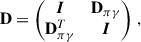
Appendix C: Solution of the NDE QEP
We solve the QEP of Eq. (9) by transforming it into a generalised linear eigenvalue problem of the form (this is the first companion form of Tisseur & Meerbergen 2001, with their N equal to – I):
 (C.1)
(C.1)
where we define new (right) eigenvectors2 a′ as
 (C.2)
(C.2)
The block matrices A and B are defined as
 (C.3a)
 (C.3b)
By definition, D = I (see Eq. (10c)) in this QEP. Hence, the generalised eigenvalue problem posed in Eq. (C.1) can be written as the augmented linear eigenvalue problem
 (C.4)
(C.4)
When solving the eigenvalue problem numerically using methods implemented in SCIPY, we find eigenvalues ω and −ω that are associated with the eigenfunction ξ defined by Eq. (5). The perturbed mode frequencies (when we include NDE) are then equal to the eigenvalues ω of Eq. (C.4), and the eigenvectors a can be extracted from the augmented eigenvectors a′.
Appendix D: Generalised NDE treatment of DG92
Instead of solving the QEP posed in Eq. (9) by linearising it into a generalised eigenvalue problem  , one can also generalise the treatment of NDE in Section 3.3 of DG92. We define the unperturbed frequency difference
 (D.1)
(D.1)
and the perturbed frequency as
 (D.2)
(D.2)
where ω0, i denotes the i-th unperturbed mode frequency of the near-degenerate modes and  is a perturbation to the frequency analogous to
  of DG92. If ω ≠ 0, we can equivalently write Eq. (9) as
 (D.3)
(D.3)
so that the elements on the diagonal of Z are
![Mathematical equation: $$ \begin{aligned} Z_{ii} = \Delta \omega _i -\omega _{0,i} - \tilde{\omega } + 2\delta \omega _{ii} + \dfrac{\omega _{0,i}}{\left(1 + \frac{[\tilde{\omega }-\Delta \omega _i]}{\omega _{0,i}}\right)}\,, \end{aligned} $$](/articles/aa/full_html/2025/12/aa55537-25/aa55537-25-eq54.gif) (D.4)
(D.4)
where we have used Eqs. (D.1) and (D.2). For nearly degenerate frequencies,  and Δωi are small compared to ω0, i, so that the diagonal elements of Z can be approximated by
 (D.5)
(D.5)
Denoting this approximation of Z as Z1, we can approximate the solution of the QEP posed in Eq. (9) by
![Mathematical equation: $$ \begin{aligned} \left[\dfrac{1}{2}\mathbf Z _1 + \text{ diag}\left(\tilde{\omega }\right)\right]\mathbf a \equiv \mathbf Z _2 \, \mathbf a = \tilde{\omega }\, \mathbf a \,. \end{aligned} $$](/articles/aa/full_html/2025/12/aa55537-25/aa55537-25-eq57.gif) (D.6)
(D.6)
Solving the eigenvalue problem Z2 a = 0 thus yields the perturbations  as eigenvalues, and a as eigenvectors.
Appendix E: Comparison to the π-γ decomposition
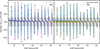 |
Fig. E.1. Comparison of rotational splitting asymmetries Δωasym computed from the NDE, generalised DG92 and π-γ formalisms. Results for the π-γ formalism and the generalised DG92 formalism are shown in the left and right panel, respectively. Here, the evolved model was used to compute the synthetic data. The shaded band indicates two times the minimum uncertainty of the averaged splittings obtained from Eq. (15). The multiplication by two is necessary because Δωasym is twice the frequency difference between the averaged and actual rotational splittings. As a minimum uncertainty of the observed frequencies we assume the frequency resolution. Then the minimum uncertainty of the averaged splittings is computed from error propagation as |

To validate the results that we obtained from the NDE formalism discussed in Sect. 3, we computed oscillation frequencies following the π-γ decomposition and recoupling described by Ong & Basu (2020), Ong et al. (2021). To include the effects of rotation we solve Eq. (9) in the π-γ basis. Here, the matrices are defined as follows:
 (E.1a)
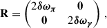 (E.1b)
 (E.1c)
where Ωπ2 = diag(ωπ, i2), Ωγ2 = diag(ωγ, i2) are diagonal matrices containing the unperturbed eigenfrequencies of the π and γ modes and δωπ = diag(δωπ, i) and δωγ = diag(δωγ, i) are diagonal matrices containing the rotational splittings of the π and γ modes computed according to Eq. (1). For the definitions of the other matrix elements Rππ, Rγγ, Rπγ, Dπγ we refer to Ong et al. (2021). We note that we have switched the sign in our definition of L in comparison to Ong et al. (2021) in order to comply with the definition of Eq. (9). We also take the time dependence of the oscillations (∝exp(−iωt)) into account. To solve the QEP posed by Eq. (9) and Eqs. (E.1a), (E.1b) and (E.1c) we transform it into a generalised Eigenvalue problem as in Eq. (C.1). In contrast to the NDE QEP defined in Appendix C we cannot rewrite the π-γ QEP into an augmented linear Eigenvalue problem.
Using the frequencies and eigenfunctions of the π- and γ-modes we computed the mixed mode frequencies for each azimuthal order m separately. Subsequently, we computed rotational splittings for each m, according to Eqs. (13a) and (13b) and the associated asymmetry Δωasym as the difference between the rotational splittings of different m according to Eq. (14). In Fig. E.1 we compare the asymmetries computed from the π-γ and NDE formalisms. We find good agreement both in terms of magnitude and find similar patterns of the asymmetries as a function of mode frequency. The formalisms compared here are independent methods to compute the rotational splittings. We consider this agreement an important validation of these methods.
All Figures
|
Fig. 1. Rotational splittings and their asymmetries as a function of mode frequency. Left panel: Rotational splittings of the evolved model using a core rotation rate Ωcore/(2π) = 750 nHz and an envelope rotation rate Ωenv/(2π) = 50 nHz. Rotational splittings that have the same npg are connected by a grey line. Only a subset of the rotational splittings centred around νmax ≈ 100 μHz is selected for the rotational inversions (see text for details). The dotted blue line connects the symmetric splittings for clarity. The rotational splittings, δωnℓm, were obtained by computing the frequency differences according to Eqs. (13a) and (13b), using the frequencies obtained from solving the full QEP posed by Eq. (9), as described in Appendix C, while the symmetric rotational splittings, δωnℓm, symm, where obtained from Eq. (1). Right panel: Asymmetries of the rotational splittings (Δωasym) of the evolved model over a range of core rotation rates Ωcore, for Ωenv/(2π) = 50 nHz. The lines are colour-coded by the core rotation rate. |
| In the text | |
|
Fig. 2. Error in the estimated core and envelope rotation rates introduced by neglecting NDEs. The errors are shown in terms of the individual uncertainties, σΩ, as a function of the large frequency separation, Δν. Synthetic splittings were generated for three different core rotation rates, Ωcore/(2π) = 500, 750, and 1000 nHz, with an envelope rotation rate of Ωenv/(2π) = 50 nHz, indicated by crosses, circles, and squares, respectively. Results for the core and envelope are shown in shades of blue and red, respectively. Models evolve from left to right in this figure. |
| In the text | |
|
Fig. 3. Absolute error of the estimated envelope and core rotation rates for the evolved model. Left panel: Absolute error of the estimated envelope rotation rate as a function of the input core and envelope rotation rates. The input core and envelope rotation rates are given on the x- and y-axes, respectively. The error in the estimated envelope rotation rate, in units of nHz, is colour-coded and truncated at a maximum value of 100 nHz. Grey dots indicate the underlying grid of input core and envelope rotation rates. Contour lines are spaced by 10 nHz. Right panel: Same as in the left panel, but for the absolute error of the estimated core rotation rate. The colour scale is inverted because the errors on the core rotation rate are negative. |
| In the text | |
|
Fig. E.1. Comparison of rotational splitting asymmetries Δωasym computed from the NDE, generalised DG92 and π-γ formalisms. Results for the π-γ formalism and the generalised DG92 formalism are shown in the left and right panel, respectively. Here, the evolved model was used to compute the synthetic data. The shaded band indicates two times the minimum uncertainty of the averaged splittings obtained from Eq. (15). The multiplication by two is necessary because Δωasym is twice the frequency difference between the averaged and actual rotational splittings. As a minimum uncertainty of the observed frequencies we assume the frequency resolution. Then the minimum uncertainty of the averaged splittings is computed from error propagation as |
| In the text | |
Current usage metrics show cumulative count of Article Views (full-text article views including HTML views, PDF and ePub downloads, according to the available data) and Abstracts Views on Vision4Press platform.
Data correspond to usage on the plateform after 2015. The current usage metrics is available 48-96 hours after online publication and is updated daily on week days.
Initial download of the metrics may take a while.