| Issue |
A&A
Volume 704, December 2025
|
|
|---|---|---|
| Article Number | A216 | |
| Number of page(s) | 9 | |
| Section | The Sun and the Heliosphere | |
| DOI | https://doi.org/10.1051/0004-6361/202556226 | |
| Published online | 12 December 2025 | |
Quantifying CME effects on plasma parameters and elemental abundance recovery during an M1 flare event with X-ray spectroscopy
1
Department of Physics, University of Helsinki, PO Box 64 00014 Helsinki, Finland
2
Isaware Oy, Dynamicum, Erik Palmenin Aukio 1, 00560 Helsinki, Finland
3
Leibniz-Institut für Astrophysik Potsdam (AIP), An der Sternwarte 16, D-14482 Potsdam, Germany
★ Corresponding author: This email address is being protected from spambots. You need JavaScript enabled to view it.
Received:
3
July
2025
Accepted:
19
October
2025
Aims. In this study, we examine the evolution of the plasma parameters, elemental abundances, and X-ray emission source during a long-duration M1-class solar flare and analyze the results in relation to the accompanying coronal mass ejection (CME).
Methods. We used SUNSTORM 1/XFM-CS soft X-ray data to study flare characteristics during an eruption that occurred on the Sun on June 24, 2024, from Active Region 13712. The XFM-CS data were fit with a two-component thermal model using PyXspec. Soft X-ray results were connected with X-ray image reconstructions from SolO/STIX data. The X-ray analysis was complemented with remote-sensing data from STEREO-A/SECCHI and EUVI, SOHO/LASCO, and SDO/AIA to provide a detailed account of the event.
Results. The CME onset corresponds to an increase in X-ray flux, plasma temperature, and emission measure. Prominent X-ray loops are observed in extreme ultraviolet (EUV) after the eruption and remain visible throughout the day. STIX imaging results reveal a large, gradually evolving thermal loop-top emission source. The first ionization potential (FIP) bias does not show signs of recovery even hours after the eruption for any of the fitted elements. The results strongly support the claim that the associated CME delays elemental abundance recovery, providing a connection between flares and CMEs that can be observed and studied with X-rays.
Key words: Sun: abundances / Sun: chromosphere / Sun: corona / Sun: coronal mass ejections (CMEs) / Sun: flares / Sun: X-rays / gamma rays
© The Authors 2025
 Open Access article, published by EDP Sciences, under the terms of the Creative Commons Attribution License (https://creativecommons.org/licenses/by/4.0), which permits unrestricted use, distribution, and reproduction in any medium, provided the original work is properly cited.
This article is published in open access under the Subscribe to Open model. This email address is being protected from spambots. You need JavaScript enabled to view it. to support open access publication.
1. Introduction
Solar eruptions are among the most magnificent manifestations of plasma phenomena observable on Earth. The key forms of eruptions include solar flares and coronal mass ejections (CMEs), the main drivers of space weather. Flares are observed as sudden releases of energy across the whole electromagnetic spectrum and are classified according to peak soft X-ray flux. Coronal mass ejections are large ejections of solar plasma and magnetic flux into the heliosphere that appear as large outward-moving plasma clouds in coronagraph images. The connection between flares and CMEs has been of interest for decades, and early studies have shown that a notable portion of CMEs are associated with flares (e.g., St. Cyr & Webb 1991; Harrison 1995). Various key relationships have already been identified, indicating that association rates depend on flare duration (Sheeley et al. 1983), flux, and fluence (Yashiro & Gopalswamy 2009). A latitudinal spatial relationship between flares and CMEs has been established (Yashiro et al. 2008), and flare class has been reported to correlate with CME mass (Aarnio et al. 2011). However, many details of this complex relationship remain unknown.
According to the standard flare model, also known as the CSHKP model (Carmichael 1964; Sturrock 1966; Hirayama 1974; Kopp & Pneuman 1976), a flare occurs when energy within a magnetic loop is released due to reconnection. Reconnection occurs in a vertical current sheet and causes both downward and upward particle acceleration. Downward-accelerated particles stream along magnetic field lines and hit the chromosphere. Chromospheric heating produces pressure gradients that form soft X-ray loops above the solar surface. Hard X-rays are observed at loop footpoints due to downward-streaming electrons, and above loop-tops near the reconnection site.
While some straightforward connections between flare X-ray properties and CME characteristics have been established, X-ray spectroscopy remains an underused method for probing the CME-flare relationship. X-ray spectroscopy can yield information about plasma temperature, emission measure, and elemental abundances in the flaring region. The temporal evolution of elemental abundances during solar flares has been studied extensively from soft X-ray observations (e.g., Nama et al. 2023; Mondal et al. 2021; Narendranath et al. 2020, 2014). These parameters are of particular interest because of the coronal first ionization potential (FIP) bias: the abundances of elements with low FIP, such as Mg, Al, and Fe, are elevated in the corona and chromosphere in comparison to the photosphere. Conversely, high FIP elements exhibit the inverse behavior, known as the inverse FIP bias, with larger abundances in the photosphere than in the corona (Laming 2015). During solar flares, the abundances of low FIP elements decrease toward photospheric values in the impulsive phase of the flare before recovery. This phenomenon is currently understood through the ponderomotive force model (Laming 2004). Reflection of magnetohydrodynamic waves at the upper chromosphere results in FIP fractionation, and a thin fractionation layer forms. During a flare, less fractionated photospheric material flows rapidly into the flaring loop, and photospheric abundances are observed for low FIP elements. Eventually, increased pressure slows down the inflow of plasma, and the loop begins to cool. As the plasma cools, its pressure decreases and is no longer capable of supporting the dense plasma within the loop, resulting in depletion (Fletcher et al. 2011). Loop depletion initiates flare decay, during which abundances recover to pre-flare levels (Widing & Feldman 2001; Laming 2017).
Recovery times have been found to depend on the time the plasma is trapped within the magnetic field (Woo et al. 2004; Feldman & Widing 2003). Although the evolution of the FIP bias during flares is well-established from previous studies, the effects of associated CMEs have not been investigated until recently. Lehtolainen et al. (2024) studied the evolution of elemental abundances of M- to X-class flares with and without CMEs, using spectral data from SUNSTORM 1/XFM-CS. Coronal mass ejection association was found to delay the recovery of elemental abundances, likely due to continued plasma flow after CME offset along open field lines connected to the CME core.
SUNSTORM 1 was a two-unit CubeSat, which operated between August 2021 and September 2024, at Sun-synchronous low-Earth orbit. Its sole payload was the X-ray Flux Monitor for CubeSats (XFM-CS; Lehtolainen et al. 2022), a non-imaging soft X-ray spectrometer capable of measuring soft X-ray emission from the Sun with energy resolution between 160 eV (beginning of life) and 180 eV (end of life) at 5.9 keV in a wide dynamic range that covers solar X-ray emission from A to X10 level. Due to its wide dynamic range, XFM-CS is well-suited especially for studying stronger M- and X-class solar flares, where the intensity of the X-ray emission varies by several orders of magnitude during flare evolution.
The evolution of an X-ray emission source can be investigated with X-ray image reconstructions. Generally, an X-ray image is obtained by reconstructing count data and/or visibilities. The Spectrometer/Telescope for Imaging X-rays (STIX; Krucker et al. 2020) on board Solar Orbiter (SolO; Müller et al. 2020) observes hard X-ray bremsstrahlung emission in the 4–150 keV range. It uses a bi-grid Fourier-transform technique for imaging on angular scales from 7 to 180 arcsec with a 1 keV energy resolution (at 6 keV) to provide diagnostics of hot flare plasma. By projecting the produced STIX maps onto extreme ultraviolet (EUV) images of the Sun, one can study the location and morphology of an emission source over time.
The focus of this study is the solar eruption event on June 24, 2024, from Active Region (AR) 13721, where a CME was observed in association with a long-duration M1-class flare. This unique event was characterized by a very slow rise phase and left behind significantly large and long-lasting post-eruption loops, whose emission dominated the X-ray spectrum. We study the CME effects on soft X-ray signatures by providing a thorough analysis of the event, using X-ray spectroscopy and imaging, supported by other remote-sensing data. Spectral fitting results are presented for plasma parameters and elemental abundances. These results are connected to X-ray image reconstructions overlaid with EUV images.
This paper is organized as follows. Data and methods are detailed in Section 2. The results are presented in Section 3, followed by discussion in Section 4. Finally, a summary and conclusions are provided in Section 5.
2. Data and methods
2.1. Remote-sensing observations
To study CME signatures, we used remote-sensing and in situ observations from Solar Orbiter (Müller et al. 2020), Solar and Heliospheric Observatory (SOHO; Domingo et al. 1995), Solar TErrestrial RElations Observatory-A (STEREO-A; Kaiser et al. 2008), and Solar Dynamics Observatory (SDO; Pesnell et al. 2012). The CME source region was investigated with EUV images from the Extreme Ultraviolet Imager (EUVI; Wuelser et al. 2004) on board STEREO-A, the Atmospheric Imaging Assembly (AIA; Lemen et al. 2012) instrument on board SDO, and the SolO Full Sun Imager of the Extreme Ultraviolet Imager (FSI/EUI; Rochus et al. 2020). The evolution of the CME was studied with white light coronagraph images taken by the SOHO Large Angle and Spectrometric COronagraph (LASCO; Brueckner et al. 1995) C2 and C3 imagers, and the Sun Earth Connection Coronal and Heliospheric Investigation (SECCHI; Howard et al. 2008) COR2 coronagraph on board STEREO-A. We compared XFM-CS flux data with data from the Geostationary Operational Environmental Satellite-R series (GOES-R; Krimchansky et al. 2004; Goodman et al. 2019) GOES-16 and GOES-18 satellites, which observe X-ray flux with the X-ray Sensors (XRS; Woods et al. 2024) on the GOES-R Extreme ultraviolet and X-ray Irradiance Sensors (EXIS; Machol et al. 2020). Finally, we used flare and CME data from the Space Weather Database Of Notifications, Knowledge, Information (DONKI1), provided by the Moon to Mars (M2M) Space Weather Analysis Office and hosted by the Community Coordinated Modeling Center (CCMC) at NASA’s Goddard Space Flight Center (GSFC).
2.2. XFM-CS
The event was observed in soft X-rays by the X-ray Flux Monitor for CubeSats (Lehtolainen et al. 2022) on board ESA’s SUNSTORM 1 mission. The spacecraft was launched to low-Earth orbit in August 2021, and concluded its mission in September 2024, having observed hundreds of solar flares during its operation. Its first scientific results have been analyzed in Lehtolainen et al. (2022) and Lehtolainen et al. (2024). These studies have demonstrated the instrument’s capability to provide high-quality data to study the evolution of plasma parameters and elemental abundances during solar eruption events.
XFM-CS uses a Silicon Drift Detector (SDD) and digital pulse processing that allows the instrument to process over 300000 X-ray photons per second without excessive pulse pile-up while maintaining an energy resolution of < 180 eV at 5.9 keV at the end of life, which is quite close to the Fano limit of silicon. Thus, XFM-CS provides spectroscopic data of solar X-rays in a dynamic range covering the solar flare intensity range from A to X10 level, which is about an order of magnitude wider than the dynamic ranges of previous instruments with comparable energy resolutions. The time resolution is 1 s for the broadband flux data and 60 s for the high-resolution spectrum data. The energy range of XFM-CS is 1–30 keV. The broadband flux values are given in six channels, whose energy bounds correspond to the broadband solar X-ray flux channels of GOES. The high-resolution spectrum data are given in 512 evenly spaced energy channels.
The orbital period of SUNSTORM 1 is 90 minutes, of which the satellite spends 38 minutes in Earth’s shadow. This causes periodic gaps in the observed data. Raw solar X-ray data are calibrated through the science processing pipeline, which converts the raw spectra to physical units. In this process, a response matrix file (RMF) and an auxiliary response file (ARF) are produced. They characterize the detector’s spectral response and the effective area of the detector as a function of photon energy, respectively. The intensity scale of the chosen event was about 1 ⋅ 10−5 Wm−2.
Due to the sensitivity of solid state detectors to electrons, the electron background of the instrument is estimated by counting events with energies above the instrument’s energy range. This background is subtracted from the calibrated data.
2.3. Spectral fitting
The X-ray data were analyzed with the PyXspec interface within the general X-ray spectral fitting package XSPEC (Arnaud 1996). Spectrum data were fit with the (Variable) Astrophysical Plasma Emission Code (VAPEC; Smith et al. 2001) model, an APEC thermal plasma model with variable abundances. The abundances are given with respect to the photospheric abundances from Anders & Grevesse (1989). The APEC model assumes a local thermodynamic equilibrium and is thus better for modeling lower intensity events. We fit two model components with linked abundances to each spectrum. During each fitting round, the abundances were fit in fixed groups of two to four elements, while the temperature and emission measure components were kept free. The purpose of limiting the number of free parameters in this way was to minimize the possibility of the fit converging toward a nonphysical local minimum. This process was repeated until the convergence criterion was fulfilled, after which all parameters were opened for the final fit to ensure the model was not stuck to a local minimum, and to provide correct errors for each value.
Flaring plasma is known to be multi-thermal (e.g., McTiernan et al. 1999; Warren et al. 2013; Caspi et al. 2014): it has a differential emission measure (DEM), i.e., the emission measure is distributed over temperature. However, deriving a well-constrained DEM is difficult due to the large dynamic range of coronal temperatures. Self-consistent DEM temperatures and emission measures require simultaneously fitting EUV and soft X-ray fluxes (Ryan et al. 2014). Two distinct temperature components were found in DEM models in the impulsive phase for C-class flares by Mithun et al. (2022). These likely correspond to emission from directly heated plasma in the X-ray loop, and evaporated plasma from the chromospheric footpoints. Our two-temperature model is an approximation of the distribution, but its limits are well known compared to DEM models.
The X-ray spectrum was fit between 01:01:45 UTC and 08:07:05 UTC for each individual 60 s spectrum. The integration time was long enough to allow for a fixed energy range between 1 to 12 keV. Fitting was concluded based on convergence of the χ2 statistic, determined by a less than 1% deviation of three consecutive iterations. The systematic uncertainty of the data, normally used to reflect the uncertainties in the instrument calibration, was set to 2% to provide a statistically better fit. In our analysis this uncertainty covers both the possible uncertainties in instrument calibration and the uncertainties that arise from the limitations of our model with two thermal components at different temperatures in representing plasma that in reality is multi-thermal.
We did not subtract the background from the spectra due to its significant variability and high intensity relative to the investigated event, caused by multiple active regions present on the Sun as well as ongoing smaller-scale flaring activity. Additionally, the magnetic structure of this long-duration event, approximated as a single large loop, is comprised of a series of smaller flaring loops in a wide range of evolutionary stages with respect to temperature and composition. Given these factors, it was not possible to fully separate the background and flaring loop emission, and attempting to subtract the background in this case results in unphysical values for the fitted parameters. However, as demonstrated later, the results show that the long-duration flare clearly dominates the abundance variations.
A total of eight elements with varying FIPs were fit: Al, Ca, Mg, Ni, Fe, Si (low FIP), S (mid FIP), and Ar (high FIP). The Ni values obtained were uncharacteristically high at the beginning of the event. This is likely due to a low count rate at the Ni K-shell ionization energy at 7.8 keV. When fitting at these energies, contribution to the statistic was very small, and the model tried to fit Ni based on its L-shell free-bound emission at 1–2 keV, where the count rate is higher. The low-energy end of the spectrum is also affected by K-shell free-bound emission from Ne and O, which can overestimate Ni values. While Ni has been included in all spectral fits, we chose to omit the Ni fitting curve from the results presented here for clarity.
Figure 1 shows an example spectrum from the early decay phase of the flare event. The fitting parameters for this spectrum are presented in Table 1. The model plasma temperature parameter is defined as the temperature multiplied by the Boltzmann constant; the emission measure is converted from the APEC norm and expressed in inverse of cubic centimeters. The fit errors for each parameter represent the 1σ uncertainty, i.e., the square root of the diagonal elements of the covariance matrix. Data points with fewer than 1 ⋅ 10−4 counts s−1keV−1cm−2 have been excluded from the figure, as the number of events is small and they do not have a significant effect on the fitting result.
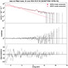 |
Fig. 1. Example solar X-ray spectrum of the early decay phase of the flare event at 05:51:50 UTC, observed by SUNSTORM 1/XFM-CS and fit for 1–12 keV using a two-component VAPEC model. Top panel: Data and folded model shown with hotter (dark red) and cooler (light red) model components. Middle panel: Data divided by the folded model. Bottom panel: Normalized fit residuals. |
Fitting results of an example spectrum during the event.
The cooler model component (light red) dominates at low energies (1–3 keV), while the hotter component (dark red) dominates at energies above 3 keV. The ratio shows a good fit at low energies but shows greater relative variation and increased noise above 6 keV. The statistical uncertainty is larger at higher energies due to the lower number of counts and the additional statistical fluctuations caused by the high-energy electron background (Lehtolainen et al. 2022). The bottom panel shows the fit residuals in terms of Poisson noise observed in the energy channels. Slightly greater variation is observed at low energies.
2.4. STIX
The temporal evolution of the emission source was investigated using data from the Spectrometer/Telescope for Imaging X-rays (Krucker et al. 2020) on board SolO. STIX is an imaging spectrometer that observes hard X-ray bremsstrahlung emission of flares in the 4 to 150 keV range. STIX uses a set of tungsten grids in front of 32 pixelated CdTe detectors to measure ten different angular resolutions on 7 to 180 arcsec scales (with three different orientations for each) with a 1 keV energy resolution (at 6 keV). STIX applies a discrete Fourier transform inversion to reconstruct the 2D brightness distribution of the X-ray emission. The STIX temporal resolution is dynamically adjusted: the data used in this study have a 12 s time resolution.
On June 24, 2024, SolO was positioned behind the western limb of the Sun at a distance of 0.95 AU with a Heliocentric Earth Equatorial (HEEQ) longitude of 166.62° and latitude of 3.74°. Absolute pointing information at the 4″ level cannot be provided at distances beyond 0.75 AU by the STIX Aspect System (SAS; Warmuth et al. 2020). This resulted in an 18″ offset in the y-direction for our event, determined by imaging the 04:52 flare peak in the 22 – 28 keV range where emission is mostly nonthermal. The contours were then aligned with the bright footpoint source observed in FSI/EUI 174 Å images. The offset is corrected in all maps presented in this study.
2.5. Image reconstruction
X-ray image reconstructions were made in the 6–10 keV range with an integration time of 60 s for the 02:30 to 08:00 interval to investigate the evolution of the emission source. To create the images, we used the 24 coarsest sub-collimators. To create the maps, we used the CLEAN imaging method (Högbom 1974; Schmahl et al. 2007), which produces a convolution of components with an idealized instrumental point spread function (PSF) by iterative deconvolution of the PSF from a dirty map created by the Back Projection algorithm (Massa et al. 2022). The 30%, 50%, and 70% intensity contours are shown projected onto 174 Å FSI/EUI images in Sect. 3.4.
3. Results
3.1. Event overview
AR 13712 was first observed on the surface of the Sun on June 12, 2024. By June 24, it had evolved into class βγ Eao and disappeared behind the western limb at S25W91. Several C- and M-class flares were observed when this active region moved across the solar disk, some of which were also associated with a CME. The CME eruption on June 24, 2024, from this source location, which is the main focus of this study, was observed by multiple instruments. The CME was associated with a long-duration flare event. A gradual increase in X-ray flux to the M1 level was observed from AR 13712, superposed with several impulsive events with no CME association. A comparison of GOES-16/XRS and GOES-18/XRS one-minute-averaged X-ray fluxes and SUNSTORM 1/XFM-CS flux in the GOES long (1–8 Å, 1.55–12.4 keV) and GOES short (0.5–4 Å, 3.1–24.8 keV) channels is shown in Figure 2, along with the SolO/STIX 6–10 keV light curve.
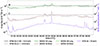 |
Fig. 2. X-ray flux observed in the GOES long (1.55–12 keV) and GOES short (3.1–24.8 keV) channels by SUNSTORM 1/XFM-CS (black, gray), GOES-16/XRS (dark green, dark mauve), and GOES-18/XRS (light green, light mauve). The SolO/STIX 6–10 keV light curve is shown in violet. The horizontal dashed lines mark the 10−5 and 10−6 GOES M- and C-class flux thresholds, respectively. Periodic data gaps are seen in XFM-CS data due to the instrument being in the Earth’s shadow. |
The fluxes show good agreement across all instruments: GOES-16 and GOES-18 fluxes are almost indistinguishable in the GOES long channel. It has been reported that fluxes observed by XFM-CS are generally 5–10% lower than the corresponding GOES long flux. GOES short flux matches very closely with XFM-CS during high flux and is usually higher than the corresponding XFM-CS flux during quiescent conditions (Lehtolainen et al. 2022). We observe a larger separation in the XFM-CS and GOES fluxes in the GOES short channel, with a closer match during the impulsive events. This is likely due to the different ways in which the variability of the shape of the X-ray spectrum is taken into account with the different instruments (Lehtolainen et al. 2022). The STIX light curve has a similar profile to the GOES and XFM-CS fluxes, with the highest counts observed during the impulsive flares.
An initial rise in X-ray flux is observed at 1:45 UTC, after which it begins to gradually rise around t ∼ 02 : 15. This marks the beginning of the long-duration event. Several impulsive flares occurred within the analyzed time period. According to the DONKI database, the peaks at 04:17 (associated with M1.3 flare), 04:52 (M1.8 flare), and 07:46 (M1.0 flare) also originate from AR 13712. During the decay of the long-duration flare, the X-ray flux first drops below the M level approximately at 05:30 UTC, followed by an increase due to a brightening starting at 06:59 UTC (M1.2 flare) from AR 13713. After this, the GOES long flux decays below the M level before another set of impulsive flares. The peak at 07:56 UTC is not cataloged but could be observed in EUV as a brightening near the loop footpoints at AR 13712.
Due to emission from other active regions, flux levels remained relatively high throughout the rest of the day. Flares from other active regions were not reported until 11:09 UTC. We limit our spectral analysis to the displayed time range, during which a gradual rise and decay can be identified, the main emission source is AR 13712, and sufficient time has passed after the eruption to reliably analyze its effects on the X-ray spectrum. It is noteworthy that no spectral radio signatures were associated with the long-duration event or the CME. This could be due to a lack of efficient electron acceleration as the event is extremely gradual.
The CME was observed in white light by the SOHO/LASCO C2 (1.5 to 6 solar radii) and C3 (3.7 to 30 solar radii), and STEREO-A/SECCHI COR2 (2 to 15 solar radii) coronagraphs (Figure 3). At the time of eruption, SOHO was located in the Earth-Sun L1 point at 1.01 AU at –0.1°, 2.1° (HEEQ longitude and latitude). STEREO-A was located at a distance of 0.95 AU from the Sun at 16.97°, 4.18° (HEEQ longitude and latitude). Due to the small spatial distance between the instruments, multipoint flux rope fitting of the CME in white light was not possible.
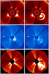 |
Fig. 3. Coronagraph observations of the CME by SOHO/LASCO C2 (top row) at 03:24 (left) and 04:28 (right), SOHO/LASCO C3 (middle row) at 06:42 (left) and 08:42 (right), and STEREO-A/SECCHI COR2 (bottom row) at 03:38:30 (left) and 06:53:30 (right). |
The CME first appeared in the SOHO/LASCO C2 field of view at 03:24 UTC, and a few minutes later at 03:38 UTC in STEREO-A/SECCHI COR2. We estimate the CME liftoff time to be close to 02:30 UTC based on the opening of field lines in SDO/AIA 193 Å images. A clear three-part CME structure can be seen in the white light images: a wide leading front, a dark cavity, and a bright core. The DONKI catalog reports a CME linear speed of 640 km/s, a direction of 91°, –40° (HEEQ longitude and latitude), and a half-width of 44°.
After the CME onset, prominent post-eruption loops formed above the solar surface. These structures appeared in STEREO-A/EUVI 304 Å images at 04:35:45 UTC and remained visible in EUV throughout the whole day. Figure 4 shows these loops at 06:45:45 UTC. The brightest part appeared at the loop-top, suggesting heating via magnetic reconnection. The hotter plasma can be observed from SDO/AIA 131 Å images, displayed in Figure 5. A supra-arcade fan (SAF) is visible above the flare arcades, and dark supra-arcade downflows (SADs) descending toward the loops are seen within the SAF over the hours after the eruption. This is an indicator of continuous reconnection in the current sheet extended behind the erupting flux rope (Bröse et al. 2022). It is evident from the brightness and longevity of the post-CME loops that they were a significant source of X-ray emission after the eruption.
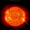 |
Fig. 4. STEREO-A/EUVI 304 Å image of the Sun on June 24, 2024, at 06:45:45 UTC. The bright post-CME loops indicated with the arrow are visible above the western limb, emerging from AR 13712 at S25W91. |
3.2. Plasma parameters
Fit results for temperature and emission measure are shown in Figure 6 along with the XFM-CS X-ray flux in the GOES long channel (black). The darker red and blue colors represent the plasma temperature (kT1) and emission measure (EM1) of the hotter component, while the lighter colors represent the temperature (kT2) and emission measure (EM2) of the cooler component.
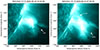 |
Fig. 5. SDO/AIA 131 Å images of the Sun on June 24, 2024, at 04:30:06 (left) and 07:00:06 (right) UTC. The arrows show the SAF, the post-CME loops, and the SADs. |
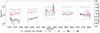 |
Fig. 6. Temporal evolution of emission measure and plasma temperature obtained with two-component VAPEC fitting, and SUNSTORM 1/XFM-CS X-ray flux (black). The temperature of the hotter component (dark red) peaks before the flux and corresponding emission measure (dark blue). The temperature (light red) and emission measure (light blue) of the cooler model component evolve steadily throughout the event. The emission measure axis is in logarithmic scale. |
Temperature and emission measure of both model components are observed to increase after CME onset. The hotter component shows more variability and has a stronger effect on the X-ray flux, while the cooler model component evolves relatively steadily throughout the event. EM1 increases by an order of magnitude after the eruption, and simultaneously the EM2 value doubles. While the long-duration event has a gradual profile, distinct temperature peaks preceding the peaks in emission measure are observed before the 04:17 and 04:52 UTC M-class flare peaks for the hotter component. Clear kT1 peaks are also seen for the 07:46 and 07:56 UTC impulsive events.
3.3. Elemental abundances
The fitting results for the evolution of elemental abundances are displayed in Figure 7. Elements are ordered by FIP energy: Al (FIP 6.0 keV, turquoise), Ca (FIP 6.1 keV, dark green), and Mg (FIP 7.6 keV, light green) are shown in the top panel; Fe (FIP 7.9 keV, dark purple) and Si (FIP 8.2 keV, light purple) are displayed in the middle panel; and the bottom panel displays the evolution of the mid-FIP element S (FIP 10.4 keV, dark pink) and the high-FIP element Ar (FIP 15.6 keV, light pink).
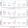 |
Fig. 7. Evolution of elemental abundances during the event for low-FIP elements Al, Ca, Mg (top panel), Fe, Si (middle panel), mid-FIP element S, and high-FIP element Ar (bottom panel). The horizontal dashed lines in each figure indicate photospheric abundances. |
A decrease in elemental abundances is clearly seen in the evolution of all low-FIP elements after CME onset. For low-FIP elements, abundances are 0.25 to 2.5 times higher before the eruption in comparison to the last fitted intervals. Al values decay significantly from 12 to 8, and Ca and Mg show a similar decay from 6 toward 3, with Mg abundances decaying slightly lower. Fe and Si abundances also show a clear decay toward photospheric levels after the eruption, from 3.0 to 1.5 and 2.5 to 1, respectively. For the mid-FIP element S we do not observe the expected inverse FIP bias. In contrast, it seems to behave as a low-FIP element, starting at 0.8 before the eruption and decaying toward 0.6 in the hours after. Ar values remain steady and close to photospheric during the event, with a slight increase expected for a high-FIP element after the CME liftoff.
The evolution of the reduced-fit statistic χ2 corresponding to the spectral fits displayed in Figures 6 and 7 is shown in Figure 8. The statistic varied between 1.5 and 3 during the fitting process, remaining close to 2 for most spectra. Slight peaks are seen around the strongest impulsive flares.
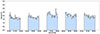 |
Fig. 8. Evolution of the reduced χ2 statistic during the fitting process. Larger values can be seen around the M-level flare peaks at 04:17 and 04:52. |
3.4. X-ray imaging
Imaging results obtained with the CLEAN reconstruction method detailed in Section 2.5 are presented in Figure 9 for the June 24, 2024, long-duration event. The 30%, 50%, and 70% contour levels are plotted over SolO FSI/EUI 174 Å images of the corona, showing the formation of the bright post-CME loops emerging from AR 13712 after the eruption.
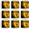 |
Fig. 9. STIX 30% (cyan), 50% (violet), and 70% (magenta) contours of the emission source in 6 – 10 keV obtained with the CLEAN imaging method, projected onto FSI/EUI 174 Å images of the Sun. The emission source expands and rises over time. |
A large loop-top source appears after the CME eruption. It is present in X-ray images already at 02:30:00–02:31:00 UTC, when the post-eruption loops are not yet visible in EUV. During the following hours, the source rises in the corona and increases in area. The gradual source remains visible throughout the full analyzed time period, except during the impulsive flares discussed in Section 3.1.
To further analyze the differences in morphology and location between the long-duration event associated with the CME and the impulsive flares linked to the same active region, we looked at STIX imaging results for the flare peaks at 04:17, 04:52, 07:46, and 07:56 UTC. For all impulsive events, STIX emission at 6 – 10 keV was observed near the loop footpoints. The sources were compact and short-lived in comparison to the gradual loop-top source. Although these events occur in the same active region as the long-duration event, their location and scale is distinctly different from the gradual source related to the CME.
4. Discussion
4.1. Soft X-ray spectroscopy
The evolution of temperature and emission measure can be understood through the standard flare model (Carmichael 1964; Sturrock 1966; Hirayama 1974; Kopp & Pneuman 1976). After CME onset, a steady increase in temperature and emission measure of both fitted components can be seen. Reconnection associated with the eruption leads to electron acceleration in the newly formed flare loops. The electrons stream along the magnetic field lines toward the footpoints, where they heat the chromosphere, and the heated plasma is conducted to the flare loop. Chromospheric evaporation is rapid, and the temperature peaks. Once the flaring loops are filled with chromospheric plasma, pressure increases, heating slows down, and emission measure peaks. Our fitting results for plasma parameters are consistent with the standard flare model. We also noticed that the hotter thermal component reacts more strongly to changes in X-ray flux. This component represents the high-temperature part of the DEM in our isothermal two-component parametrization of the temperature distribution and is enhanced due to the chromospheric evaporation of hot plasma during the flare process.
According to the ponderomotive force model, in the flare process, the FIP bias first depletes as unfractionated plasma fills the loops. Once the loops are filled, increased pressure impedes plasma flow (Fletcher et al. 2011), resulting in FIP bias recovery (Laming 2017). However, reestablishment of the FIP bias has been observed to take days in non-flaring active regions (Widing & Feldman 2001), suggesting that another process is required to explain the much faster FIP bias recovery observed during flares. An alternative explanation relies on flare-driven Alfvén waves that enhance the fractionation rate (Fletcher & Hudson 2008; Dahlburg et al. 2016), but such waves have not yet been observed (Mondal et al. 2021).
Our observations show a slow FIP bias depletion for low-FIP elements, which coincided with a gradual increase in X-ray flux and the launch of the associated CME. The FIP bias decreased most significantly right after the eruption for all elements except for the high-FIP element Ar, which increased. These variations were observed concurrently with increases in emission measure of both model components. In the last fitted intervals, the FIP bias decay slowed down, and significant changes in abundance were not seen for any of the fitted elements. Most notably, we did not observe a FIP bias recovery back toward pre-eruption levels within five hours after the eruption. This behavior can be attributed to the accompanying CME. If a flare is accompanied by a CME, some magnetic field lines remain connected to the CME core after the eruption. This decreases the pressure buildup within post-CME loops and allows the flow rate of matter through the fractionation layer to remain high for a longer time, which slows down FIP bias recovery (Lehtolainen et al. 2024).
Contrary to our expectations, the mid-FIP element S behaved similarly to a low-FIP element. This could be explained by chromospheric heating. If the temperature of the fractionation layer below the loop footpoints is sufficiently high to ionize the mid-FIP element, its abundance would be expected to behave as a low-FIP element within the loop. Closer investigation from remote sensing data was not possible due to the source location near the limb.
As discussed previously, we did not perform background subtraction due to the variability and relatively high intensity of background emission, which originates both from the flaring AR 13712 and from frequent smaller-scale activity elsewhere on the Sun. Consequently, reliable fitting with background subtraction was not possible in this case. Although the inclusion of background in our results may influence the observed variations, we also observe a clear increase in emission measure for both model components after the eruption. These pronounced changes strongly suggest that the simultaneously observed abundance variations are driven by the flare dynamics rather than the background.
4.2. Emission source
At low energies, X-ray emission is mostly thermal, and coronal loop-top sources are observed. Due to low density, such sources are not usually visible in EUV. Chromospheric footpoint sources are commonly observed at higher energies and appear bright in EUV, although sources have also been observed above the loop-top in more energetic flares (Masuda 1994; Masuda et al. 1995). Additionally, large coronal sources have been linked to long-duration soft X-ray events, while impulsive flares show strong emission from footpoint sources (Pallavicini et al. 1977).
Our X-ray imaging results show a large, gradually evolving coronal source associated with the CME, which expanded and rose over time. Compact footpoint X-ray sources were observed during all of the impulsive flares from AR 13712 that occurred during the long-duration event. These sources are clearly distinct from the loop-top X-ray source. Our results confirm that the gradual source was the dominant emission source in the 6–10 keV energy range during the analyzed time period.
5. Summary and conclusions
In this study, we investigated the long-duration solar eruption event of June 24, 2024, using SUNSTORM 1/XFM-CS spectra and SolO/STIX imaging data. Remote-sensing observations showed an extremely slow rise in X-ray flux followed by a CME from AR 13712. The CME left behind bright post-eruption loops, observed in EUV. The EUV images showed features indicating continuous current sheet reconnection. Imaging was performed in the 6–10 keV energy range, which revealed a large, expanding loop-top X-ray source associated with the eruption event.
Soft X-ray spectral fitting was done with two Maxwellian temperature components between 1–12 keV. Plasma parameter evolution followed the standard flare model, and the FIP bias was observed in time-series analysis of the elemental abundances. The recovery of abundances during the June 24, 2024, event was observed to be very slow. The abundances of the low-FIP elements Al, Ca, Mg, Fe, and Si decreased after the eruption and remained depleted for the analyzed time interval. S was observed to behave similarly to a low-FIP element, and a slight inverse FIP bias was seen for Ar. The observed prolonged decay of abundances is in agreement with the suggestion of (Lehtolainen et al. 2024) that the recovery of abundances is delayed after CME liftoff.
The established flare-CME connection observable with soft X-rays provides an interesting basis for more detailed studies of CME properties in relation to flare characteristics. Further statistical analysis is necessary to extract more information about the flare-CME relationship. Such knowledge could ultimately be used in space weather forecasting to characterize Earthward CMEs based on their accompanying flares. Furthermore, our results highlight the importance of considering associated CMEs in studies of elemental abundances during solar flares.
Acknowledgments
We thank the anonymous referee for their valuable comments that helped improve the manuscript. S.T. is funded by the Vilho, Yrjö and Kalle Väisälä Foundation. We acknowledge the Finnish Centre of Excellence in Research of Sustainable Space (Research Council of Finland grant numbers 352850 and 352846) and Research Council of Finland projects SolMer and FAISER (grant numbers 361480 and 361901). J.M. and A.W. are supported by the German Space Agency (DLR), grant number 50 OT 2304, as well as by the European Union’s Horizon Europe research and innovation program under grant agreement No. 101134999 (SOLER). Solar Orbiter is a space mission of international cooperation between ESA and NASA, operated by ESA. The STIX instrument is an international collaboration between Switzerland, Poland, France, Czech Republic, Germany, Austria, Ireland, and Italy. The EUI instrument was built by CSL, IAS, MPS, MSSL/UCL, PMOD/WRC, ROB, LCF/IO with funding from the Belgian Federal Science Policy Office (BELPSO); the Centre National d’Etudes Spatiales (CNES); the UK Space Agency (UKSA); the Bundesministerium für Wirtschaft und Energie (BMWi) through the Deutsches Zentrum für Luft- und Raumfahrt (DLR); and the Swiss Space Office (SSO). The SOHO/LASCO data used here are produced by a consortium of the Naval Research Laboratory (USA), Max-Planck-Institut fuer Aeronomie (Germany), Laboratoire d’Astronomie (France), and the University of Birmingham (UK). SOHO is a project of international cooperation between ESA and NASA. The STEREO/SECCHI and EUVI data used here are produced by an international consortium of the Naval Research Laboratory (USA), Lockheed Martin Solar and Astrophysics Laboratory (USA), NASA Goddard Space Flight Center (USA), Rutherford Appleton Laboratory (UK), University of Birmingham (UK), Max-Planck-Institut für Sonnensystemforschung (Germany), Centre Spatial de Liège (Belgium), Institut d’Optique Théorique et Appliqué (France), and Institut d’Astrophysique Spatiale (France). STEREO is a project of NASA. SDO/AIA data products are courtesy of NASA/SDO and the AIA, EVE, and HMI science teams. We acknowledge the Community Coordinated Modeling Center (CCMC) at Goddard Space Flight Center for the use of the The Space Weather Database Of Notifications, Knowledge, Information (DONKI), https://kauai.ccmc.gsfc.nasa .gov/DONKI/.
References
- Aarnio, A. N., Stassun, K. G., Hughes, W. J., & McGregor, S. L. 2011, Sol. Phys., 268, 195 [Google Scholar]
- Anders, E., & Grevesse, N. 1989, Geochim. Cosmochim. Acta, 53, 197 [Google Scholar]
- Arnaud, K. A. 1996, ASP Conf. Ser., 101, 17 [Google Scholar]
- Bröse, M., Warmuth, A., Sakao, T., & Su, Y. 2022, A&A, 663, A18 [NASA ADS] [CrossRef] [EDP Sciences] [Google Scholar]
- Brueckner, G. E., Howard, R. A., Koomen, M. J., et al. 1995, Sol. Phys., 162, 357 [NASA ADS] [CrossRef] [Google Scholar]
- Carmichael, H. 1964, NASA Spec. Publ., 50, 451 [NASA ADS] [Google Scholar]
- Caspi, A., McTiernan, J. M., & Warren, H. P. 2014, ApJ, 788, L31 [NASA ADS] [CrossRef] [Google Scholar]
- Dahlburg, R. B., Laming, J. M., Taylor, B. D., & Obenschain, K. 2016, ApJ, 831, 160 [CrossRef] [Google Scholar]
- Domingo, V., Fleck, B., & Poland, A. I. 1995, Sol. Phys., 162, 1 [Google Scholar]
- Feldman, U., & Widing, K. 2003, Space Sci. Rev., 107, 665 [CrossRef] [Google Scholar]
- Fletcher, L., & Hudson, H. S. 2008, ApJ, 675, 1645 [Google Scholar]
- Fletcher, L., Dennis, B. R., Hudson, H. S., et al. 2011, Space Sci. Rev., 159, 19 [Google Scholar]
- Goodman, S. J., Schmit, T. J., Daniels, J. M., & Redmon, R. J. 2019, The GOES-R Series: A New Generation of Geostationary Environmental Satellites (Elsevier) [Google Scholar]
- Harrison, R. A. 1995, A&A, 304, 585 [NASA ADS] [Google Scholar]
- Hirayama, T. 1974, Sol. Phys., 34, 323 [Google Scholar]
- Högbom, J. A. 1974, A&AS, 15, 417 [Google Scholar]
- Howard, R. A., Moses, J. D., Vourlidas, A., et al. 2008, Space Sci. Rev., 136, 67 [NASA ADS] [CrossRef] [Google Scholar]
- Kaiser, M. L., Kucera, T. A., Davila, J. M., et al. 2008, Space Sci. Rev., 136, 5 [Google Scholar]
- Kopp, R. A., & Pneuman, G. W. 1976, Sol. Phys., 50, 85 [Google Scholar]
- Krimchansky, A., Machi, D., Cauffman, S., & Davis, M. 2004, Proc. SPIE, 5570 [Google Scholar]
- Krucker, S., Hurford, G. J., Grimm, O., et al. 2020, A&A, 642, A15 [NASA ADS] [CrossRef] [EDP Sciences] [Google Scholar]
- Laming, J. M. 2004, ApJ, 614, 1063 [Google Scholar]
- Laming, J. M. 2015, Liv. Rev. Sol. Phys., 12, 4 [Google Scholar]
- Laming, J. M. 2017, ApJ, 844, 153 [Google Scholar]
- Lehtolainen, A., Huovelin, J., Korpela, S., et al. 2022, Nucl. Instrum. Meth. A, 1035, 23 [Google Scholar]
- Lehtolainen, A., Kilpua, E. K. J., & Huovelin, J. 2024, A&A, submitted [Google Scholar]
- Lemen, J. R., Title, A. M., Akin, D. J., et al. 2012, Sol. Phys., 275, 17 [Google Scholar]
- Machol, J. L., Eparvier, F. G., Viereck, R. A., et al. 2020, GOES-R Ser., 233 [Google Scholar]
- Massa, P., Battaglia, A. F., Volpara, A., et al. 2022, Sol. Phys., 297, 93 [NASA ADS] [CrossRef] [Google Scholar]
- Masuda, S. 1994, Ph.D. Thesis, Yohkoh HXT group, NAO, Mitaka, Tokyo [Google Scholar]
- Masuda, S., Kosugi, T., Hara, H., et al. 1995, PASJ, 47, 677 [NASA ADS] [Google Scholar]
- McTiernan, J. M., Fisher, G. H., & Li, P. 1999, ApJ, 514, 472 [CrossRef] [Google Scholar]
- Mithun, N. P. S., Vadawale, S. V., Zanna, G. D., et al. 2022, ApJ, 939, 112 [NASA ADS] [CrossRef] [Google Scholar]
- Mondal, B., Sarkar, A., Vadawale, S. V., et al. 2021, ApJ, 920, 4 [NASA ADS] [CrossRef] [Google Scholar]
- Müller, D., St. Cyr, O. C., Zouganelis, I., et al. 2020, A&A, 642, A1 [Google Scholar]
- Nama, L., Mondal, B., Narendranath, S., & Paul, K. T. 2023, Sol. Phys., 298, 55 [NASA ADS] [CrossRef] [Google Scholar]
- Narendranath, S., Sreekumar, P., Alha, L., et al. 2014, Sol. Phys., 289, 1585 [NASA ADS] [CrossRef] [Google Scholar]
- Narendranath, S., Sreekumar, P., Pillai, N. S., et al. 2020, Sol. Phys., 295, 175 [NASA ADS] [CrossRef] [Google Scholar]
- Pallavicini, R., Serio, S., & Vaiana, G. S. 1977, ApJ, 216, 108 [Google Scholar]
- Pesnell, W. D., Thompson, B. J., & Chamberlin, P. C. 2012, Sol. Phys., 275, 3 [Google Scholar]
- Rochus, P., Auchère, F., Berghmans, D., et al. 2020, A&A, 642, A8 [NASA ADS] [CrossRef] [EDP Sciences] [Google Scholar]
- Ryan, D. F., O’Flannagain, A. M., Aschwanden, M. J., & Gallagher, P. T. 2014, Sol. Phys., 289, 2547 [NASA ADS] [CrossRef] [Google Scholar]
- Schmahl, E. J., Pernak, R. L., Hurford, G. J., Lee, J., & Bong, S. 2007, Sol. Phys., 240, 241 [Google Scholar]
- Sheeley, N. R., Jr, Howard, R. A., Koomen, M. J., & Michels, D. J. 1983, ApJ, 272, 349 [NASA ADS] [CrossRef] [Google Scholar]
- Smith, R. K., Brickhouse, N. S., Liedahl, D. A., & Raymond, J. C. 2001, ApJ, 556, L91 [Google Scholar]
- St. Cyr, O. C., & Webb, D. F. 1991, Sol. Phys., 136, 379 [NASA ADS] [CrossRef] [Google Scholar]
- Sturrock, P. A. 1966, Nature, 211, 695 [Google Scholar]
- Warmuth, A., Önel, H., Mann, G., et al. 2020, Sol. Phys., 295, 90 [NASA ADS] [CrossRef] [Google Scholar]
- Warren, H. P., Mariska, J. T., & Doschek, G. A. 2013, ApJ, 770, 116 [Google Scholar]
- Widing, K. G., & Feldman, U. 2001, ApJ, 555, 426 [Google Scholar]
- Woo, R., Habbal, S. R., & Feldman, U. 2004, ApJ, 612, 1171 [Google Scholar]
- Woods, T. N., Eden, T., Eparvier, F. G., et al. 2024, J. Geophys. Res. Space Phys., 129, e2024JA032925 [Google Scholar]
- Wuelser, J.-P., Lemen, J. R., Tarbell, T. D., et al. 2004, SPIE Conf Ser., 5171, 111 [Google Scholar]
- Yashiro, S., & Gopalswamy, N. 2009, IAU Symp., 257, 233 [NASA ADS] [Google Scholar]
- Yashiro, S., Michalek, G., Akiyama, S., Gopalswamy, N., & Howard, R. A. 2008, ApJ, 673, 1174 [Google Scholar]
All Tables
All Figures
|
Fig. 1. Example solar X-ray spectrum of the early decay phase of the flare event at 05:51:50 UTC, observed by SUNSTORM 1/XFM-CS and fit for 1–12 keV using a two-component VAPEC model. Top panel: Data and folded model shown with hotter (dark red) and cooler (light red) model components. Middle panel: Data divided by the folded model. Bottom panel: Normalized fit residuals. |
| In the text | |
|
Fig. 2. X-ray flux observed in the GOES long (1.55–12 keV) and GOES short (3.1–24.8 keV) channels by SUNSTORM 1/XFM-CS (black, gray), GOES-16/XRS (dark green, dark mauve), and GOES-18/XRS (light green, light mauve). The SolO/STIX 6–10 keV light curve is shown in violet. The horizontal dashed lines mark the 10−5 and 10−6 GOES M- and C-class flux thresholds, respectively. Periodic data gaps are seen in XFM-CS data due to the instrument being in the Earth’s shadow. |
| In the text | |
|
Fig. 3. Coronagraph observations of the CME by SOHO/LASCO C2 (top row) at 03:24 (left) and 04:28 (right), SOHO/LASCO C3 (middle row) at 06:42 (left) and 08:42 (right), and STEREO-A/SECCHI COR2 (bottom row) at 03:38:30 (left) and 06:53:30 (right). |
| In the text | |
|
Fig. 4. STEREO-A/EUVI 304 Å image of the Sun on June 24, 2024, at 06:45:45 UTC. The bright post-CME loops indicated with the arrow are visible above the western limb, emerging from AR 13712 at S25W91. |
| In the text | |
|
Fig. 5. SDO/AIA 131 Å images of the Sun on June 24, 2024, at 04:30:06 (left) and 07:00:06 (right) UTC. The arrows show the SAF, the post-CME loops, and the SADs. |
| In the text | |
|
Fig. 6. Temporal evolution of emission measure and plasma temperature obtained with two-component VAPEC fitting, and SUNSTORM 1/XFM-CS X-ray flux (black). The temperature of the hotter component (dark red) peaks before the flux and corresponding emission measure (dark blue). The temperature (light red) and emission measure (light blue) of the cooler model component evolve steadily throughout the event. The emission measure axis is in logarithmic scale. |
| In the text | |
|
Fig. 7. Evolution of elemental abundances during the event for low-FIP elements Al, Ca, Mg (top panel), Fe, Si (middle panel), mid-FIP element S, and high-FIP element Ar (bottom panel). The horizontal dashed lines in each figure indicate photospheric abundances. |
| In the text | |
|
Fig. 8. Evolution of the reduced χ2 statistic during the fitting process. Larger values can be seen around the M-level flare peaks at 04:17 and 04:52. |
| In the text | |
|
Fig. 9. STIX 30% (cyan), 50% (violet), and 70% (magenta) contours of the emission source in 6 – 10 keV obtained with the CLEAN imaging method, projected onto FSI/EUI 174 Å images of the Sun. The emission source expands and rises over time. |
| In the text | |
Current usage metrics show cumulative count of Article Views (full-text article views including HTML views, PDF and ePub downloads, according to the available data) and Abstracts Views on Vision4Press platform.
Data correspond to usage on the plateform after 2015. The current usage metrics is available 48-96 hours after online publication and is updated daily on week days.
Initial download of the metrics may take a while.