| Issue |
A&A
Volume 704, December 2025
|
|
|---|---|---|
| Article Number | A108 | |
| Number of page(s) | 15 | |
| Section | Planets, planetary systems, and small bodies | |
| DOI | https://doi.org/10.1051/0004-6361/202556534 | |
| Published online | 09 December 2025 | |
Refractory element abundances in rocky planets and their host stars: Revisiting the compositional link
1
Institute of Science and Technology for Deep Space Exploration, Nanjing University,
Suzhou
215163,
PR China
2
State Key Laboratory of Lunar and Planetary Sciences, Macau University of Science and Technology,
Macau
999078,
PR China
★ Corresponding author: This email address is being protected from spambots. You need JavaScript enabled to view it.
Received:
22
July
2025
Accepted:
14
October
2025
Abstract
Context. Stars and planets form within the same protoplanetary disk, and hence their refractory element abundances are expected to share compositional links. Recent studies have revealed a pronounced non-1:1 relationship between the refractory element abundances of rocky exoplanets and their host stars. This finding is challenged by other works using updated stellar and planetary parameters.
Aims. We reanalyze the interior structure of rocky exoplanets by incorporating the updated observational constraints. Through a systematic assessment of model assumptions and statistical methods, we aim to resolve the existing discrepancies and advance our understanding of the compositional link between rocky exoplanets and their host stars.
Methods. We modeled the interior structure of 60 close-orbiting rocky exoplanets and derived their possible compositions using Bayesian statistical methods. Their bulk iron-to-silicate ratios were systematically compared with the refractory elemental abundances in their host stars, together with the core mass fraction as a first-order proxy for planetary bulk composition.
Results. Despite incorporating the updated measurements, we find that the planet-star compositional link maintains a non-1:1 relationship. It is demonstrated that both interior composition priors and uncertainty propagation methods significantly influence the derived planetary bulk compositions, thereby affecting the inferred star-planet compositional link. Moreover, a positive correlation between planetary iron content and stellar age is also identified, with younger stars hosting planets that are richer in iron. This is because the bulk compositions of rocky exoplanets show a clear correlation with the refractory abundances of their host stars, while the stellar chemical abundances serve as powerful proxies for ages.
Key words: planets and satellites: composition / planets and satellites: interiors / planets and satellites: terrestrial planets / stars: abundances
© The Authors 2025
 Open Access article, published by EDP Sciences, under the terms of the Creative Commons Attribution License (https://creativecommons.org/licenses/by/4.0), which permits unrestricted use, distribution, and reproduction in any medium, provided the original work is properly cited.
This article is published in open access under the Subscribe to Open model. This email address is being protected from spambots. You need JavaScript enabled to view it. to support open access publication.
1 Introduction
In the past few decades, an extensive array of exoplanets has been identified, encompassing categories such as hot Jupiters, sub-Neptunes, super-Mercuries, and super-Earths (Batalha 2014; Gillon et al. 2017). The Kepler survey identified over 2300 exoplanets throughout its nine-year mission, revealing high occurrence rates of close-in super-Earths and sub-Neptunes (Owen 2019), particularly prevalent around M stars (Dressing & Charbonneau 2013). The observed distribution of exoplanet radii reveals a radius valley located between super-Earths and subNeptunes, which has traditionally been attributed to the loss of a planet’s primordial hydrogen and helium (H/He) atmosphere. Recent studies suggest that the manifestation of the radius valley arises from the interplay of planetary formation (orbital migration) and evolutionary processes (atmospheric escape) (Burn et al. 2024). These exoplanets serve as vital subjects of scientific investigation, and examining their internal structures advances our understanding of planetary internal dynamics and formation processes (Kite & Barnett 2020).
Mass and radius constitute the primary observable characteristics of exoplanets, with the minimum mass being determined via radial velocity (RV) measurements, and the radius being ascertained through transit methods. Additionally, investigating the transmission and emission spectra of exoplanets provides valuable insights into their atmospheric composition. However, the observational data concerning atmospheric spectra are scant and primarily concentrated on hot Jupiters (Fairman et al. 2024; Smith et al. 2024). By comparing the observed mass and radius of a planet with the theoretical mass-radius curves, we can gain a first insight into its potential internal structure and composition (Seager et al. 2007; Zeng & Sasselov 2013). Nevertheless, inferring the internal structure of exoplanets using current massradius curves involves considerable uncertainties, as varying internal structures or compositions can account for the same set of observational data of mass and radius. In view of this, measurements of other observables have been discussed for small exoplanets to reduce the degeneracy. In particular, photospheric chemical abundances of host stars have been proposed as tracers to constrain the interior composition of small planets. Bayesian inference analysis has been extensively applied to constrain the internal structure and composition of exoplanets (Dorn et al. 2015, 2017; Liu & Ni 2023; Daspute et al. 2025). It combines the uncertainties of current measurements with the prior knowledge of variability in interior parameters, showing an advantage in exploring the ability of observable constraints. Dorn et al. (2015) demonstrated that integrating the abundance ratios of Fe/Si and Mg/Si derived from the host star, alongside the mass and radius measurements, substantially reduces the uncertainty in determining a planet’s internal structure when compared to methods relying solely on mass and radius data. In recent years, the rapid development of artificial intelligence, especially machine learning, has provided powerful tools for planetary science research and accelerated the understanding and exploration of planets. Machine-learning models have been used to study the internal structure of exoplanets and analyze the relationship between the overall characteristics of planets and their internal structure (Baumeister & Tosi 2023; Baumeister et al. 2020; Zhao & Ni 2021, 2022; Zhao et al. 2023). The performances of machinelearning and Bayesian inferences are also compared for the interior of rocky exoplanets with large compositional diversity (Zhao et al. 2024).
The advent of advanced spectrometers, such as MAROON-X, Keck Planet Finder (KPF), and HARPS-N, has facilitated the collection of a significant amount of high-precision RV data. This technological progress has allowed for the identification and more precise measurement of Earth-sized exoplanets in closein orbits. Due to the proximity of these Earth-sized planets to their host stars, both tidal (Jackson et al. 2009) and general relativity (Volpi & Libert 2024) effects considerably influence the long-term evolution of their orbits. Additionally, prevailing theories of planet formation suggest that these planets are unlikely to have formed in their current locations. Instead, they might have necessitated extensive material migration, or the planets may have originally formed in more distant orbits and subsequently migrated to their present positions (Schlichting 2014). Stars and planets formed at the same time and within the same protoplan-etary disk, suggesting that their refractory element abundance ratios are likely to be similar. This paradigm is strongly supported by our Solar System, where observational evidence and theoretical models demonstrate remarkable compositional consistency in refractory elements between the Sun, chondritic meteorites, and the terrestrial planets (Wanke & Dreibus 1994; Lodders 2003). Teske (2024) highlighted the connection between stellar compositions and exoplanet properties and reviewed the understanding of planet formation from stellar abundances. Plotnykov & Valencia (2020) and Schulze et al. (2021) analyzed the compositional characteristics of planets in relation to their host stars, concluding that rocky planets exhibit a broader spectrum of compositions relative to their host stars. Adibekyan et al. (2021) and Liu & Ni (2023) identified a pronounced non-1:1 relationship between the iron-mass fraction of planets and their host stars, including F, G, K stars and M dwarfs. Brinkman et al. (2024) and Brinkman et al. (2025) updated masses and radii for some rocky exoplanets and revisited the relationship between rocky exoplanets and stellar compositions, suggesting that rocky planets and their host stars exhibit the similar elemental abundance ratios. The compositional correlation between rocky exoplanets and host stars remains poorly constrained, limited by current uncertainties in observational data and variations in modeling methods.
In Sect. 2, we describe the sample with updated planetary and stellar measurements, the interior model of rocky exoplanets, the Bayesian inference of planetary compositions, and the determination of stellar parameters. In Sect. 3, we present the possible compositions of 60 close-orbiting rocky exoplanets. For a subset of 32 planets orbiting stars with measured elemental abundances, we analyze their bulk ratios of iron to major rock-building elements with respect to the stellar elemental abundances and system ages. The planet-star compositional relationships are quantified through rigorous statistical analysis. In Sect. 4, we interpret the observed discrepancies among the existing compositional relationships, explicitly accounting for variations in model assumptions and statistical treatments. We finally summarize the key aspects of our work in Sect. 5.
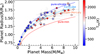 |
Fig. 1 Sample of selected exoplanets with radius measurements plotted as a function of mass and equilibrium temperature. Different colors denote the equilibrium temperature, Teq, of planets (zero albedo assumed). Dashed blue, light blue, and red lines, respectively, represent the M–R curves for pure-silicate, Earth-like, and pure-iron planets, derived by the interior model calculations. Critical masses of super Mercuries are labeled with dashed orange lines as a function of planetary radii, MSM = [0.25 + 0.87(R/R⊕)4.2]M⊕ (Unterborn et al. 2023). |
2 Methods
2.1 Sample selection
This study focuses on small exoplanets with masses under ten Earth masses (M⊕) and radii smaller than two Earth radii (R⊕), typically referred to as the transition zone between super-Earth and sub-Neptune. This is because the inherent degeneracy in interior structure and composition is considerably reduced without a significant volatile-rich envelope. Additionally, due to the large uncertainties in measurements of small-planets - especially in mass - we chose exoplanets in close-in orbits (orbital period <15 days). For small planets in close-in orbits, high-precision and high-cadence RV measurements were performed to enhance the precision in determining their masses and radii, with uncertainties in both measurements being less than 30%. This allows for more accurate constraints on planetary interiors. Finally, we selected 60 planets as the samples for our analysis, comprising 40 planets orbiting FGK stars and 20 planets orbiting M dwarfs. Fig. 1 presents the mass-radius distribution of our sample, with the theoretical mass-radius curves for four specific compositions: pure silicate, Earth-like, super-Mercuries, and pure iron. Within our sample, we identify two compositionally distinct populations based on their mass-radius positions: 21 planets are located around the M-R curve for pure silicon, suggesting that they could exhibit lower densities, and 13 planets are identified below the M-R curve for super-Mercuries, indicating their potential classification as super-Mercury candidates.
The 60 rocky exoplanets orbit 53 host stars, including 38 FGK-type and 15 M-dwarf systems. FGK stellar abundances have been well studied from high-resolution optical spectra (Brewer et al. 2016; Adibekyan et al. 2021; Brinkman et al. 2024, 2025). There are 32 FGK host stars that possess a complete set of elemental abundances for Fe, Mg, and Si. In contrast, measuring chemical abundances in M dwarfs is quite a difficult task due to their extremely blended spectral features, which complicate continuum placement and line measurements (Hejazi et al. 2024). Nevertheless, iron abundances [Fe/H] remain reliably measurable for M dwarfs. This is because iron has numerous weak lines in the near-infrared that are less blended compared to stronger transitions, and furthermore empirical calibrations for [Fe/H] are well established. Table A.1 summarizes the fundamental parameters for all 53 host stars in our sample. For several Kepler stars, recent spectroscopic measurements have achieved high precision, with typical abundance uncertainties of 0.01-0.02 dex (Liu et al. 2016, 2020). Nevertheless, to ensure internal consistency between stellar and planetary parameters, we prioritized using stellar abundances and planetary parameters derived from the same solution, for which stellar masses and radii used to compute planetary properties are consistent with those obtained from the stellar abundance analysis. In this work, we used such internally consistent data wherever available. In our sample of the 38 FGK stars, we find only ten systems for which the stellar abundances and planetary parameters originate from separate solutions: EPIC 249893012, HD 213885, K2-141, K2-216, Kepler-107, Kepler-105, Kepler-36, Kepler-99, KOI-1599, and TOI-431. Among the 15 M dwarfs, we identified only two systems: Kepler-138 and TRAPPIST-1. Previous spectroscopic comparisons have demonstrated that high-resolution spectra from different instruments frequently yield consistent stellar abundances. However, systematic differences persist among stellar abundance methods, even when applied to identical spectra (Hinkel et al. 2016). In our sample, the stellar relative chemical abundances for Fe, Mg, and Si are primarily sourced from Brinkman et al. (2024, 2025), Adibekyan et al. (2012b, 2021), and Brewer & Fischer (2018). The elemental ratio was calculated as [X/Y] = [X/H] - [Y/H], where the abundance [X/H] is defined as log (NX/NH)star — log (NX/NH)sun, using the solar photospheric abundances from Asplund et al. (2021). We compared the relative abundances for the host stars that these studies have in common in Figure 2. There are systematic method-dependent variations in [Fe/Mg] and [Si/Mg] among these three sources. For a robust statistical analysis, it is necessary to homogenize the abundance data from the different sources. We therefore adjusted the data from Adibekyan et al. (2012b, 2021) and Brewer & Fischer (2018), using the baseline established by Brinkman et al. (2024, 2025). The mean systematic deviations of Adibekyan et al. (2012b, 2021) and Brewer & Fischer (2018) from the Brinkman et al. (2024, 2025) baseline are −0.023 and 0.007 for [Fe/Mg], and −0.073 and 0.007 for [Si/Mg], respectively. We applied these mean deviations as zeropoint offsets to homogenize the stellar relative abundances from Adibekyan et al. (2012b, 2021) and Brewer & Fischer (2018).
2.2 Interior model of small planets
To explore the large compositional diversity of rocky exoplanets, the equilibrium mineralogy of the silicate mantle is best determined through the Gibbs free-energy minimization, as has been demonstrated by Dorn et al. (2015), Wang et al. (2019), and Unterborn et al. (2023). Dorn et al. (2015) provided a statistical inversion method to constrain the interior structures of rocky exoplanets from observational and model uncertainties, whereby the stellar elemental abundances are direct constraints on planetary bulk composition. Wang et al. (2019) employed a devolatilization model to predict detailed mantle compositions for individual planets, yielding geochemical insights that were deeper but applicable to a more limited sample (e.g., planets proximal to the habitable zone). The ExoPlex software package (Unterborn et al. 2023) provides discrete grids of mineralogical and thermoelastic parameters for a wide range of mantle compositions, thereby significantly enhancing the computational efficiency of the inversion process. In this work, we utilized the interior model ExoPlex to model the internal structure of small exoplanets. The model consists of three compositionally distinct layers: a water or ice outer shell, a silicate mantle, and an iron-rich core with small portions of light elements. Within the framework of the spherical approximation, the physical parameters within a planet are functions of the radius alone, such as density ρ(r), pressure P(r), and temperature T(r). The planetary interior adheres to the principles of hydrostatic equilibrium and mass conservation:
 (1)
(1)
 (2)
(2)
where m(r) is the mass within radius r, g(r) = −Gm (r)/r2 is the gravitational acceleration at radius r. The internal temperature is determined by the adiabatic temperature gradient,
 (3)
(3)
where α(P, T) and CP(P, T) represent the coefficients of thermal expansion and specific heat at constant pressure P, respectively. To solve the above equations, an equation of state (EOS) for the internal material is also required to describe the relationship between different thermodynamic state variables in a thermodynamic system:
 (4)
(4)
where the function, f, is contingent upon the composition of various shells. ExoPlex adopts the liquid iron EOS developed by Anderson & Ahrens (1994) for the iron-rich core, which is derived from shock compression experiments. For the mantle layer composed of silicates, ExoPlex utilizes the Perple_X thermodynamic equilibrium software (Connolly 2009) and adopts the underlying thermodynamic database of Stixrude & Lithgow-Bertelloni (2011) to determine ρi, CP,i, and αi. For the outermost layer of water or ice, ExoPlex employs the open-source Seafreeze software package (Journaux et al. 2020) to determine the different phases of H2O (liquid water, Ice Ih, II, III, V, or VI) and calculate the thermal expansion coefficients. The details regarding the interior model calculations can be found in Unterborn et al. (2023); Zhao et al. (2023).
Prior distributions of input parameters.
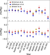 |
Fig. 2 Stellar elemental ratios [Fe/Mg] and [Si/Mg] from three data sources: Brinkman et al. (2024, 2025) (red), Adibekyan et al. (2012b, 2021) (blue), and Brewer & Fischer (2018) (yellow). |
2.3 Determination of planetary compositions
The ExoPlex forward calculation computes the radius (mass) of one planet by solving the coupled interior structure equations, given the total mass (radius) of the planet, water mass fraction (WMF), core mass fraction (CMF), and bulk molar ratios (Fe/Mg, Si/Mg, Al/Mg, Ca/Mg). In turn, the inverse problem solves for probable compositions from the observed mass and radius with measurement uncertainties. Here we used the affine invariant Markov chain Monte Carlo (MCMC) ensemble sampler emcee (Foreman-Mackey et al. 2013) to calculate the possible distribution of interior compositions. The emcee algorithm can explore the parameter space simultaneously through multiple “walkers” and efficiently handle complex posterior distributions. The prior distributions of each parameter are listed in Table 1. Considering that our selected planetary samples are situated close to their central stars, leading to a plausible assumption that these planets are devoid of water. Consequently, we first assigned the WMF at zero, thereby reducing the three-layer internal structure model to a two-layer configuration that includes solely a silicate mantle and an iron-rich core. For some planets with lower densities, we added a water or ice layer to stimulate the effect of volatile envelopes in Sect. 4.2. The prior distribution of total planetary masses was modeled as a Gaussian distribution with a mean of Mp and a standard deviation of σM, which were determined from the observed mass and corresponding uncertainty. The CMF is characterized by a uniform distribution ranging from 0.1 to 0.99, and the bulk molar Fe/Mg ratio follows a uniform distribution from 0 to 1.6. In contrast to Fe/Mg, which has the primary influence on the planetary radii, the bulk Si/Mg ratio has little influence on the planet radius. We adopted the stellar Si/Mg ratio as a prior for the planetary bulk Si/Mg, using a Gaussian distribution with a mean of Si/Mgstar and a standard deviation of σSi/Mg, where Si/Mgstar denotes the elemental abundance ratio Si/Mg of the host star, and σSi/Mg represents the associated measurement uncertainty. For cases in which stellar Si/Mg measurements are not available, we assumed their Si/Mg values follow a uniform distribution ranging from 0 to 1.6.
The likelihood function, p, was determined by the observed mass and radius and their uncertainties:
 (5)
(5)
A potential concern in the MCMC method is that of algorithmic convergence, particularly if the model parameters are estimated to be tightly correlated. Strong correlations can lead to inefficient sampling and high autocorrelation, leading to convergence problems. We assessed the convergence of each chain by estimating its autocorrelation time. In this work, the MCMC calculations generally converge within 5000 steps.
2.4 Determination of stellar parameters
For the host stars of exoplanets, our analysis focuses on two key stellar properties: refractory element abundances (Fe, Mg, Si) and stellar ages. The iron-mass fraction of host stars was inferred using the absolute stellar abundances (Adibekyan et al. 2021):
 (6)
(6)
where μX is the mean molecular weight of each species, X. Alternatively, the equivalent stellar CMF (CMFstar) was used to represent the iron mass to total iron and rock-building element mass (Brinkman et al. 2024). It was derived from the stellar Fe/Mg ratio by using the interior structure model SuperEarth (Plotnykov & Valencia 2020), assuming an Earth-like mantle composition (the mass ratio of Mg/Si ≈ 0.9). Similarly, we utilized the interior model ExoPlex to determine CMFstar from the Fe/Mg ratio of the host star, presuming that the remaining components are aligned with those of Earth, CMFstar:
 (7)
(7)
with  and
and  , where ωFeO is the mass fraction of FeO in the mantle.
Very recently Weeks et al. (2025) found that denser rocky planets are typically associated with younger stars. It is of interest to explore the correlation between rocky planet composition and stellar age. To determine the age of the host star, we employed the isochrones package (Morton 2015), a Pythonbased tool offering an accessible interface to various grids of stellar evolution models. Isochrones utilizes the emcee package to sample the joint posterior probability distribution of parameters such as age, mass, metallicity, distance, and extinction. In this work, we incorporated the effective temperature (Teff), surface gravity (log g), metallicity [Fe/H], Gaia magnitudes (G, BP, RP), and parallax (π̄) as input parameters. All these observations, with the exception of [Fe/H], were derived from Gaia DR3 (Gaia Collaboration 2016, 2023).
The main sequence stage of M dwarfs lasts for a long time, and most of their physical and observable properties do not change rapidly, making it difficult to infer their ages and requiring alternative methods such as gyrochronology (Engle & Guinan 2018; Angus et al. 2019) and kinematics (Almeida-Fernandes & Rocha-Pinto 2018). A more reliable age constraint can be obtained when one M dwarf is associated with a cluster or binary system where the companion has well-established isochronal or astereoseismic ages (Engle & Guinan 2018). Unlike the ages of the FGK stars derived through isochrone fitting, we adopted the published ages for the M dwarfs, which were determined through various methods. Crossfield et al. (2022) determined the age of GJ 1252 via gyrochronology using its rotation period. For the inactive thin-disk stars GJ 486 and TOI-1235, their ages were estimated empirically, resulting in larger uncertainties (Caballero et al. 2022; Bluhm et al. 2020). The age of Kepler-138 was derived using isochrone fitting (Morton et al. 2016). Bonfanti et al. (2024) derived the age of LTT 3780 through kinematic analysis incorporating Galactic space velocities (U, V, W) and Gaia DR3 reference coordinates. Finally, the age of TRAPPIST-1 was constrained through a combination analysis of lithium absorption, metallicity, kinematics, and rotational attributes (Burgasser & Mamajek 2017).
3 Results
Utilizing a two-layer interior model, we determined the internal structures of 60 rocky exoplanets by employing the MCMC method. As an example, Fig. B.1 presents the MCMC results of Kepler-10 b. The detailed results for the 60 exoplanets in our sample are summarized in Table A.2.
3.1 Relationship between the iron content of rocky planets and their host stars
We obtained the possible interior composition of rocky exoplanets, which enables us to explore the relationship between the elemental abundances of rocky planets and their host stars. The iron-mass fraction of a planet is given by
 (8)
(8)
where MFe,mantle and MFe,core denote the total mass of iron contained within the mantle and core, respectively. Fig. 3 shows the iron-mass fraction of the 60 rocky exoplanets as a function of the metallicity [Fe/H] of their host stars. One can see that a scarcity of planets were formed around the stars that have low iron content ([Fe/H] < -0.1), where most of these exoplanets possess the iron-mass fractions below 0.5. In the case of rocky exoplanets orbiting the host stars with the metallicity exceeding −0.1, there is an increase in the number of rocky planets, accompanied by a broader distribution range of the iron mass fraction. This is quite consistent with the conclusion of Liu & Ni (2023); Brinkman et al. (2024).
For purely rocky planets, the CMF is generally regarded as a first-order description of planetary bulk compositions. It is well known that iron distributes between mantle and core through planetary differentiation. When the iron-to-rock ratio in the mantle is known, the CMF has a one-to-one correspondence with the total iron-mass fraction, Feplanet%; otherwise, the CMF is dependent on the iron content of the mantle. Fig. 4 illustrates the resulting CMF of the 32 rocky exoplanets as a function of the equivalent stellar CMF. The planetary CMF and their uncertainties were computed from the MCMC calculations. The stellar CMFstar were calculated from the Fe/Mg ratio of the host stars using Eq. (7) with an Earth-like composition (Si/Mg=0.96, Al/Mg=0.09, Ca/Mg=0.07, and assuming no iron in the mantle, fFeO = 0). We also tested an Earth-like FeO content of fFeO = 8%, but this yielded only a minor reduction in all the CMFstar values, with a negligible impact on the overall conclusions of this work.
Our analysis reveals no statistically significant gap in CMF between super-Mercuries and super-Earths. This is consistent with the findings of Brinkman et al. (2025), and it is further quantified through the updated mass and radius measurements for some super-Mercuries (Brinkman et al. 2025). But some planets indeed have large CMF and Feplanet% values. The Fe/Mg ratio of Mercury within the Solar System markedly exceeds that found in both the Sun and Earth, with values ranging between 3.9 and 5.8 (Nittler et al. 2018). The prevailing perspective suggests that Mercury might have originally shared a similar Fe/Mg ratio with the Sun, subsequently gaining an elevated iron content due to substantial mantle-stripping collisions (Benz et al. 2007). These planets might have experienced substantial impacts similar to Mercury, or alternatively a series of smaller impacts, combined with processes such as the Mg-Fe-Si differentiation within the protoplanetary disk and the photo-induced evaporation. These mechanisms collectively contributed to their iron enrichment (Liu & Ni 2023). According to Unterborn et al. (2023), the threshold density for a super-Mercury is expressed as
![Mathematical equation: \rho_{\mathrm{SM}}=[4.6+1.5(R/R_{\oplus})^{2.1}] ~\mathrm{g\: cm}^{-3},](/articles/aa/full_html/2025/12/aa56534-25/aa56534-25-eq11.png) (9)
(9)
whereby a planet exceeding this density is likely to be categorized as a super-Mercury. Here we classify both Feplnet% > FeMercury% and ρ > pSM as super-Mercuries, and eight superMercuries are confirmed: Kepler-100b, Kepler-105c, Kepler-107c, HD 137496b, Kepler-406b, Kepler-99b, K2-229b, and GJ 367b. Apart from HD 137496b and GJ 367b, the host stars of the remaining six planets possess a complete set of elemental abundances for Fe, Mg, and Si. Additionally, we have identified several planets exhibiting lower densities, which are discussed in Sect. 4.2.
Two statistical methods were used to analyze the correlation between the CMF and CMFstar. First, we applied orthogonal distance regression (ODR, Boggs & Donaldson 1989) in the SciPy ODRPACK package to do linear regression to this sample. Unlike ordinary least squares (OLS) regression, which minimizes the vertical distances between the observed points and the fitted line, ODR minimizes the orthogonal distances, making it more suitable for cases where both variables have measurement errors. As is shown in Fig. 4, we conducted a linear fitting analysis, y = αx + β, on 26 super-Earth samples and found the correlation CMFplanet =(8.63 ± 2.71) × CMFstar − (2.28 ± 0.81), accompanied by a residual variance of 0.3527. For a direct comparison with Brinkman et al. (2024), we also employed their statistical methodology: using a Monte Carlo approach to sample the dataset of CMFstar and CMFplanet, followed by fitting these samples using OLS. After generating 10000 samples, we determined a slope of α =0.84 ± 0.76. Consistent with the findings of Brinkman et al. (2024), different linear regression approaches (e.g., ODR vs. OLS) yield statistically distinct slopes. Specifically, the slope difference in our analysis is even more pronounced than those reported by Brinkman et al. (2024). This enhanced sensitivity could be attributed to our extensive exploration of interior-model parameters that are capable of consistently accounting for the observational uncertainties. We provide a detailed discussion of these methodological considerations in Sect. 4.1.
We compared the iron-mass fractions of the 32 exoplanets with those of their host stars, as is shown in Fig. 5a. One can see that the iron-mass fractions in these planets are more enriched than in their host stars. The possible iron-enrichment mechanisms in rocky exoplanets are discussed in (Adibekyan et al. 2021; Liu & Ni 2023). Applying the ODR method to analyze super-Earth samples, we obtained the linear relationship Feplanet% =(14.03 ± 5.07) × Festar% — (4.12 ± 1.62) with a residual variance of 0.2172. From our analysis of the bulk molar ratios Fe/(Mg+Si) shown in Fig. 5b, we established the following correlation: Fe/(Mg + Si)planet =(18.88 ± 8.29) × Fe/(Mg + Si)star −(7.31 ± 3.46), with an associated residual variance of 0.1506. Combining the Monte Carlo approach with OLS regression, we also performed separate fits for both iron-mass fractions and bulk molar ratios Fe/(Mg+Si). The resulting slopes showed statistically significant differences from those obtained by ODR. As is demonstrated in Brinkman et al. (2025), the choice of statistical analysis methods (e.g., OLS vs. ODR) significantly influences the derived relationships between planetary and host-star chemical compositions. This discrepancy primarily arises from substantial uncertainties in both planetary interior compositions and stellar elemental abundances.
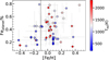 |
Fig. 3 Iron-mass fractions of the 60 rocky exoplanets versus metal-licities [Fe/H] of their host stars. The iron-mass fractions are inferred through the MCMC method combined with the two-layer interior model. |
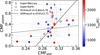 |
Fig. 4 Comparison of the CMF of the rocky exoplanets with the equivalent stellar CMFstar. The CMFstar values were calculated from the Fe/Mg ratio of the host stars using Eq. (7) with the Earth-like mantle composition [Si/Mg = 0.96, Al/Mg = 0.09, Ca/Mg = 0.07, and assuming no iron in the mantle, fFeo = 0 (Adibekyan et al. 2021; Brinkman et al. 2024)]. The rocky planets depicted by thin rhombuses are classified as super-Mercuries, while those illustrated with circles are identified as super-Earths. Solid and dashed black lines denote the ODR and OLS fits to the sample of the super-Earths, respectively. |
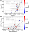 |
Fig. 5 Direct comparison of the iron-mass fractions (a) and the bulk molar ratios Fe/(Mg+Si) (b) of the 32 rocky exoplanets and their host stars. The compositions of the rocky exoplanets were inferred through the MCMC method combined with the two-layer interior model, whereas the compositions of the corresponding host stars were derived from the stellar elemental abundance ratios. |
3.2 Correlation between the iron content and stellar age of rocky planets
The ages of 38 FGK stars were determined through isochrone fitting. However, 12 of these exhibit large uncertainties, and furthermore the resulting stellar masses and radii have relatively large deviations from the literature values. To ensure the reliability of our age determinations, we excluded them from our analysis. The ages of this work were compared with those obtained by Weeks et al. (2025), as is shown in Fig. 6. The data points align well with the diagonal, showing good agreement between them. Combining these results with published M-dwarf ages, our final sample comprises 26 planets orbiting FGK stars and 11 orbiting M dwarfs. It is well known that the α elements (Mg, Si, S, and Ca), produced primarily via α-capture processes, serve as important chemical tracers. The [a/Fe] ratio constitutes a crucial indicator for distinguishing various stellar populations (Reddy et al. 2006). Notably, iron-poor planet-hosting stars frequently exhibit α-element enhancement (Adibekyan et al. 2012a). Fig. 7 shows the stellar [Mg/Fe] as a function of the stellar age. It seems that the host stars with higher [Mg/Fe] are predominantly older (Nissen 2015; Carrillo et al. 2023). For the old stars (>10 Gyr), the decreasing behavior of [Mg/Fe] with metallicities [Fe/H] is also evident (Recio-Blanco et al. 2014). Similar variations appear in the stellar [Si/Fe]-age relation. More specifically, Kepler-10 and TOI-561 show enhanced α-element abundances relative to iron, suggesting a population of thick disk stars (Dumusque et al. 2014; Weiss et al. 2021). In contrast, TOI-1444, K2-106, and HD 3167 have the near-solar metallicity [Fe/H] ≈ 0, requiring additional kinematic data to confirm their populations.
Since the stellar composition is correlated with its age, it is expected that the composition of rocky planets is linked to the age of their host stars. Fig. 8 illustrates the correlation between the iron-mass fraction of the 37 rocky exoplanets and the ages of their host stars. As before, we performed an ODR fit to the linear relation y = ax + β, resulting in a slope, a = −0.0455 ± 0.0095, and an intercept, β = 0.6871 ± 0.0799, with a residual variance of 1.8872. This negative correlation indicates an inverse relationship between the stellar age and the planetary iron-mass fraction, suggesting that younger stars tend to host iron-enriched planets. The host stars of all the known super-Mercuries have ages younger than 8 Gyr. Besides, the M-dwarf planets generally lie below the best-fit line, implying that there are distinct iron enrichment mechanisms for M dwarfs and FGK stars (Liu & Ni 2023).
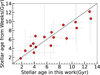 |
Fig. 6 Comparison of the stellar ages derived through isochrones in this work with those determined by Weeks et al. (2025). |
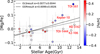 |
Fig. 7 Magnesium abundance [Mg/Fe] of the host stars as a function of the stellar age. Different colors indicate the metallicity, [Fe/H], of the host stars. |
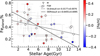 |
Fig. 8 Iron-mass fractions of the rocky exoplanets versus the ages of their host stars. The ages of FGK stars (denoted by circles) were determined through isochrones, while the ages of M dwarfs (denoted by inverted triangles) were derived from the previous works. |
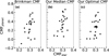 |
Fig. 9 Effects of the model assumptions and statistical methods: the CMF results of Brinkman et al. (2024, 2025) that were computed from the best literature values for planet mass and radius (a), the median of the CMF posterior distribution (b), and the optimal CMF that corresponds to the case in which the likelihood function reaches its minimum value in the MCMC chain (c). For the purpose of direct comparison, the planet samples selected here are consistent with Brinkman et al. (2024, 2025). |
4 Discussion
4.1 Different statistical methods
Despite analyzing the same planetary mass-radius data, our CMF estimates for rocky exoplanets differ from those of Brinkman et al. (2024, 2025). As is shown in Figures 9a and 9b, the CMF values reported by Brinkman et al. (2024, 2025) are generally lower than our median posterior estimates. In some cases there are even unphysical negative values (CMF < 0). We identify two primary sources for this discrepancy. First, Brinkman et al. (2024, 2025) fixed the mantle composition to the Earth-like values [olivine/pyroxene proportions of Xpy =0.6 and iron molar fractions of XFe =0.1] (Plotnykov & Valencia 2020) and assumed no silica inclusion in the iron core Xsi =0. That is, the bulk mass ratio Mg/Si was fixed at 0.9736 for all planets and the CMF had a one-to-one correspondence with the bulk ratio, Fe/Mg. In contrast, the CMF and mantle composition of our interior model were dynamically varied through the MCMC sampling: uniform priors for the CMF and bulk molar ratios Fe/Mg and Si/Mg, with the Si/Mg ratio initialized using Gaussian distributions centered on the host star’s Si/Mg ratio (when available). This allowed for a more robust exploration of the interior-model parameters, providing complete probability distributions for possible interior structures. For planets with small cores, these compositional differences significantly affect the CMF estimates, leading to the considerable differences in the CMF shown in Figures 9a and 9b. However, the effect becomes negligible for super-Mercuries, where core dominance minimizes the mantle contribution.
Second, Brinkman et al. (2024, 2025) applied conventional statistical techniques to first obtain a best-fit CMF through ξ2 minimization followed by uncertainty propagation, while our Bayesian approach directly samples the full joint posterior distribution of all model parameters via MCMC. With the fixed Earth-like mantle composition, the conventional methodology can yield unphysical negative CMF values when fitting certain planetary mass-radius observations. In contrast, our Bayesian framework with flexible mantle compositions maintains physical solutions across the entire parameter space. During the MCMC sampling, each step evaluates the likelihood function, P (Eq. (5)). We defined the optimal CMF as the solution with the highest statistical significance (i.e., the maximum P value). These optimal CMF values are plotted in Fig. 9c for direct comparison. We find excellent agreement between our optimal CMF values and those of Brinkman et al. (2024, 2025) for the coredominated planets (CMF > 0.4). However, for the planets with smaller cores (CMF < 0.4), the mantle composition, particularly its iron content, becomes the dominant factor influencing the CMF estimates.
To gain an insight into the variation in the mantle composition, we show the mantle molar ratios Fe/Mg and Si/Mg in Fig. 10, compared with the fixed mantle composition of Brinkman et al. (2024, 2025). The wide dispersion of the mantle ratios, relative to the fixed composition of Brinkman et al. (2024, 2025), provides a direct explanation for the differing CMF estimates between this work and Brinkman et al. (2024, 2025).
As is shown in Figure 4, the different linear regression approaches (ODR and OLS) yield statistically distinct slopes for the relationship between the CMF and CMFstar. This discrepancy could partially originate from the uncertainties in the stellar relative abundances. If the uncertainties in the stellar abundances for our sample were improved to the level achieved by Liu et al. (2016, 2020), in which the average uncertainty in [X/H] is approximately 0.025 dex, the resulting uncertainties in [Fe/Mg] and [Si/Mg] would be roughly 0.035 dex. The uncertainty in the recalculated CMFstar values ranges from approximately 0.018 to 0.026. Given this uncertainty, we reevaluated the relationship between CMF and CMFstar in Figure 11. The slopes derived from the two linear regression approaches show greater agreement compared to our previous results. Furthermore, if the average uncertainty in [X/H] was reduced to 0.01 dex, the slopes produced by the two approaches would become nearly identical. This indicates that advancements in the precision of stellar spectroscopy are essential for resolving the star-planet compositional relationship.
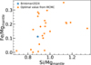 |
Fig. 10 Variations in the mantle compositions of Brinkman et al. (2024, 2025) and the present work. The mantle compositions are characterized by the molar ratios of Fe/Mgmantle and Si/Mgmantle. The fixed mantle composition from Brinkman et al. (2024, 2025) is denoted by blue pentagrams, whereas the mantle compositions from our optimal CMF samples are illustrated as orange circles. |
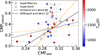 |
Fig. 11 Same as Figure 4, but with the equivalent stellar CMFstar values calculated using the reduced abundance uncertainty (σ[X/H] = 0.025 dex). For comparison, the ODR (solid orange) and OLS (dashed orange) fits from Figure 4 are also shown. |
4.2 Low-density exoplanets
Within our planetary sample, 17 targets displayed posterior mass-radius distributions that were statistically inconsistent with the observational measurements. Taking WASP-47 e as an illustrative example, we show the MCMC posterior probability distributions for its mass and radius in Fig. 12a. The primary reason for this deviation is the low density of these planets. Given an observed planetary mass, even extreme compositional adjustments (including CMF =0) fail to reconcile the resulting planetary radius with the observations. As is demonstrated in Fig. 1, all discrepant planets cluster near the pure silicate massradius curve, suggesting additional radius inflation mechanisms beyond our two-layer structure model.
All the selected planets occupy close-in orbits and likely formed with primordial H/He-dominated atmospheres. Over time, photo-evaporation typically strips away these volatiles, leaving behind bare rocky cores (Kite & Barnett 2020). However, planets with an initial high-molecular-weight atmosphere may develop more complex evolutionary pathways, potentially enabling the formation of secondary atmospheres (Kite & Barnett 2020). For a planet to accumulate and preserve a H/He-dominated atmosphere, it must possess a core of adequate size and maintain low temperatures (Ginzburg et al. 2016):
 (10)
(10)
where Mc is the mass of the core. According to this, it is improbable for these low-density planets to possess an atmosphere primarily composed of H/He. Instead, they are more likely to exhibit a volatile layer characterized by a higher average molecular weight. As is indicated by Brinkman et al. (2023), it is probable that TOI-561 b has a gaseous envelope consisting of species with a high mean molecular weight, such as water, carbon dioxide, or silicates. Meanwhile, Piette et al. (2023) proposed that HD 3167 b is a volatile-rich lava world, modeling its atmospheric temperature structure and thermal emission spectra for various volatile and rock-vapor compositions. Luo et al. (2024) suggest that most water on super-Earths can be sequestered in their interiors rather than on their surfaces, particularly for higher-mass planets. To account for exoplanets retaining substantial volatiles, we incorporated a water or ice layer, resulting in a three-layer structure consisting of an iron-rich core, a silicate mantle, and an outer water or ice envelope. Following the methodology described in Sect. 2.3, we employed MCMC sampling to constrain the posterior probability distributions of planetary interior compositions. The prior distribution of the WMF was taken as a uniform distribution ranging from 0 to 0.5, while the setting of the other parameters remained the same as in Sect. 2.3. The incorporation of the volatile layer results in an increased degeneracy of the internal components, necessitating approximately 20 000 steps for the MCMC calculation to achieve good convergence. As an example, Fig. B.2 presents the MCMC results for WASP-47 e. The detailed results of these 15 exoplanets are shown in Table A.3. Compared to the two-layer model, the three-layer model generally produces a higher iron-mass fraction and CMF. This discrepancy arises because the water or ice layer significantly increases the planet’s radius, requiring a larger core to offset its effect. Within our sample of the low-density planets, only five host stars possess high-precision abundance measurements, which is insufficient for statistically significant analysis. Furthermore, incorporating the results of the three-layer model produces negligible changes to our earlier findings.
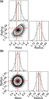 |
Fig. 12 MCMC posterior probability distributions for the mass and radius of WASP-47 e, derived from the two-layer model (a) and from the three-layer model (b). The median values, along with the ±1σ uncertainties, are depicted using dashed lines. The observed mass and radius are indicated by red lines. |
5 Conclusions
In this work, we combined the interior model ExoPlex with the MCMC method to constrain the possible interior compositions of the 60 rocky exoplanets in close-in orbits. The resulting planetary bulk compositions were statistically analyzed via a comparison with the stellar elemental abundance ratios and ages of their host stars. The planets formed around stars with higher metallicities exhibit a broader range in iron mass fractions. The rocky exoplanets generally demonstrate iron enrichment relative to their corresponding host stars. Furthermore, metal-poor stars with Mg enrichment tend to evolve at a slower pace. Combined with the established star-planet compositional correlation, this results in systematically lower iron mass fractions for the planets orbiting such older stars.
We have also discussed how the modeling assumptions and statistical approaches influence the inferred planet-star compositional relationships. The interior structures of rocky exoplanets remain degenerate due to limited observational constraints and large uncertainties in mass-radius measurements. Adopting any specific interior composition would artificially exclude viable solutions, potentially biasing inferences about planet-star compositional relationships. Given these challenges and current uncertainties in stellar abundances, a comprehensive statistical analysis should explore the complete parameter space of permissible interior structures and compositions that satisfy all observational constraints within their measurement uncertainties. Moreover, different treatments of measurement uncertainties and alternative statistical approaches could yield distinct planet-star compositional relationships. With improved measurements of both planetary parameters and stellar abundances, these effects would become less significant. Our analysis successfully resolves the apparent discrepancies between the planet-star compositional correlations reported by Adibekyan et al. (2021); Liu & Ni (2023) and those found in Brinkman et al. (2024, 2025).
For low-density planets, incorporating a volatile layer in interior structure modeling improves the interpretation of the observed mass and radius. However, this introduces substantial degeneracy in the inferred interior structure and composition. High-precision differential abundance analyses (Liu et al. 2016, 2020) for the host stars are essential to provide prior constraints on bulk planetary compositions. Further investigation of these low-density planets will require more precise measurements of planetary and stellar parameters and new observational constraints on planetary interiors such as atmospheric or surface characterization.
Acknowledgements
This work is supported by the National Natural Science Foundation of China (Grant No. T2495234, 12022517), the Pre-Research Projects on Civil Aerospace Technologies of China National Space Administration (Grant No. D010303), the Science and Technology Development Fund, Macau SAR (File No. 0139/2024/RIA2). This work has made use of data from the European Space Agency (ESA) mission Gaia (https://www.cosmos.esa.int/gaia), processed by the Gaia Data Processing and Analysis Consortium (DPAC, https://www.cosmos.esa.int/web/gaia/dpac/consortium). Funding for the DPAC has been provided by national institutions, in particular the institutions participating in the Gaia Multilateral Agreement.
References
- Adibekyan, V. Z., Delgado Mena, E., Sousa, S. G., et al. 2012a, A&A, 547, A36 [NASA ADS] [CrossRef] [EDP Sciences] [Google Scholar]
- Adibekyan, V. Z., Sousa, S. G., Santos, N. C., et al. 2012b, A&A, 545, A32 [NASA ADS] [CrossRef] [EDP Sciences] [Google Scholar]
- Adibekyan, V., Dorn, C., Sousa, S. G., et al. 2021, Science, 374, 330 [NASA ADS] [CrossRef] [Google Scholar]
- Agol, E., Dorn, C., Grimm, S. L., et al. 2021, PSJ, 2, 1 [NASA ADS] [Google Scholar]
- Almeida-Fernandes, F., & Rocha-Pinto, H. J. 2018, MNRAS, 476, 184 [Google Scholar]
- Almenara, J. M., Díaz, R. F., Dorn, C., Bonfils, X., & Udry, S. 2018, MNRAS, 478, 460 [CrossRef] [Google Scholar]
- Anderson, W. W., & Ahrens, T. J. 1994, J. Geophys. Res., 99, 4273 [NASA ADS] [CrossRef] [Google Scholar]
- Angus, R., Morton, T. D., Foreman-Mackey, D., et al. 2019, AJ, 158, 173 [Google Scholar]
- Asplund, M., Amarsi, A. M., & Grevesse, N. 2021, A&A, 653, A141 [NASA ADS] [CrossRef] [EDP Sciences] [Google Scholar]
- Azevedo Silva, T., Demangeon, O. D. S., Barros, S. C. C., et al. 2022, A&A, 657, A68 [NASA ADS] [CrossRef] [EDP Sciences] [Google Scholar]
- Batalha, N. M. 2014, Proc. Natl. Acad. Sci., 111, 12647 [NASA ADS] [CrossRef] [Google Scholar]
- Baumeister, P., & Tosi, N. 2023, A&A, 676, A106 [NASA ADS] [CrossRef] [EDP Sciences] [Google Scholar]
- Baumeister, P., Padovan, S., Tosi, N., et al. 2020, ApJ, 889, 42 [Google Scholar]
- Benz, W., Anic, A., Horner, J., & Whitby, J. A. 2007, Space Sci. Rev., 132, 189 [CrossRef] [Google Scholar]
- Bluhm, P., Luque, R., Espinoza, N., et al. 2020, A&A, 639, A132 [NASA ADS] [CrossRef] [EDP Sciences] [Google Scholar]
- Boggs, P. T., & Donaldson, J. R. 1989, Orthogonal Distance Regression (Hoboken: Wiley) [Google Scholar]
- Bonfanti, A., Brady, M., Wilson, T. G., et al. 2024, A&A, 682, A66 [NASA ADS] [CrossRef] [EDP Sciences] [Google Scholar]
- Bonomo, A. S., Zeng, L., Damasso, M., et al. 2019, Nat. Astron., 3, 416 [Google Scholar]
- Brewer, J. M., & Fischer, D. A. 2018, ApJS, 237, 38 [NASA ADS] [CrossRef] [Google Scholar]
- Brewer, J. M., Fischer, D. A., Valenti, J. A., & Piskunov, N. 2016, ApJS, 225, 32 [Google Scholar]
- Brinkman, C. L., Weiss, L. M., Dai, F., et al. 2023, AJ, 165, 88 [NASA ADS] [CrossRef] [Google Scholar]
- Brinkman, C. L., Polanski, A. S., Huber, D., et al. 2024, AJ, 168, 281 [Google Scholar]
- Brinkman, C. L., Weiss, L. M., Huber, D., et al. 2025, AJ, 170, 109 [Google Scholar]
- Burgasser, A. J., & Mamajek, E. E. 2017, ApJ, 845, 110 [Google Scholar]
- Burn, R., Mordasini, C., Mishra, L., et al. 2024, Nat. Astron., 8, 463 [Google Scholar]
- Caballero, J. A., González-Álvarez, E., Brady, M., et al. 2022, A&A, 665, A120 [NASA ADS] [CrossRef] [EDP Sciences] [Google Scholar]
- Cadieux, C., Plotnykov, M., Doyon, R., et al. 2024, ApJ, 960, L3 [NASA ADS] [CrossRef] [Google Scholar]
- Carrillo, A., Ness, M. K., Hawkins, K., et al. 2023, ApJ, 942, 35 [NASA ADS] [CrossRef] [Google Scholar]
- Connolly, J. A. D. 2009, Geochem. Geophys. Geosyst., 10, Q10014 [Google Scholar]
- Crossfield, I. J. M., Malik, M., Hill, M. L., et al. 2022, ApJ, 937, L17 [NASA ADS] [CrossRef] [Google Scholar]
- Dai, F., Masuda, K., Winn, J. N., & Zeng, L. 2019, ApJ, 883, 79 [NASA ADS] [CrossRef] [Google Scholar]
- Daspute, M., Wandel, A., Kopparapu, R. K., et al. 2025, ApJ, 979, 158 [Google Scholar]
- Demangeon, O. D. S., Zapatero Osorio, M. R., Alibert, Y., et al. 2021, A&A, 653, A41 [NASA ADS] [CrossRef] [EDP Sciences] [Google Scholar]
- Dittmann, J. A., Irwin, J. M., Charbonneau, D., & Newton, E. R. 2016, ApJ, 818, 153 [NASA ADS] [CrossRef] [Google Scholar]
- Dorn, C., Khan, A., Heng, K., et al. 2015, A&A, 577, A83 [NASA ADS] [CrossRef] [EDP Sciences] [Google Scholar]
- Dorn, C., Venturini, J., Khan, A., et al. 2017, A&A, 597, A37 [NASA ADS] [CrossRef] [EDP Sciences] [Google Scholar]
- Dressing, C. D., & Charbonneau, D. 2013, ApJ, 767, 95 [Google Scholar]
- Dumusque, X., Bonomo, A. S., Haywood, R. D., et al. 2014, ApJ, 789, 154 [NASA ADS] [CrossRef] [Google Scholar]
- Engle, S. G., & Guinan, E. F. 2018, Res. Notes Am. Astron. Soc., 2, 34 [Google Scholar]
- Espinoza, N., Brahm, R., Henning, T., et al. 2020, MNRAS, 491, 2982 [NASA ADS] [Google Scholar]
- Fairman, C., Wakeford, H. R., & MacDonald, R. J. 2024, AJ, 167, 240 [Google Scholar]
- Foreman-Mackey, D., Hogg, D. W., Lang, D., & Goodman, J. 2013, PASP, 125, 306 [Google Scholar]
- Gaia Collaboration (Prusti, T., et al.) 2016, A&A, 595, A1 [NASA ADS] [CrossRef] [EDP Sciences] [Google Scholar]
- Gaia Collaboration (Vallenari, A., et al.) 2023, A&A, 674, A1 [NASA ADS] [CrossRef] [EDP Sciences] [Google Scholar]
- Gillon, M., Jehin, E., Lederer, S. M., et al. 2016, Nature, 533, 221 [Google Scholar]
- Gillon, M., Triaud, A. H. M. J., Demory, B.-O., et al. 2017, Nature, 542, 456 [NASA ADS] [CrossRef] [Google Scholar]
- Ginzburg, S., Schlichting, H. E., & Sari, R. 2016, ApJ, 825, 29 [Google Scholar]
- Hejazi, N., Crossfield, I. J. M., Souto, D., et al. 2024, ApJ, 973, 31 [Google Scholar]
- Hidalgo, D., Pallé, E., Alonso, R., et al. 2020, A&A, 636, A89 [NASA ADS] [CrossRef] [EDP Sciences] [Google Scholar]
- Hinkel, N. R., Young, P. A., Pagano, M. D., et al. 2016, ApJS, 226, 4 [CrossRef] [Google Scholar]
- Hobson, M. J., Bouchy, F., Lavie, B., et al. 2024, A&A, 688, A216 [NASA ADS] [CrossRef] [EDP Sciences] [Google Scholar]
- Jackson, B., Barnes, R., & Greenberg, R. 2009, ApJ, 698, 1357 [Google Scholar]
- Jontof-Hutter, D., Rowe, J. F., Lissauer, J. J., Fabrycky, D. C., & Ford, E. B. 2015, Nature, 522, 321 [NASA ADS] [CrossRef] [Google Scholar]
- Jontof-Hutter, D., Ford, E. B., Rowe, J. F., et al. 2016, ApJ, 820, 39 [Google Scholar]
- Journaux, B., Brown, J. M., Pakhomova, A., et al. 2020, J. Geophys. Res. Planets, 125, e06176 [Google Scholar]
- Kemmer, J., Stock, S., Kossakowski, D., et al. 2020, A&A, 642, A236 [EDP Sciences] [Google Scholar]
- Kite, E. S., & Barnett, M. N. 2020, Proc. Natl. Acad. Sci., 117, 18264 [NASA ADS] [CrossRef] [Google Scholar]
- Lam, K. W. F., Csizmadia, S., Astudillo-Defru, N., et al. 2021, Science, 374, 1271 [NASA ADS] [CrossRef] [Google Scholar]
- Latham, D. W., Brown, T. M., Monet, D. G., et al. 2005, AAS Meeting Abstracts, 207, 110.13 [Google Scholar]
- Leleu, A., Alibert, Y., Hara, N. C., et al. 2021, A&A, 649, A26 [NASA ADS] [CrossRef] [EDP Sciences] [Google Scholar]
- Liu, F., Yong, D., Asplund, M., et al. 2016, MNRAS, 456, 2636 [CrossRef] [Google Scholar]
- Liu, F., Yong, D., Asplund, M., et al. 2020, MNRAS, 495, 3961 [NASA ADS] [CrossRef] [Google Scholar]
- Liu, Z., & Ni, D. 2023, A&A, 674, A137 [NASA ADS] [CrossRef] [EDP Sciences] [Google Scholar]
- Lodders, K. 2003, ApJ, 591, 1220 [Google Scholar]
- Luo, H., Dorn, C., & Deng, J. 2024, Nat. Astron., 8, 1399 [Google Scholar]
- Luque, R., Pallé, E., Kossakowski, D., et al. 2019, A&A, 628, A39 [NASA ADS] [CrossRef] [EDP Sciences] [Google Scholar]
- MacDonald, M. G., Ragozzine, D., Fabrycky, D. C., et al. 2016, AJ, 152, 105 [Google Scholar]
- Marcy, G. W., Isaacson, H., Howard, A. W., et al. 2014, ApJS, 210, 20 [NASA ADS] [CrossRef] [Google Scholar]
- Morton, T. D. 2015, Astrophysics Source Code Library [record ascl:1503.010] [Google Scholar]
- Morton, T. D., Bryson, S. T., Coughlin, J. L., et al. 2016, ApJ, 822, 86 [Google Scholar]
- Ness, M., Hogg, D. W., Rix, H. W., Ho, A. Y. Q., & Zasowski, G. 2015, ApJ, 808, 16 [NASA ADS] [CrossRef] [Google Scholar]
- Nissen, P. E. 2015, A&A, 579, A52 [NASA ADS] [CrossRef] [EDP Sciences] [Google Scholar]
- Nittler, L. R., Chabot, N. L., Grove, T. L., & Peplowski, P. N. 2018, The Chemical Composition of Mercury (Cambridge: Cambridge University Press) [Google Scholar]
- Nowak, G., Luque, R., Parviainen, H., et al. 2020, A&A, 642, A173 [NASA ADS] [CrossRef] [EDP Sciences] [Google Scholar]
- Osborn, A., Armstrong, D. J., Cale, B., et al. 2021, MNRAS, 507, 2782 [NASA ADS] [CrossRef] [Google Scholar]
- Owen, J. E. 2019, Ann. Rev. Earth Planet. Sci., 47, 67 [Google Scholar]
- Panichi, F., Migaszewski, C., & Gozdziewski, K. 2019, MNRAS, 485, 4601 [NASA ADS] [CrossRef] [Google Scholar]
- Persson, C. M., Fridlund, M., Barragán, O., et al. 2018, A&A, 618, A33 [NASA ADS] [CrossRef] [EDP Sciences] [Google Scholar]
- Piette, A. A. A., Gao, P., Brugman, K., et al. 2023, ApJ, 954, 29 [NASA ADS] [CrossRef] [Google Scholar]
- Plotnykov, M., & Valencia, D. 2020, MNRAS, 499, 932 [CrossRef] [Google Scholar]
- Recio-Blanco, A., de Laverny, P., Kordopatis, G., et al. 2014, A&A, 567, A5 [NASA ADS] [CrossRef] [EDP Sciences] [Google Scholar]
- Reddy, B. E., Lambert, D. L., & Allende Prieto, C. 2006, MNRAS, 367, 1329 [Google Scholar]
- Schlichting, H. E. 2014, ApJ, 795, L15 [Google Scholar]
- Schulze, J. G., Wang, J., Johnson, J. A., et al. 2021, PSJ, 2, 113 [Google Scholar]
- Seager, S., Kuchner, M., Hier-Majumder, C. A., & Militzer, B. 2007, ApJ, 669, 1279 [NASA ADS] [CrossRef] [Google Scholar]
- Shporer, A., Collins, K. A., Astudillo-Defru, N., et al. 2020, ApJ, 890, L7 [Google Scholar]
- Smith, P. C. B., Line, M. R., Bean, J. L., et al. 2024, AJ, 167, 110 [NASA ADS] [CrossRef] [Google Scholar]
- Soto, M. G., Anglada-Escudé, G., Dreizler, S., et al. 2021, A&A, 649, A144 [NASA ADS] [CrossRef] [EDP Sciences] [Google Scholar]
- Stixrude, L., & Lithgow-Bertelloni, C. 2011, Geophys. J. Int., 184, 1180 [NASA ADS] [CrossRef] [Google Scholar]
- Teske, J. K. 2024, ARA&A, 62, 333 [Google Scholar]
- Trifonov, T., Caballero, J. A., Morales, J. C., et al. 2021, Science, 371, 1038 [Google Scholar]
- Unterborn, C. T., Desch, S. J., Haldemann, J., et al. 2023, ApJ, 944, 42 [Google Scholar]
- Van Eylen, V., Astudillo-Defru, N., Bonfils, X., et al. 2021, MNRAS, 507, 2154 [NASA ADS] [Google Scholar]
- Vissapragada, S., Jontof-Hutter, D., Shporer, A., et al. 2020, AJ, 159, 108 [NASA ADS] [CrossRef] [Google Scholar]
- Volpi, M., & Libert, A.-S. 2024, A&A, 683, A193 [NASA ADS] [CrossRef] [EDP Sciences] [Google Scholar]
- Wang, H. S., Liu, F., Ireland, T. R., et al. 2019, MNRAS, 482, 2222 [NASA ADS] [CrossRef] [Google Scholar]
- Wanke, H., & Dreibus, G. 1994, Phil. Trans. Royal Soc. London Ser. A, 349, 285 [Google Scholar]
- Weeks, A., Van Eylen, V., Huber, D., et al. 2025, MNRAS, 539, 405 [Google Scholar]
- Weiss, L. M., Dai, F., Huber, D., et al. 2021, AJ, 161, 56 [NASA ADS] [CrossRef] [Google Scholar]
- Xue, Q., Bean, J. L., Zhang, M., et al. 2024, ApJ, 973, L8 [NASA ADS] [CrossRef] [Google Scholar]
- Zeng, L., & Sasselov, D. 2013, PASP, 125, 227 [Google Scholar]
- Zhao, Y., & Ni, D. 2021, A&A, 650, A177 [NASA ADS] [CrossRef] [EDP Sciences] [Google Scholar]
- Zhao, Y., & Ni, D. 2022, A&A, 658, A201 [NASA ADS] [CrossRef] [EDP Sciences] [Google Scholar]
- Zhao, Y., Ni, D., & Liu, Z. 2023, ApJS, 269, 1 [Google Scholar]
- Zhao, Y., Liu, Z., Ni, D., & Chen, Z. 2024, ApJS, 272, 35 [Google Scholar]
Appendix A Sample and data
The stellar parameters of the sample stars are presented in Table A.1. The MCMC results for the sample planets are summarized in Table A.2. For the 17 low-density exoplanets, we also present the MCMC results based on the three-layer interior model in Table A.3.
Stellar parameters of the 53 host stars.
MCMC analysis of the 60 rocky exoplanets using the two-layer interior model.
MCMC analysis of the 17 low-density exoplanets using the three-layer interior model.
Appendix B MCMC results for Kepler-10 b and WASP-47 e
We take Kepler10 b as a two-layer structure representative and WASP-47 e as a three-layer structure representative. Figures B.1 and B.2 present the marginalized posterior distributions of the key parameters for Kepler10 b and WASP-47 e, respectively.
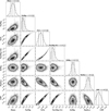 |
Fig. B.1 MCMC corner plot depicting the marginalized posterior distributions of the model parameters derived from the two-layer interior model for Kepler-10 b, including its mass, radius, bulk molar ratios (Fe/Mg, Si/Mg, and Fe/(Mg+Si)), iron-mass fractions, and CMF. The median values and the ±1σ uncertainties are represented by dashed lines. |
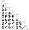 |
Fig. B.2 MCMC corner plot depicting the marginalized posterior distributions of the model parameters derived from the three-layer interior model for WASP-47 e, including its mass, radius, WMF, bulk molar ratios (Fe/Mg, Si/Mg, and Fe/(Mg+Si)), iron-mass fractions, and CMF. The median values and the ±1σ uncertainties are represented by dashed lines. |
All Tables
MCMC analysis of the 17 low-density exoplanets using the three-layer interior model.
All Figures
|
Fig. 1 Sample of selected exoplanets with radius measurements plotted as a function of mass and equilibrium temperature. Different colors denote the equilibrium temperature, Teq, of planets (zero albedo assumed). Dashed blue, light blue, and red lines, respectively, represent the M–R curves for pure-silicate, Earth-like, and pure-iron planets, derived by the interior model calculations. Critical masses of super Mercuries are labeled with dashed orange lines as a function of planetary radii, MSM = [0.25 + 0.87(R/R⊕)4.2]M⊕ (Unterborn et al. 2023). |
| In the text | |
|
Fig. 2 Stellar elemental ratios [Fe/Mg] and [Si/Mg] from three data sources: Brinkman et al. (2024, 2025) (red), Adibekyan et al. (2012b, 2021) (blue), and Brewer & Fischer (2018) (yellow). |
| In the text | |
|
Fig. 3 Iron-mass fractions of the 60 rocky exoplanets versus metal-licities [Fe/H] of their host stars. The iron-mass fractions are inferred through the MCMC method combined with the two-layer interior model. |
| In the text | |
|
Fig. 4 Comparison of the CMF of the rocky exoplanets with the equivalent stellar CMFstar. The CMFstar values were calculated from the Fe/Mg ratio of the host stars using Eq. (7) with the Earth-like mantle composition [Si/Mg = 0.96, Al/Mg = 0.09, Ca/Mg = 0.07, and assuming no iron in the mantle, fFeo = 0 (Adibekyan et al. 2021; Brinkman et al. 2024)]. The rocky planets depicted by thin rhombuses are classified as super-Mercuries, while those illustrated with circles are identified as super-Earths. Solid and dashed black lines denote the ODR and OLS fits to the sample of the super-Earths, respectively. |
| In the text | |
|
Fig. 5 Direct comparison of the iron-mass fractions (a) and the bulk molar ratios Fe/(Mg+Si) (b) of the 32 rocky exoplanets and their host stars. The compositions of the rocky exoplanets were inferred through the MCMC method combined with the two-layer interior model, whereas the compositions of the corresponding host stars were derived from the stellar elemental abundance ratios. |
| In the text | |
|
Fig. 6 Comparison of the stellar ages derived through isochrones in this work with those determined by Weeks et al. (2025). |
| In the text | |
|
Fig. 7 Magnesium abundance [Mg/Fe] of the host stars as a function of the stellar age. Different colors indicate the metallicity, [Fe/H], of the host stars. |
| In the text | |
|
Fig. 8 Iron-mass fractions of the rocky exoplanets versus the ages of their host stars. The ages of FGK stars (denoted by circles) were determined through isochrones, while the ages of M dwarfs (denoted by inverted triangles) were derived from the previous works. |
| In the text | |
|
Fig. 9 Effects of the model assumptions and statistical methods: the CMF results of Brinkman et al. (2024, 2025) that were computed from the best literature values for planet mass and radius (a), the median of the CMF posterior distribution (b), and the optimal CMF that corresponds to the case in which the likelihood function reaches its minimum value in the MCMC chain (c). For the purpose of direct comparison, the planet samples selected here are consistent with Brinkman et al. (2024, 2025). |
| In the text | |
|
Fig. 10 Variations in the mantle compositions of Brinkman et al. (2024, 2025) and the present work. The mantle compositions are characterized by the molar ratios of Fe/Mgmantle and Si/Mgmantle. The fixed mantle composition from Brinkman et al. (2024, 2025) is denoted by blue pentagrams, whereas the mantle compositions from our optimal CMF samples are illustrated as orange circles. |
| In the text | |
|
Fig. 11 Same as Figure 4, but with the equivalent stellar CMFstar values calculated using the reduced abundance uncertainty (σ[X/H] = 0.025 dex). For comparison, the ODR (solid orange) and OLS (dashed orange) fits from Figure 4 are also shown. |
| In the text | |
|
Fig. 12 MCMC posterior probability distributions for the mass and radius of WASP-47 e, derived from the two-layer model (a) and from the three-layer model (b). The median values, along with the ±1σ uncertainties, are depicted using dashed lines. The observed mass and radius are indicated by red lines. |
| In the text | |
|
Fig. B.1 MCMC corner plot depicting the marginalized posterior distributions of the model parameters derived from the two-layer interior model for Kepler-10 b, including its mass, radius, bulk molar ratios (Fe/Mg, Si/Mg, and Fe/(Mg+Si)), iron-mass fractions, and CMF. The median values and the ±1σ uncertainties are represented by dashed lines. |
| In the text | |
|
Fig. B.2 MCMC corner plot depicting the marginalized posterior distributions of the model parameters derived from the three-layer interior model for WASP-47 e, including its mass, radius, WMF, bulk molar ratios (Fe/Mg, Si/Mg, and Fe/(Mg+Si)), iron-mass fractions, and CMF. The median values and the ±1σ uncertainties are represented by dashed lines. |
| In the text | |
Current usage metrics show cumulative count of Article Views (full-text article views including HTML views, PDF and ePub downloads, according to the available data) and Abstracts Views on Vision4Press platform.
Data correspond to usage on the plateform after 2015. The current usage metrics is available 48-96 hours after online publication and is updated daily on week days.
Initial download of the metrics may take a while.