| Issue |
A&A
Volume 704, December 2025
|
|
|---|---|---|
| Article Number | A56 | |
| Number of page(s) | 14 | |
| Section | Atomic, molecular, and nuclear data | |
| DOI | https://doi.org/10.1051/0004-6361/202556786 | |
| Published online | 03 December 2025 | |
Infrared optical constants and band strengths of interstellar ice analogues: H2O:CO2 and H2O:CO2:CO mixtures at 10 K
1
Instituto de Estructura de la Materia, IEM-CSIC,
Calle Serrano 121,
28006
Madrid,
Spain
2
Institut des Sciences Moléculaires d’Orsay, UMR8214, CNRS, Université Paris-Saclay,
91405
Orsay,
France
3
CNRS, Aix-Marseille Université, Laboratoire PIIM,
Marseille,
France
★ Corresponding authors: This email address is being protected from spambots. You need JavaScript enabled to view it.
Received:
8
August
2025
Accepted:
24
September
2025
Abstract
Context. The high-quality infrared spectra of interstellar ices provided by the James Webb Space Telescope have evinced the need for accurate infrared (IR) optical constants of ice mixtures that could be used to model the observed band profiles including scattering and absorption contributions.
Aims. This article aims to provide IR optical constants and band strengths of ice mixtures containing H2O, CO2, and CO with mixing ratios comparable to those observed in interstellar ices, particularly in cold molecular clouds.
Methods. Single species ices of H2O, CO2, and CO as well as ices of binary H2O:CO2 and ternary H2O:CO2:CO mixtures were produced via background deposition on a cold substrate at 10 K. Visible refractive indices (at 633 nm) were retrieved from double interferometry measurements during ice growth. Ice densities were estimated using the Lorentz-Lorenz relation. The IR spectra (5000500 cm−1) of pure species and mixtures were employed to derive band strengths and optical constants. The optical constants were derived using a code based on the Kramers-Kronig causal relation and on Fresnel coefficients.
Results. The intensity of the imaginary part, k(ν), of the IR refractive index of porous single-species ices grown in this work is smaller than that of more compact ices available in the literature. Significant changes are observed in the optical constants of the mixtures as a function of mixing ratio. In general, the k(ν) intensity of a given IR band follows the evolution of the partial molecular density of the band carrier. The nature of intermolecular interactions and the ice morphology also affect the profile and intensity of the reported optical constants, but the various effects cannot be easily disentangled. The IR band strengths of some of the strongest H2O and CO2 absorptions were found to vary by as much as 25% in some of the binary and ternary mixtures with respect to those of the pure species ices.
Key words: astrochemistry / ISM: molecules
© The Authors 2025
 Open Access article, published by EDP Sciences, under the terms of the Creative Commons Attribution License (https://creativecommons.org/licenses/by/4.0), which permits unrestricted use, distribution, and reproduction in any medium, provided the original work is properly cited.
This article is published in open access under the Subscribe to Open model. This email address is being protected from spambots. You need JavaScript enabled to view it. to support open access publication.
1 Introduction
Ices are widespread in dense regions of the interstellar (IS) medium (see Boogert et al. (2015) and references therein). They form mantles on dust grains in molecular clouds and protostellar envelopes, play a key role as a reservoir for some of the most common elements, and serve as a site for interstellar chemistry. They have long been observed in absorption against infrared (IR) sources either embedded in clouds or behind them. A wealth of data from Earth-based or airborne observatories (Willner et al. 1982; Lacy et al. 1984; Brooke et al. 1999) and space telescopes such as ISO (Gibb et al. 2004; van Dishoeck 2004; Dartois 2005), Spitzer (Knez et al. 2005; Oberg et al. 2011), AKARI (Shimonishi et al. 2010; Aikawa et al. 2012; Noble et al. 2013), and JSWT (McClure et al. 2023; Yang et al. 2022; Sturm et al. 2023; Dartois et al. 2024; Noble et al. 2024; Rocha et al. 2024; Smith et al. 2025) have revealed that the main ice species are H2O, CO2, CO, CH3OH, CH4, and NH3. Small amounts of OCS and OCN− have also been detected, and the presence of other molecules has been tentatively suggested (Boogert et al. 2015). Among these molecules, H2O, CO2, and CO are by far the dominant ice components across the various IS environments, including low- and high-mass protostars and quiescent clouds (Oberg et al. 2011). They determine the bulk ice properties and are implicated in the formation of more complex molecules. Work by many research groups over the years has led to a global picture, albeit with open questions, of the formation and evolution of these molecules on the dust grains (Oberg et al. 2011; Boogert et al. 2015). H2O, the major ice species, is observed in cold cores for visual extinctions, Aν, larger than approximately 1.6 mag. It is believed to form through a barrierless hydrogenation of atomic oxygen on the grains (Furuya et al. 2015; Ruffle & Herbst 2000). The process is aided by the fast surface diffusion of H even at the very low temperatures (approximately 10 K) of dense clouds. Other routes involving the hydrogenation of O2 and O3 are also possible (Ioppolo et al. 2008). CO is formed in the gas phase and accretes thereafter onto the grains. It is observed for Aν larger than ≈ 3 mag. For very high gas densities, most of the CO condenses swiftly and is depleted from the gas phase (Caselli et al. 1999; Jorgensen et al. 2005). This pronounced increase in CO ice (Pontoppidan 2006), often known as catastrophic freeze-out, can form an apolar layer over the preexisting polar water-rich ice. Evidence for this layered structure comes from observed differences in CO and CO2 band profiles sensitive to the molecular surroundings (Ehrenfreund et al. 1997; Boogert et al. 2015). Entrapment or migration of some CO into the water-rich ice could account for a polar CO component in astronomical observations (Tielens et al. 1991). CO2 is observed with a threshold Aν larger than ≈ 1.6 mag, which suggests that its formation is linked to that of H2O. The surface reaction of CO with OH radicals was proposed as a possible source of CO2 in the water-rich ice (Oba et al. 2010; Ioppolo et al. 2011; Noble et al. 2011). A further increase in CO2 ice was observed upon CO freeze-out (Pontoppidan 2006), pointing to additional CO2 production pathways in the CO apolar medium (Garrod & Pauly 2011). However, the mechanisms of CO2 ice production are still debated (see Clément et al. (2023) and references therein). In the transition from dense clouds to protostars, the primary ices undergo desorption, segregation, crystallisation, and chemical reactions that change their composition and morphology, but H2O, CO2, and to a large extent CO are still the dominant components (Oberg et al. 2011; Boogert et al. 2015; McClure et al. 2023; Smith et al. 2025).
Interstellar ice appears inside molecular clouds before the onset of star formation. Until recently, studies of the chemical composition of cloud ices based on IR absorption against background stars were limited to regions with Aν < 50 mag (Knez et al. 2005; Boogert et al. 2015) due to the faintness of the stars for larger visual extinctions. These observations were likely biased towards the brightest individual lines of sight of single clouds. However, access to much denser regions and thus a more detailed investigation of pristine ices is now possible thanks to the high sensitivity and spectral resolution of the James Webb Space Telescope (JWST). Using a combination of the MIRI, NIRCam, and NIRSpec instruments of JWST, McClure et al. (2023) have reported ice inventories in the Chamaeleon I molecular cloud towards two highly extinct background stars labelled NIR38 and J110621, which correspond to very dense lines of sight (estimated pre-JWST of Aν = 60 mag and 95 mag, respectively). Besides the three main components H2O, 12CO2, and 12CO, weaker bands of 13CO2, 13CO, and OCN− and OCS transitions were clearly identified. Other weak absorption features suggest the possible presence of NH+4, CH4, NH3, and of functional groups of more complex organic molecules. A tentative detection at 2.7 μm of OH dangling bond (dB) features, which are characteristic of not fully coordinated water molecules (Buch & Devlin 1991; Rowland et al. 1991), was confirmed in a subsequent work by Noble et al. (2024). In their very recent publication, Smith et al. (2025) extend the study of Chamaeleon I ices by presenting co-spatial maps of H2O, CO2, and CO derived from observations towards 44 lines of sight with a median resolution of 2000 au. The maps illustrate the simultaneous formation of CO2 and H2O ice and suggest the onset of additional CO2 formation within CO ice at higher densities. There are appreciable local variations in the relative abundances of H2O, CO2, and CO, whose significance is yet to be explored.
The deepest absorption bands measured towards Chamaeleon I exhibit ice band profile distortions due to light scattering. A model of the spectral profiles towards NIR38 and J110621 including scattering effects (Dartois et al. 2024) showed that the H2O, CO2, and CO band profiles are associated with a growth of the grains up to the micrometer size. The modelling required a definition of grain shapes and sizes as well as the composition, structural arrangement, and optical constants of the refractory and ice phases of the grain (Dartois et al. 2022). The initial spectral evaluation of the chemical composition (McClure et al. 2023) disregarded scattering effects, while the model of Dartois et al. (2024) included optical constants corresponding to two CO populations, a fraction of CO mixed with H2O and a fraction of pure CO, in order to account for the observed band profiles.
It has often been assumed that interstellar ices are mostly compact. This assumption was long supported by the nondetection of the OH dangling bond features and by the fact that the water ice formed in the laboratory through surface reactions was found to be compact (Oba et al. 2009). Laboratory experiments further showed that the interaction of water ice with high energy ions (Palumbo 2006; Raut et al. 2007; Dartois et al. 2013; Mejia et al. 2015), UV photons (Palumbo et al. 2010), and H atoms (Accolla et al. 2011) leads to a drop in the dB intensity, which in some of these references is shown to be associated with a decrease in porosity. The recent detection of dB bands in Chamaeleon I (Noble et al. 2024) mentioned above provides a tracer that will allow for the testing of whether porous ice can be observed in some environments. Nonetheless, dB features cannot be easily correlated with porosity in a quantitative way in complex ice mixtures since their presence and intensity are highly dependent on the scale of the pores and on the physical and chemical interactions in the ice and specifically on the degree of mixing with molecules other than H2O. On the other hand, the absence of dB bands does not fully exclude porosity (Raut et al. 2007; Isokoski et al. 2014). In any case, the porosity of a given ice sample is reflected in its optical constants, and the derivation or modelling of porosity-dependent optical constants (Bossa et al. 2014, 2015) for ice mixtures of interest should be of great help for the interpretation of astronomical spectra.
In this work we present a study of IR spectra, band strengths, and optical constants of binary and ternary mixtures of the dominant IS ice components (H2O, CO2, CO) at 10 K. The mixture proportions were chosen to cover the range of interest for the recent JWST observations of dense clouds, and we expect that the results will be of help in the interpretation and modelling of observational spectra. We focus on ices obtained in the laboratory through background gas deposition. Experimental mid-IR spectra, band strengths, and optical constants of unmixed ices of H2O, CO2, and CO have been reported in the literature by many groups (see e.g. Hagen et al. (1981); Hudgins et al. (1993); Ehrenfreund et al. (1997); Elsila et al. (1997); Baratta & Palumbo (1998); Palumbo et al. (2006); Mastrapa et al. (2009); Gerakines & Hudson (2015, 2020); Rocha et al. (2022); Gerakines et al. (2023). Many of these data are archived in databases.1 Similar spectral information is also available for mixed ices of H2O, CO2, and CO (see e.g. Sandford et al. (1988); Sandford & Allamandola (1990); Accolla et al. (2011); Gerakines et al. (1995); Ehrenfreund et al. (1997); Elsila et al. (1997); Bernstein et al. (2005); Oberg et al. (2007); Bossa et al. (2014); Baratta & Palumbo (2017); He et al. (2018) and references therein). The data on these ice mixtures comprise a wide variety of ice temperatures and mixture proportions, but in general, they do not present a systematic study of mixing ratios, and sometimes they are restricted to a small spectral interval. Only a few of them have been included in databases. A full discussion of the extensive literature on ice mixtures of H2O, CO2, and CO is beyond the scope of the present work, but the results relevant to this study are commented on in the text.
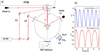 |
Fig. 1 a) Scheme of the experimental setup. b) Laser interference signal recorded at two incidence angles, α = 1.3 deg and β = 76. 5 deg, during H2O:CO2:CO 100:26:40 ice growth at 10 K at a constant deposition rate of 4 μm/h. |
2 Experimental part, calibrations, and methodology
2.1 Experimental setup
Figure 1a shows a scheme of the experimental setup. Ice layers were grown through background vapor deposition in a high vacuum cylindrical chamber that can be evacuated to a base pressure of 10−8 mbar with a turbomolecular pump (Pfeiffer HIPace 300). The chamber contains a closed-cycle He cryostat (ARS DE204B) and is coupled through KBr windows to a Fourier transform infrared spectrometer (Bruker Vertex 70). The gases were introduced into the chamber through independent inlets. Distilled water, subjected to three freeze-pump-thaw cycles, was placed in a thermal bath to stabilise the vapor pressure. Water vapor was introduced in the chamber through a calibrated needle valve. Two additional independent lines, equipped with mass flow controllers (Alicat scientific), were used for CO2 (Alphagaz 99.98) and CO (Alphagaz 99.997) gases. The reproducibility of the gas flows was very good, with variations below 5% between different experiments. The three inlet ports are situated in the chamber wall about 12 cm below the bottom of the cold head of the cryostat, to ensure a homogenous pressure filling of the chamber volume and background deposition of the ices. An IR transparent substrate was placed in a copper sample holder in good thermal contact with the cold tip of the cryostat. On one side, the sample holder has an open cylinder (23 mm long, 10 mm diameter) perpendicular to the substrate surface. This arrangement allows for the passage of the IR beam but prevents gas condensation on this face (which we call the back side) of the substrate (see sketch in Fig. 1a). Geometric calculations indicate that the fraction of gas deposited on the back side should be less than 1% (see for instance Herczku et al. (2021) ). The deposition pressures used in our experiments range between 1 and 4 × 10⁻⁶ mbar. Two silicon diodes positioned at the end of the cold finger and at the bottom of the sample holder are used to measure the substrate temperature, which is kept at 10 K in all the experiments. Both KBr and Si substrates were used in the experiments. In particular, the double interferometry measurements for the determination of visible refractive indices (see next subsection and Fig. 1) were performed with a Si substrate. In these measurements, two beams from a He-Ne laser were reflected on the Si surface at incidence angles α = 1.3 deg and β = 76.5 deg. When ices were grown on the KBr substrate, the interference pattern was recorded only at the larger incidence angle (≈76 deg) because the signal of the laser at near normal incidence was too weak. Normal incidence transmission absorption spectra in the mid-IR spectral range (5000 - 500 cm−1) were recorded during ice growth. Spectra were taken every 30 seconds, with 2 cm−1 spectral resolution and accumulating 50 scans. Under these conditions, the acquisition of each spectrum takes 15 s. Two sets of experiments were performed growing the same ice mixtures, one on the Si substrate and the other on the KBr substrate. Although our experimental configuration allows us to record IR spectra while performing the double laser interference experiments, the Si substrate causes larger distortions in the absorption band profiles due to its higher refractive index. For that reason, we decided to repeat the experiments by growing the same ices on a KBr window. The differences in the mixing ratios of the corresponding samples in the Si and KBr experiments were in the few percent range.
Measured visible refractive indices, n633, and estimated densities, ρ, of the ices of H2O, CO2, and CO.
2.2 Visible refractive indices and film thickness
We performed two-angle laser interferometry to measure the refractive index of the ice layers at the He-Ne laser wavelength (λ= 632.8 nm), n633, using the experimental geometry depicted in Figure 1a. Two beams, from the same intensity-stabilised He-Ne laser, hit the ice at angles of α = 1.3 degrees and β = 76.5 degrees with respect to the surface normal, as determined from high resolution photogrammetric analysis. From the angles (α,β) and the period of the two interference patterns recorded during ice growth, the ice refractive index is obtained via the expression (Tempelmeyer & Mills 1968; Domingo et al. 2021)
 (1)
(1)
where γ = τα/τβ is the ratio of the periods τα and τβ of the two interference patterns seen at angles α and β, respectively. The estimated uncertainty in the refractive index, n633, is below 1%. It is derived from the errors in the angles (0.1 deg) and the time period (below 1%). Figure 1b shows an example of the He-Ne interferences obtained for a ternary ice mixture at the two incidence angles. The n values obtained in the present experiment for the ices of the pure species at 10 K are listed in Table 1. They are in good agreement with the refractive indices from other laboratories for ices of the same substances obtained by background vapor deposition at T ≤ 20K, nH2O = 1.19-1.2 (Brown & George 1996; Dohnálek et al. 2003; Isokoski et al. 2014), nCO2 = 1.21-1.27 (Schulze & Abe 1980; Wood & Roux 1982; Domingo et al. 2021), nCO = 1.27-1.28 (Roux et al. 1980; Luna et al. 2022).The thickness of a given ice layer was determined from the corresponding deposition time and growth rate, which was kept constant during deposition. The growth rate was easily derived from the measured n633 refractive index by considering that the increase in the thickness of the ice during one interference period, τθ, corresponding to a given incidence angle, θ, is given by
 (2)
(2)
where λ is the He-Ne laser wavelength, n is the refractive index of the ice, and θ is the angle of the incident laser beam with respect to the surface normal. Note that in our experiments, the angle θ in Eq. (2) can either be α or β, and the thickness growth rate, r, can be expressed as
 (3)
(3)
where Δx is the increase in thickness and Δt is the corresponding deposition time. The recorded interference patterns were very regular, as shown in Fig. 1b. Nevertheless, in order to average out possible small differences and increase accuracy, several interference periods were used in the calculation of growth rates. Typical growth rates in the present experiments range from approximately 1-5 μ h−1.
2.3 Preparation of ice mixtures, pressure calibration, and densities
As indicated above, ice mixtures of H2O, CO2, and CO were prepared by simultaneous deposition of two or three of these species from the gas phase on the cold (10 K) substrate. Each species was dosed into the chamber via an independent dosing line. Assuming a sticking coefficient of 1 for the three species, the proportion of the different molecules in the deposited ices can be estimated from gas-kinetic theory. For a given species, the number of molecules deposited in an ice sample is readily derived from the molecular flux to the surface, Φ (molec cm−2 s−1), which is given by the collision frequency per unit surface area:
 (4)
(4)
where nm is the molecular density, <v> is the average molecular velocity, P is the gas pressure, m is the molecular mass, Tg is the gas temperature, and k is Boltzmann’s constant. In all the experiments the deposition chamber was kept at room temperature (Tg = 298 K) so that  , and the desired ice mixtures were prepared by setting the partial pressures of the various components. Gas pressures in the deposition chamber were measured with a Bayard-Alpert (BA) hot cathode gauge (Leybold ITR 090). A calibration of the gauge, based on the interference measurements, was performed for each of the individual species. The gauge was calibrated by comparing the gauge reading with the gas pressure corresponding to the observed growth rate as measured from the interference pattern (Eq. (3)):
 (5)
(5)
where ρ is the bulk mass density of the deposited ice. The ice densities were estimated as indicated below and are listed in Table 1. A calibration factor, fi, was obtained for each species from Pi = fiPBA,i, where PBA,i is the BA gauge reading for species i, and Pi is the corresponding pressure given by Eq. (5). The calibrated gauge was used in turn to calibrate the needle valve (H2O) and flow controllers (CO2, CO) employed for the selection of the partial pressures leading to the desired ice mixtures. An independent procedure based on the determination of the gas flow to the chamber and on the measurement of the pumping speed of the turbomolecular pump for each gas (see Maté et al. 2003) was also used to calibrate the BA gauge. The calibration factors, fi, derived for H2O and CO2 were found to be coincident (differences less than 3%) with those obtained from the interference method just described. The fco factor was ≈ 10% higher. We could not determine the reason of this discrepancy. Throughout this work we have used the pressure calibration derived from the interference measurements. This procedure is more usual in the astrochemical literature and thus more suitable for comparison with other works. In any case, the differences between the two methods would not significantly modify the conclusions. Gas flow (pressure) reproducibility was better than 5%, and the stability during the deposition time (30-60 min) was better than 2%. To avoid saturation of the mid-IR absorption features, the ice thickness employed to determine optical constants and band strengths was kept below 800 nm.
The densities of the individual H2O, CO2, and CO ices deposited at 10 K were estimated from the measured refractive indices by using the Lorentz-Lorenz relation, which is known to hold for these species (see for instance Brown & George (1996); Westley et al. (1998); Loeffler et al. (2016); Domingo et al. (2021); Luna et al. (2022):
 (6)
(6)
where n is the visible refractive index (in this study n633), NA is Avogadro’s number, ρ is the ice density (g cm−3), M is the molar mass (g mol−1), α is the polarisability volume (Å3), and L (cm3 g−1) is the Lorentz-Lorenz coefficient (specific refraction). The values of the polarisability used in equation (6) and the resulting L coefficients and densities are given in Table 1.
The polarisabilities listed in Table 1 correspond to experimental literature values from ice samples. Gas-phase polarisabilities for these molecules have similar values. A compilation (Hohm 2013) containing data from different experimental techniques gives α = 1.42-1.45 Å3 for H2O, α = 2.59-2.65 Å3 for CO2, and α = 1.82-1.97 Å3 for CO. The uncertainties in the densities listed in the table were calculated by propagating the errors in the refractive indices and polarisabilities assuming an uncertainty of 0.03 Å3 in the polarisability values.
The densities given in Table 1 are similar to those measured by other groups for ices of the same substances produced in a similar way, i.e. deposited from the background gas at temperatures ≤20 K: ρH2O = 0.6-0.63 g cm−3 (Brown & George 1996; Dohnálek et al. 2003), ρCO2 = 0.98-1.08 g cm−3 (Schulze & Abe 1980; Wood & Roux 1982; Domingo et al. 2021) and ρCO = 0.80-0.88 g cm−3 (Roux et al. 1980; Luna et al. 2022). The latter value has been recently brought into question by Gerakines et al. (2023), who measured a density ρco = 1.029 g cm−3 for CO directionally deposited at 25 K. Among other things, these authors noted that the application of the Lorentz-Lorenz equation with the densities of Roux et al. (1980) or Luna et al. (2022) leads to a polarisability value 20% in excess of the experimentally measured one. Our ρco = 0.91 g cm−3, estimated with the Lorentz-Lorenz relation using the experimental polarisability (Ron & Schnepp 1967) and our measured refractive index, is close to the value of ρCO = 0.85 g cm−3 obtained by Luna et al. (2022) at 13 K. The discrepancy of the present values with those of Gerakines et al. (2023) is not surprising since the deposition methods are different and thus the ices have likely different morphologies.
The densities of the deposited ice mixtures could not be derived from the Lorentz-Lorenz relation, since their polarisabilities are not known, but they can be estimated from the flux of the various molecules onto the substrate that can be calculated with equation (4) using the calibrated partial pressures. Adding up the contribution of each species, it is possible to estimate the total mass column density of the mixture, Nρmix, (g cm−2). The ice layer thickness of the mixture, lmix, is known from the interference measurements. The density (g/cm3) is then calculated as
 (7)
(7)
where φi (molec cm−2 s−1) is the flow of species i to the substrate, NA is Avogadro’s number, and r (cm/s)=Δx/Δt is the thickness growth rate (Eq. (3)) determined from the interference experiments. The uncertainties in the mixture densities derived with this equation are estimated to be less than 7% considering the uncertainties in the fluxes (below 5%) and in the growth rate (2%). The partial density of each species in the mixture is given by
 (8)
(8)
where Mi is the molar mass of species i.
2.4 Determination of infrared optical constants
To determine mid-IR optical constants, we employed the freely available software provided by Gerakines & Hudson (2020). The method is analogous to that used by Hagen et al. (1981) and Hudgins et al. (1993) to extract optical constants of astrophysical relevant ices from a single IR transmittance spectrum of an ice film deposited in an infrared transparent substrate. The code introduces modifications to the standard algorithm employed by Hudgins et al. (1993) to avoid convergence issues. The program allows the retrieval of IR optical constants of ice layers grown on one side of an IR transparent substrate from their IR absorbance (or transmittance) spectrum recorded at normal incidence. The input parameters are the baseline corrected (overall slope and interference fringes removed) IR absorbance (or transmittance) spectrum, the refractive index of the ice in the visible region, the thickness of the ice layer, and the optical constants of the IR transparent substrate in the same wavelength range as the ice IR spectrum. In the present work, the optical constants of KBr were taken from Li (1976). The equations, based on Fresnel coefficients, employed to simulate the transmitted intensity through a three-layered system vacuum/ice/substrate (see, for example, Eqs. (2), (4), (5) in Hudgins et al. (1993) simulate not only the absorptions but also the interferences due to reflections at the multiple interfaces. In the raw experimental transmission spectra, these interferences might appear with periods and amplitudes slightly different than those simulated by the program. The reasons for these discrepancies are small effects including scattering loses, multiple internal reflections, or small errors in the alignment of the IR beam perpendicular to the ice deposition surface. Therefore, to facilitate the fitting procedure, Hudgins et al. (1993) and later Gerakines & Hudson (2020), chose to first baseline correct the recorded IR spectrum and then add an interference baseline simulated considering the thickness of the ice layer. This procedure facilitates the convergence when comparing simulated and experimental spectra.
To mitigate the effect of the uncertainties in the ice layer thickness determination and manual baseline subtraction, in the present work the optical constants were derived for five distinct spectra of samples with the same ice mixture, but deposited with different thicknesses. The derived optical constants of that particular ice mixture were obtained by averaging the five sets of optical constants (see Subsection 3.2.3).
2.5 Band strength determination
The integrated band strength for a band of species i can be obtained from the imaginary part of the refractive index as
 (9)
(9)
where ρi is the partial density of the species i:H2O, CO2 or CO; ν is the wavenumber; and k(ν) is the imaginary part of the refractive index of the ice mixture. It is also possible to obtain an effective band strength, A′i, from the absorbance (log10) spectrum and the column density of absorbing species using
 (10)
(10)
where the numerator is the integral of the band in the absorbance spectrum, Abs(ν), and Ni is the column density of species i. This expression can be rearranged as
 (11)
(11)
The integrated band intensity can be plotted versus deposition time for a constant flux, φi (molec cm−2 s−1), of species i (H2O, CO2 or CO). Then, from the slope of the linear fit, the effective band strength is extracted. This method was employed to obtain the A’ values of the various H2O, CO2, and CO IR absorption bands in pure ices and mixtures.
3 Results
3.1 Refractive indices at λ = 633 nm and densities
Table 2 lists the ice mixtures used for the derivation of refractive indices and densities. The refractive indices at the He-Ne laser wavelength were derived from the double interferometry measurements described in Section 2.2, and the densities of the ice mixtures were obtained with equation (7). These data are represented in Fig. 2. Refractive indices and densities for H2O:CO2 mixture ratios different from those studied here can be determined by interpolation within the studied range.
An additional column with a ‘nominal mean density’ has been added to Table 2 to allow for comparison between the ice samples. It was obtained by averaging the ice densities of the pure species with the molecular proportion of the individual components in each mixture. The physical mixture densities are always higher than the nominal mean densities indicating that co-deposition leads to a certain degree of ice compaction and suggesting that, in the mixed ices, CO and CO2 induce changes in the ice structure, possibly leading to a reduction in the global extent of hydrogen bonding. The differences in ice morphology between directional and background deposition are probably smaller in the case of ice mixtures.
Molecular mixing ratios; refractive indices at λ = 632.8 nm; n633 densities, p; and estimated nominal mean densities, ρmn (see the text).
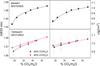 |
Fig. 2 Refractive indices (at λ = 632.8 nm) and densities of H2O:CO2 and H2O:CO2:CO ice mixtures grown by background vapour deposition at 10 K. Lines are drawn to guide the eye. |
3.2 Infrared spectra and optical constants
In this section we comment on the main IR spectral absorptions and on IR refractive indices (the so-called optical constants) of pure ices and mixtures. The complex IR refractive indices for all the ices studied in this work can be found in the Zenodo repository (see Data availability section).
3.2.1 Infrared spectra
Figure 3 shows the evolution of the main IR absorption bands for the studied ice mixtures. The mixing ratios cover a wider range, as can be seen in Table 2, but for clarity a selection of mixtures has been displayed. The band profiles of the pure H2O, CO2, and CO ices are distorted by the presence of the other mixture components that can form different types of complexes in the resulting ice matrices. These changes have been observed and discussed in previous works (Ehrenfreund et al. 1997; Sandford et al. 1988). They are just briefly described at this point. In panel (a) the broad OH stretching band at ≈3298 cm−1 corresponds to amorphous water and its overall shape is not much affected in the mixtures. With increasing CO2 content, the peak shifts from ≈ 3298 cm−1 to ≈ 3350 cm−1 and, for CO2:H2O ratios higher than 0.3, a smooth shoulder appears at approximately 3240 cm−1. Small combination bands of CO2 and a dB peak near 3650 cm−1, characteristic of OH interactions with CO2 and CO (Palumbo 2006; Noble et al. 2024), can be seen in the blue wing of this band.
Panel (b) displays the band of the ν3 antisymmetric stretching of CO2. For pure CO2, it is broad, with a peak (2345 cm−1) and a shoulder (2328 cm−1) that is probably caused by a mixture of crystalline and amorphous CO2 (see discussion below). The presence of crystalline ice in the solid is also reflected in the double peak observed for the corresponding CO2 ν2 bending mode (panel e). The ν3 band is narrower and more symmetric in the dilute mixtures (CO2:H2O below 0.2), but it broadens and becomes asymmetrical with growing CO2 proportion. The double peak (near 660 cm−1, 655 cm−1) and the definite structure of the bending mode in panel (e) are also lost in the mixtures, where the band becomes smooth with a broad maximum at 655 cm−1 and a slow decaying red wing. Panel (c) shows the evolution of the stretching mode band of carbon monoxide. The spectrum of pure CO ice, which for our experimental conditions corresponds most likely to crystalline α CO (see below), shows a narrow band peaking at 2139 cm−1 . In all the mixtures, the band broadens and extends asymmetrically towards the blue wing. In the two mixtures containing less CO2 (CO2:H2O below 20%) a shoulder is visible at 2150 cm−1 . In the two mixtures containing more CO2 (CO2:H2O larger than 0.5) the shoulder is blurred within the slowly decreasing blue wing. The marked modification of the CO band in ice has received much attention since the earliest studies of CO:H2O ices. Sandford et al. (1988) attributed the peak at 2139 cm−1 to a substitution of an H2O molecule for a CO molecule in the ice matrix, and the shoulder at 2150 cm−1 to interstitial CO located within the pores of the amorphous water ice lattice. Hasegawa et al. (2024) have recently attributed the 2150 cm−1 shoulder to CO molecules hydrogen bonding to dangling OH through the carbon atom, and the 2139 cm−1 main peak to CO interacting with H2O molecules hydrogen bonded to other water molecules. Panel d) displays the spectral interval containing the ν2 bending (1650 cm−1) and νL libration (750 cm−1) modes of H2O ice. The ν2 band of pure water ice is asymmetric with an extended red wing that has been attributed to an overtone of the libration mode (Devlin et al. 2001; Oberg et al. 2007). In the mixtures the wide reward wing remains. With increasing CO2 content, the peak becomes sharper and shifts to lower wavenumbers (1643 cm−1 for CO2:H2O below 0.4) and the band decreases more abruptly on the reward side. For binary H2O:CO2 mixtures, Oberg et al. (2007) reported the presence of a second peak component at 1609 cm−1 that grows in intensity with increasing CO2 and becomes prominent for CO2:H2O lower than one. This component could be due to overlapping ν2 vibrations of water monomers, dimers, and small multimers separated from the hydrogen bonded network as the CO2 concentration increases. We have found no evidence for this second peak component in our experiments. The νL libration band of H2O, also shown in panel (d), is broad with a maximum at 750 cm−1. In the mixtures, the narrower CO2 bending mode band at 655 cm−1 is superimposed, but at first look no large changes are observed in the shape of the libration band as the mixing ratio varies. The CO2 bending mode band is shown in more detail in panel (e). As already mentioned, the main change observed is the disappearance of the double peak structure in the mixtures. The band maximum at 656 cm−1 becomes somewhat more pronounced in the mixtures with higher CO2 content.
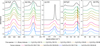 |
Fig. 3 Main mid-IR absorptions in pure ices and in binary and ternary mixtures: (a) OH stretching modes (ν1,ν3) of H2O; (b) antisymmetric stretching mode (ν3) of CO2; (c) stretching mode (ν) of CO; (d) bending (ν2) and libration (ν1) modes of H2O near 1650 and 750 cm−1, respectively, and bending mode (ν2) of CO2 near 657 cm−1 ; (e) enlargement of the ν2 mode of CO2. All bands of a given species presented in a panel correspond to the same number of molecules of that species. Specifically, in panels (a) and (d), NH2O = 4.8 × 10¹⁷ molecules cm−2; in panels (b) and (e) NCO2=1.7 × 10¹⁷ molecules cm−2 ; and in panel (c) NCO = 4.0 × 10¹⁷ molecules cm−2. |
3.2.2 Infrared refractive index. Pure species
In Fig. 4, the imaginary part, k(ν), of the IR refractive indices of pure H2O, CO2, and CO ices obtained in this work is compared to previous results from astrochemical databases. The upper panel of Fig. 4 corresponds to amorphous water ice at 10-30 K. In this work, water ice was grown via background deposition at 10 K and is porous. Previous water ice optical constants were derived from ices grown between 10 and 30 K by different kinds of directional deposition (Hudgins et al. 1993; Mastrapa et al. 2009; Rocha et al. 2022), and the resulting ices are expected to be more compact. The higher k values redward of 2000 cm−1 found by Mastrapa et al. (2009) might be due to different baseline corrections. The degree of ice compactness is reflected in k(ν), which is related to the attenuation of radiation in the medium and will be larger for more compact ices. This explains why the literature k(ν) values are higher than those reported in this work. To discount the effect of the differing density, the k(ν) from this work has also been scaled (dashed line) to the maximum of the 3292 cm−1 H2O band of Hudgins et al. (1993). An excellent agreement is obtained over most of the spectral range with a scaling factor 1.47, which corresponds roughly to the ratio of the densities of the compact ice of Hudgins et al. (1993) and the porous ice of our experiment. For this comparison we have assumed a density ρH2O of 0.94 g cm−3 for the compact ice of Hudgins et al. (1993) as expected for deposition along the surface normal (Dohnálek et al. 2003). However, the intensity of the libration (hindered rotation) band at 750 cm−1, which is more sensitive to the solid environment, remains smaller after the scaling. The intensity ratio between the libration and OH stretching bands can thus serve as an indication of ice porosity in pure water ice.
The middle panel of Fig. 4 displays the k(ν) for the ν3 stretching and ν2 bending modes of CO2 ice. There are appreciable differences in the band profiles derived by different groups. The lowest k(ν) are obtained for the present porous ices. They are closer to the results of Baratta & Palumbo (1998) than to the others. These authors also used background deposition. Some degree of directional deposition was used in the rest of the experiments. Except for the data of Gerakines & Hudson (2020), the ν2 bending band at 657 cm−1 shows a double peak usually taken as an indication of crystalline CO2 ice. The double peak is less pronounced in the present data and in those of Baratta & Palumbo (1998). The measurements of Gerakines & Hudson (2020) were carried out with a very low deposition rate (0.1 μm/h) and led to broader unstructured bands assigned to amorphous CO2. Gerakines & Hudson (2015) further argued that for the higher growth rates employed in most laboratories the energy released by condensation of room temperature CO2 molecules on the cold substrate would crystallise the forming ice even at 10 K, and thus the rest of the data shown would correspond to crystalline CO2. However, Escribano et al. (2013) and Baratta & Palumbo (2017) have shown that the double peak structure of the ν2 bending band is also obtained for growth rates below 0.1 μm/h at 10 K where no crystal formation is a priori expected. The most likely explanation for the variety of k(ν) is that the results from the various laboratories correspond to mixtures of amorphous and crystalline CO2 in diverse proportions. Crystallisation at about 10 K is probably very sensitive to the deposition rate and directionality and also to the ice thickness. The presence of amorphous CO2 in the ice sample of the present experiment is suggested by the small size of the splitting in the ν2 band and by the shoulder at about 2228 cm−1 in the ν3 band.
The lower panel of Fig. 4 shows the results for the stretching mode of CO ice. Again, the present k(ν) is similar to that of Baratta & Palumbo (1998), that corresponds to CO produced by background deposition. They are lower than the rest of the measurements where the ices were generated by directional deposition. The narrow CO absorption feature could be affected by the spectral resolution. The literature data shown were recorded with 1 cm−1 resolution, except for those of Baratta & Palumbo (1998) that used 2 cm−1. Since the main goal of our work is to provide optical constants of ice mixtures, in which the CO band is broader, we have worked with 2 cm−1 resolution in all the experiments. Therefore, this spectral resolution could contribute to the broadening of our CO band. As in the case of CO, Gerakines et al. (2023) have argued that deposition at the growth rates of most experiments should lead to crystalline ice even at very low temperatures. This argument is supported by the electron diffraction measurements of Kouchi (1990) who found that for deposition rates larger than 0.1 μm/h crystalline α CO is formed even at 10 K. Consequently, the data presented in Fig. 4 should correspond to α CO rather than amorphous CO ice. Gerakines et al. (2023) also recorded spectra of amorphous CO grown at a slow rate at 10 K that showed an appreciably broader ν CO band, but as far as we know no optical constants have been reported. Recent works by Kouchi et al. (2021b,a) have used transmission electron microscopy (TEM) and IR spectroscopy to investigate morphology and crystallisation in mixed ices of H2O, CO2, and CO deposited on refractory materials. From the results of their measurements, and considering the energy released in the condensation and reaction processes leading to IS ice formation, these authors concluded that, in a molecular cloud, amorphous CO2 should crystallise in 105 yr at 16 K, and amorphous CO in 103 yr at 10 K; therefore, the crystalline phases of these molecules could be expected in molecular clouds that have typical lifetimes of 107 yr. In fact, crystalline α CO is probably the dominant CO ice phase in IS environments including molecular clouds (Chiar et al. 1995; Pontoppidan et al. 2003; Boogert et al. 2015)
Crystalline CO2 is assumed to be present in the comparatively warm envelopes of young stellar objects (Gerakines et al. 1999; Pontoppidan et al. 2008; Yang et al. 2022) where the characteristic splitting of the ν2 mode has often been observed. In these environments, pure crystalline CO2 could segregate from the ice mixture. Note, however, that in some cases a splitting of the ν2 band could also be caused by the formation of CO2 dimers or intermolecular complexes with other molecules like CH3OH (Dartois et al. 1999; Klotz et al. 2004; Baratta & Palumbo 2017). The presence of crystalline CO2 in cold molecular clouds is not clear. The ice mantles in the Taurus molecular cloud (TMC) have been observed towards the background star Elias 16. Based on an analysis of the ν3 stretching band, Escribano et al. (2013) concluded that CO2 is likely crystalline, due to the absence of the 2228 cm−1 absorption feature characteristic of amorphous ice.
However, the splitting of the ν2 mode at approximately 655 cm−1–another indicator of crystallinity– was not observed in this source (Bergin et al. 2005). Unfortunately, the recent JWST observations of the Chamaeleon I molecular cloud (McClure et al. 2023; Smith et al. 2025) did not include coverage of the 655 cm−1 (15 μm) wavelength range. The absence of the splitting at 655 cm−1 among the non-thermally evolved clouds or some of the protostellar sources suggests that the CO2 is more often intermixed with other ices and/or in a non-crystalline form.
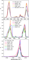 |
Fig. 4 Imaginary part, k(ν), of the refractive index (optical constant) of H2O (upper panel), CO2 (middle panel), and CO (lower panel) ices and comparison with literature values. The literature sources were the NASA and LIDA optical constants databases, a) Hudgins et al. (1993) b) Mastrapa et al. (2009), c) Rocha et al. (2022), d) Ehrenfreund et al. (1997), e) Baratta & Palumbo (1998), f) Gerakines & Hudson (2020), g) Elsila et al. (1997), h) Palumbo et al. (2006), i) Gerakines et al. (2023). |
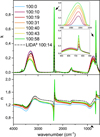 |
Fig. 5 Complex refractive indices of H2O:CO2 ice mixtures grown at 10 K. Solid lines, this work. Dashed line, LIDA database; a) Ehrenfreund et al. (1997). |
3.2.3 Infrared refractive index. Mixtures
Figure 5 displays the refractive index of the binary H2O:CO2 mixtures studied in this work. The k(ν) for the distinct H2O and CO2 bands follow the evolution of the relative mixture ratios. Increasing the proportion of CO2 leads to a decrease in the bands of H2O and vice versa, and the converse happens for the CO2 absorptions. Figure 5 also illustrates the good agreement between our data and the only k(ν) found for H2O:CO2 mixtures in the considered databases. It corresponds to a H2O:CO2 (100:14) mixture (Ehrenfreund et al. 1997). The k(ν) of the CO2 absorption bands nearly matches that of our (100:10) mixture (see inset in Fig. 5) and the OH bands are also very similar. Note that this good accordance is obtained despite the different ice formation methods: background deposition in the present study, and directional deposition in the work of Ehrenfreund et al. (1997). As noted in the previous discussion on ice densities, in co-deposited mixtures the highly porous structure of background deposited water is probably lowered by host molecules and a more compact ice morphology is obtained irrespective of the deposition procedure.
Figure 6 shows the refractive indices of ternary H2O:CO2 :CO mixtures. Unsurprisingly, the general trend is the same as in the binary mixtures, with higher k(ν) for the larger relative proportions of a given mixture component. The features of H2O are seen to stand out from the rest in the mixture with the highest water content. The left inset in the upper panel shows that the k(ν) for the ν3 absorption of CO2 does not depend of the amount of CO in the mixture and is just determined by the H2O:CO2 ratio. In contrast, the ν CO mode (right inset in the upper panel) depends both on the H2O:CO ratio, which determines mostly the relative intensity, and on the amount of CO2 that modifies the band shape. In the two mixtures with a H2O:CO2 (100:17) ratio, a shoulder towards 2150 cm−1 is clearly seen, whereas in those with more CO2, this shoulder is blurred and the CO peak blue shifted.
In general, the change in k(ν) for the various bands in the mixtures are expected to be largely due to changes in the partial densities of the band carriers, but the k(ν) can also be affected by the modification of molecular environments brought about by the mixing process. The two effects cannot be easily disentangled. We extend the discussion on mixing effects in the next section dedicated to band strengths. The main sources of error in the optical constants are the uncertainties in the ice layer thickness, the refractive indices at 633 nm (n633), and in baseline subtraction. We estimate the error in the ice layer thickness to be approximately 2% and less than 1% for n633. To reduce the effect of uncertainties in the layer thickness and baseline subtraction, we averaged the optical constants derived from spectra of five different layers. The standard deviation of that set of measurements was below 4%. Overall, we estimate an uncertainty of ≈5% in the optical constants.
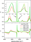 |
Fig. 6 Complex refractive index of H2O:CO2:CO ice mixtures grown at 10 K. The left inset in the upper panel corresponds to the ν3 mode of CO2 (2343 cm−1) and the right inset to the CO stretching mode (2140 cm−1). |
Infrared band strengths of pure H2O, CO2, and CO ices.
Comparison of the band strengths of this work with literature results.
3.3 Infrared band strengths
3.3.1 Pure species
The effective band strengths, A’, obtained from the absorbance spectra (Eq. (10)) of pure H2O, CO2, and CO ices grown via background deposition at 10 K are presented in Table 3. They are compared with the A band strengths derived from their k refractive indices using equation (9). The agreement between the two sets of band strengths is in general very good.
The present A’ values for the main absorption bands of H2O, CO2, and CO are compared in Table 4 with previous literature band strengths measured for ices deposited at low temperatures (<30 K). Some dispersion can be seen in the band strengths listed in the table. All the literature results, whether for H2O, CO2 or CO, correspond to ices formed through some sort of directional deposition and thus with potentially different morphologies. However, in contrast with the refractive index, which is a macroscopic property, dependent on the characteristics of the solid material, the band strengths of the OH and C=O stretching modes are expected to depend essentially on the molecules and on their immediate environments. Consideration of the different experimental conditions and of the densities used by the various groups for the derivation of the band strengths can explain, in part, the discrepancies between the various A’ values in Table 4.
The strength of the OH stretching band of H2O at 3292 cm−1 was measured by Hagen et al. (1981); Hudgins et al. (1993); Mastrapa et al. (2009) using ice samples obtained through perpendicular deposition on the substrate. Under those circumstances compact amorphous ice should form with an estimated density ρ = 0.94 g cm−3 (Dohnálek et al. 2003), which is the density used by Hagen et al. (1981). The A’ value reported by these authors is 2 × 10⁻¹⁶ cm molec−1, which coincides with the band strength derived from the porous ice used in the present work. The A’ values of Hudgins et al. (1993) and Mastrapa et al. (2009) are somewhat lower, but the assumed densities used to derive these values are likely too high. Hudgins et al. (1993) reported band strengths for a large number of molecular ices while always using ρ= 1 g cm−3, and Mastrapa et al. (2009) assumed ρ = 1.1 g cm−3 which is the value for high density amorphous water ice reported by Narten (1976). If we use the ρ = 0.94 g cm−3 density estimated for perpendicular deposition, the A’ values of Hudgins et al. (1993) and Mastrapa et al. (2009) would correspond to 1.8 × 10⁻¹⁶ cm molec−1 and 2.2 x × 10−16 cm molec−1 respectively. The lowest OH band strength in the table, A′ = 1.5 × 10⁻¹⁶ cm molec−1, is that of Bouilloud et al. (2015) who used an injection line forming an angle of 45 deg with the substrate surface. The reason for the observed discrepancy with the other A’ values is not clear. In this case it does not seem to be the density, since the assumed ρ= 0.87 g cm−3 corresponds to the value measured by Dohnálek et al. (2003) for deposition at 45 deg.
There is also an appreciable dispersion in the band strength data of the ν3 12CO2 band, which range from 7.6 to 14 × 10−17 cm molec−1. The result of the present work, A’= 9.45 × 10⁻¹⁷ cm molec−1, lies near the centre of this range. As commented on previously, the formation of amorphous CO2 ice, even at 10 K, requires very slow ice growth, an experimental constraint which accounts in large part for the fact that most of the available spectra and band strengths for this molecule correspond to ices that are largely crystalline. Gerakines et al. (1995) reported a comparatively low value (A’ = 7.6 × 10⁻¹⁷ cm molec−1) for the ν3 12CO2 band strength. These authors measured very similar intensities for the ν3 12CO2 band at 14K, 60 K, and 100 K, and scaled their measurements to the band strength of Yamada & Person (1964) derived for ice formed at 60-80 K with an assumed density of 1.64 g cm−3. However, the density of CO2 ice deposited at 14 K is much lower (Satorre et al. 2008; Loeffler et al. 2016). For the directional deposition conditions of Gerakines et al. (1995), the density at 14 K could be of the order of 1.2-1.4 g cm−3 (Loeffler et al. 2016). Assuming this density range, the band strength would be A′ = (9-10) × 10−17cm molec−1, not too far from the value of this work. Hudgins et al. (1993) gave a much higher band strength (A’ = 14 × 10−17 cmmolec−1). As indicated previously, these authors used an arbitrary ρ= 1 g cm−3 for all the ices in their study, but the density of directionally deposited ices used in their work is probably higher; assuming the same density range (1.2-1.4 g cm−3) as before, the band strength would be A’ = (10-11.7) × 10−17 cm molec−1. Although we can only speculate on this point, it seems likely that the discrepancies in the reported band strengths are due to a significant extent to the use of densities that did not correspond to the measured ices. The A’ of Bouilloud et al. (2015) is again low (7.6 × 10⁻¹⁷ cm molec−1), without a clear reason. The density assumed by the authors, ρ= 1.11 g cm−3, is an average of three published densities, corresponding to background deposited CO2 ice at 20-25 K. However, Bouilloud et al. (2015) used directional deposition with a 45 deg angle to the substrate. It is not easy to estimate a density for the ice formed with this configuration, but if the density were higher due to the directional arrangement, the A’ value would be even smaller. Finally, a band strength A’ = 11.8 × 10⁻¹⁷ cm molec−1 for ν3 12CO2 in amorphous ice was given by Gerakines & Hudson (2015). In the corresponding experiment CO2 ice was deposited at a very slow rate ( below 0.1 μm/h) and the density (ρ= 1.28 g cm−3) was measured with a quartz crystal microbalance.
The dispersion in the reported band strengths for the ν 12CO band is smaller than that for the ν3 12CO2 band. A thorough discussion of the works on optical constants and band strengths of CO can be found in Gerakines et al. (2023). The published A’ values range from 0.87 to 1.12 × 10⁻¹⁷ cm molec−1, and again the present value (A’ = 1.01 × 10⁻¹⁷ cm molec−1) lies in between. Different densities (between 0.80 and 1.029 g cm−3) have been given. Gerakines et al. (2023) have reasonably argued that all the data published thus far correspond to crystalline α CO even at 10 K and have suggested that the ice density should be close to the ρ= 1.026-1.033 g cm−3 range derived for this crystal from diffraction experiments. However, it is conceivable that cracks or imperfections in the polycrystalline structure could lead to somewhat lower bulk densities, depending on the ice deposition procedure. Gerakines et al. (2023) have also shown that the measured band strength of this narrow band can depend on the spectral resolution of the measurement. For α CO ice at 10 K they reported values ranging from 8.8 × 10⁻¹⁷ cm molecule−1 for a resolution of 2 cm−1 to 11 × 10−17 cm molec−1 for a resolution of 0.125 cm−1. These authors recorded also spectra of amorphous CO and although they could not measure the ν 13CO band strength they estimated that it should be very similar to the corresponding band strength for α CO.
Effective band strengths of the H2O:CO2 mixtures.
3.3.2 Binary and ternary mixtures
Tables 5 and 6 show the effective band strengths, A’, derived from eq. (10) for the main absorption bands of the binary and ternary mixtures studied in this work. In the plots of band intensity vs time, a small deviation from linearity was observed with increasing thickness for the ν2 H2O bending mode and for the ν stretching mode of CO. To ensure that this deviation was excluded from the analyses, the fits for the bending mode of H2O were restricted to ice layers with a thickness between 400 and 800 nm, depending on the ice mixture, and to a thickness below 300 nm for the CO stretching. This restricted analysis on only the relevant subset of datapoints resulted in values of the Pearson correlation coefficient: r = 0.999. The quality of the linear fit performed for the rest of the bands is always better than this value. The uncertainty in the band strengths is mostly due to variations in the band integration interval and also to the uncertainties in the calibration of the pure species fluxes (<5%), and is estimated to be about 7% for all bands except for ν2 of H2O, where it is about 10%. The A band strengths obtained from eq. (9) using the k refractive indices are in good agreement (differences <10%) with the corresponding A’ values and are not shown here for brevity. For identification purposes, in Table 5 we have included the approximate peak position (maximum) of the pure species for each band. Changes in peak position and band profiles upon mixing were presented, and briefly commented on, in the discussion of Fig. 3. Here we focus just on the band strengths. The results of Tables 5 and 6 are summarised in a compact way in Fig. 7, that displays the evolution of the band strengths with the mixing ratios of the investigated ice mixtures.
In Fig. 7, the strengths of the different bands are normalised to the strength of the same band in the pure (single species) ices. The mixing of molecules in the ices results in a weakening of all the stretching bands and of the libration band of water with respect to those of the corresponding pure ices. In contrast, the band strengths of the bending modes of H2O and CO2 are often larger in the ice mixtures than in the pure ices. The changes in band strengths upon mixing can be significant (>20% in some cases). Inspection of the figure shows different trends for the various bands. The band strengths of the OH stretching mode and the νL libration mode of H2O (upper panel) show a smooth monotonic decline with growing CO2:H2O ratio, but they are unaffected by the presence of CO.
The strength of the ν3 stretching band of CO2 (middle panel) grows roughly linearly with increasing CO2:H2O mixing ratio. The A’/A’pure quotient is somewhat higher for 12CO2 than for 13CO2, but the data dispersion is large, especially for the latter molecule. On the other hand, the strength of the ν CO band (lower panel) is somewhat higher in the mixtures with the larger (40%) CO:H2O ratio and increases slightly with increasing proportion of CO2.
There are differences in the evolution of the band strengths of the bending modes of H2O and CO2. The strength of the ν2 CO2 band presents an appreciable initial rise with growing CO2:H2O ratio, followed by a broad maximum at CO2:H2O about 35%, and a smooth decline, and is not affected by the presence of CO. The strength of the ν2 H2O band increases monotonically with increasing CO2 content. Although it appears that it may be higher in the binary mixtures, this is not clear given the data dispersion.
Gerakines et al. (1995) and Oberg et al. (2007) have reported changes in some band strengths as a function of the CO2:H2O ratio in binary mixtures of these two components. The ices in those works were produced by directional deposition at 14 K and 15 K respectively, and Oberg et al. (2007) employed C18O2 in their experiments. Their results can be approximately compared to those of the present work and are plotted as open symbols in Fig. 7. Gerakines et al. (1995) produced a H2O:CO2 (100:62) mixture and found A’/A’pure = 1.37 for the ν2 CO2 bending mode, which is much larger than the corresponding A’/A’ pure = 1.08 for our (100:58) mixing ratio. They also reported A’/A’pure = 1 for ν3 12CO2, A’/A’pure = 0.98 for ν3 13CO2 value s, that are compatible with our results (see middle panel of Fig. 7). Oberg et al. (2007) provided A’/A’ pure values for the water bands of H2O:CO2 mixtures from (100:25) to (25:100). Two of their mixtures, (100:25) and (100:50), are within the range of the present study. For these mixtures, the A’/A’pure values of Oberg et al. (2007) for the OH stretching, ν2 H2O bending, and νL libration bands are consistent with the results of this study when taking into consideration the uncertainty associated with each experiment (see upper panel of Fig. 7).
Effective band strengths of the H2O:CO2:CO mixtures.
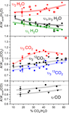 |
Fig. 7 Evolution of the effective IR band strengths, normalised to the corresponding band strength in the pure ice, as a function of the CO2:H2O molecular ratio. Filled symbols indicate results from this work. Squares are for H2O:CO2 binary mixtures, inverted triangles are for H2O:CO2:CO ternary mixtures with 20% CO:H2O, circles are for H2O:CO2:CO ternary mixtures with 40% CO:H2O ratio. The coloured lines indicate the main trends and are drawn only as a guide for the eye. Open squares correspond to CO2:H2O binary mixtures from the literature, which in the upper panel are from Oberg et al. (2007), while in the middle panel they are from Gerakines et al. (1995) |
4 Summary and conclusions
In this work, visible refractive indices (for λ = 632.8 nm), mass densities, mid-IR optical constants, and band strengths have been determined for single species ices of H2O, CO2, and CO and for binary and ternary ice mixtures of these molecules. The ices were produced by background gas deposition on a substrate held at 10 K and for the range of mixing ratios relevant for ices in dense molecular clouds as revealed by recent observations with JWST. The visible refractive indices, n633, of pure ices and mixtures were obtained from double interferometry measurements during ice growth, and the bulk densities of the H2O, CO2, and CO ices were derived with the Lorentz-Lorenz relation using polarisabilities from the literature. The IR spectra were recorded in the 5000-500 cm−1 range, and the IR complex refractive indices (optical constants), i.e. n(ν), k(ν), for the single species ices and ice mixtures were obtained using the freely available software of Gerakines & Hudson (2020). The main conclusions of this study are summarised as follows:
As expected, low density (porous) ices formed in our experiments. Our measured visible refractive indices (632.8 nm) and densities for pure H2O, CO2, and CO ices are in good agreement with previous literature values for background deposited ices.
The densities of the mixed ices were estimated using calibrated gas flows and interference measurements. They were found to be higher than the nominal mean values, that is, the values calculated by averaging the densities of the pure ices according to the proportions of each component in the mixture. This suggests that in the simultaneous deposition, CO and CO2 molecules induce structural changes that lead to a compaction of the mixtures.
Inspection of the IR spectra of pure ices shows that under our experimental conditions (T= 10 K, ice growth rate 15 μm/h), H2O ice is amorphous, CO2 is a mixture of amorphous and crystalline ice, and CO is crystalline (α CO). In the binary and ternary mixtures, significant changes are observed in the profiles of the main IR absorption bands with respect to those of the single species.
Comparison of our IR optical constants - n(ν), k(ν) - of single species ices with previous literature data showed that the k(ν) is sensitive to the ice morphology. Smaller k(ν) values were obtained for the porous ices in this work compared to the more compact ices from directional deposition reported in the literature. The libration band of pure H2O ice seems to be sensitive to the structure and not just to the associated lower density, but more work is needed to clarify this point.
Significant changes were observed in the IR optical constants n(ν), k(ν), of the ice mixtures. The intensity variations of the k(ν) corresponding to a given absorption band follow the partial molecular density changes of the band carrier in the mixture, but k(ν) is also affected by variations in the morphology or by the chemical environment, and disentangling these complex factors is not easy. On the other hand, as previously mentioned, compaction is observed in the co-deposited mixtures. This suggests that morphological differences between directionally and background-deposited mixed ices may be smaller than those observed in single-species ices.
The band strength, which is a molecular property, is not expected to be too sensitive to the ice morphology, but a proper molecular density must be used for its derivation. We find that a careful consideration of the likely ice morphology (density) in different experiments could clarify discrepancies in the published data on single species ices.
Band strengths change in the mixed ices with respect to the single species. The largest variations observed over the range of mixing ratios studied here are on the order of 20%. Changes upon mixing depend on the specific vibrational mode. The band strengths of stretching vibrations are smaller in the mixtures than in the pure ices. In contrast, bending vibrations often have larger band strengths in the mixed ices.
The results of this work extend the studies on optical constants for ice mixtures to ices involving the three major species constitutive of grain mantles. They provide the lacking data for a range of relevant mixing ratios, and are thus expected to be useful for the interpretation of ice observations with JWST.
Data Availability
The complex IR refractive indices for all the ices studied in this work can be found in the Zenodo repository: https://doi.org/10.5281/zenodo.17223398.
Acknowledgements
BM, RP, JO, IT, and VJH acknowledge support provided by grant no. PID2023-146415NB-I00 funded by MICIU/AEI/10.13039/501100011033. ED and JN acknowledge support from the Thematic Action “Physique et Chimie du Milieu Interstellaire” (PCMI) of INSU Programme National “Astro”, with contributions from CNRS Physique & CNRS Chimie, CEA, and CNES.
References
- Accolla, M., Congiu, E., Dulieu, F., et al. 2011, PCCP, 13, 8037 [Google Scholar]
- Aikawa, Y., Kamuro, D., Sakon, I., et al. 2012, A&A, 538, A57 [NASA ADS] [CrossRef] [EDP Sciences] [Google Scholar]
- Baratta, G. A., & Palumbo, M. E. 1998, J. Opt. Soc. Am. A, 15, 3076 [Google Scholar]
- Baratta, G. A., & Palumbo, M. E. 2017, A&A, 608, A81 [NASA ADS] [CrossRef] [EDP Sciences] [Google Scholar]
- Bergin, E. A., Melnick, G. J., Gerakines, P. A., Neufeld, D. A., & Whittet, D. C. B. 2005, ApJ, 627, L33 [NASA ADS] [CrossRef] [Google Scholar]
- Bernstein, M. P., Cruikshank, D. P., & Sandford, S. A. 2005, Icarus, 179, 527 [NASA ADS] [CrossRef] [Google Scholar]
- Boogert, A. A., Gerakines, P. A., & Whittet, D. C. 2015, Annu. Rev. Astron. Astrophys., 53, 541 [CrossRef] [Google Scholar]
- Bossa, J.-B., Isokoski, K., Paardekooper, D. M., et al. 2014, A&A, 561, A136 [NASA ADS] [CrossRef] [EDP Sciences] [Google Scholar]
- Bossa, J.-B., Maté, B., Fransen, C., et al. 2015, ApJ, 814, 47 [NASA ADS] [CrossRef] [Google Scholar]
- Bouilloud, M., Fray, N., Benilan, Y., et al. 2015, MNRAS, 451, 2145 [Google Scholar]
- Brooke, T. Y., Sellgren, K., & Geballe, T. R. 1999, ApJ, 517, 883 [NASA ADS] [CrossRef] [Google Scholar]
- Brown, D. E., & George, S. M. 1996, J. Phys. Chem., 100, 15460 [Google Scholar]
- Buch, V., & Devlin, J. P. 1991, J. Chem. Phys., 94, 4091 [NASA ADS] [CrossRef] [Google Scholar]
- Caselli, P., Walmsley, C. M., Tafalla, M., Dore, L., & Myers, P. C. 1999, ApJ, 523, L165 [Google Scholar]
- Chiar, J. E., Adamson, A. J., Kerr, T. H., & Whittet, D. C. B. 1995, ApJ, 455, 234 [NASA ADS] [CrossRef] [Google Scholar]
- Clément, A., Taillard, A., Wakelam, V., et al. 2023, A&A, 675, A165 [NASA ADS] [CrossRef] [EDP Sciences] [Google Scholar]
- Dartois, E. 2005, Space Sci. Rev., 119, 293 [NASA ADS] [CrossRef] [Google Scholar]
- Dartois, E., Demyk, K., d’Hendecourt L., & Ehrenfreund, P. 1999, A&A, 351, 1066 [Google Scholar]
- Dartois, E., Ding, J. J., de Barros, A. L., et al. 2013, A&A, 557, A97 [NASA ADS] [CrossRef] [EDP Sciences] [Google Scholar]
- Dartois, E., Noble, J. A., Ysard, N., Demyk, K., & Chabot, M. 2022, A&A, 666, A153 [NASA ADS] [CrossRef] [EDP Sciences] [Google Scholar]
- Dartois, E., Noble, J. A., Caselli, P., et al. 2024, Nat. Astron., 8, 359 [NASA ADS] [CrossRef] [Google Scholar]
- Devlin, J. P., Sadlej, J., & Buch, V. 2001, J. Phys. Chem. A, 105, 974 [Google Scholar]
- Dohnálek, Z., Kimmel, G., Ayotte, P., Smith, R., & Kay, B. 2003, J. Chem. Phys., 118, 364 [CrossRef] [Google Scholar]
- Domingo, M., Luna, R., Satorre, M. A., Santonja, C., & Millan, C. 2015, J. Low Temp. Phys., 181, 1 [Google Scholar]
- Domingo, M., Luna, R., Satorre, M. A., Santonja, C., & Millán, C. 2021, ApJ, 906, 81 [NASA ADS] [CrossRef] [Google Scholar]
- Ehrenfreund, P., Boogert, A., Gerakines, P., Tielens, A., & van Dishoeck, E. 1997, A&A, 328, 649 [NASA ADS] [Google Scholar]
- Elsila, J., Allamandola, L., & Sandford, S. 1997, ApJ, 479, 818 [NASA ADS] [CrossRef] [Google Scholar]
- Escribano, R. M., Munoz Caro, G. M., Cruz-Diaz, G. A., Rodriguez-Lazcano, Y., & Mate, B. 2013, PNAS, 110, 12899 [Google Scholar]
- Furuya, K., Aikawa, Y., Hincelin, U., et al. 2015, A&A, 584, A124 [NASA ADS] [CrossRef] [EDP Sciences] [Google Scholar]
- Garrod, R. T., & Pauly, T. 2011, ApJ, 735, 15 [Google Scholar]
- Gerakines, P. A., & Hudson, R. L. 2015, ApJ, 808 [Google Scholar]
- Gerakines, P. A., & Hudson, R. L. 2020, ApJ, 901 [Google Scholar]
- Gerakines, P., Schutte, W., Greenberg, J., & van Dishoeck, E. 1995, A&A, 296, 810 [NASA ADS] [Google Scholar]
- Gerakines, P., Whittet, D., Ehrenfreund, P., et al. 1999, ApJ, 522, 357 [NASA ADS] [CrossRef] [Google Scholar]
- Gerakines, P. A., Materese, C. K., & Hudson, R. L. 2023, MNRAS, 522, 3145 [NASA ADS] [CrossRef] [Google Scholar]
- Gibb, E., Whittet, D., Boogert, A., & Tielens, A. 2004, ApJSS, 151, 35 [NASA ADS] [CrossRef] [Google Scholar]
- Gonzalez Diaz, C., Carrascosa, H., Munoz Caro, G. M., Satorre, M. A., & Chen, Y.-J. 2022, MNRAS, 517, 5744 [CrossRef] [Google Scholar]
- Hagen, W., Tielens, A., & Greenberg, J. 1981, Chem. Phys., 56, 367 [NASA ADS] [CrossRef] [Google Scholar]
- Hasegawa, T., Yanagisawa, H., Nagasawa, T., et al. 2024, ApJ, 969 [Google Scholar]
- He, J., Emtiaz, S. M., Boogert, A., & Vidali, G. 2018, ApJ, 869 [Google Scholar]
- Herczku, P., Mifsud, D. V., Ioppolo, S., et al. 2021, Rev. Sci. Instrum., 92, 084051 [Google Scholar]
- Hohm, U. 2013, J. Mol. Struct., 1054, 282 [Google Scholar]
- Hudgins, D., Sandford, S., Allamandola, L., & Tielens, A. 1993, ApJSS, 86, 713 [Google Scholar]
- Ioppolo, S., Cuppen, H. M., Romanzin, C., van Dishoeck, E. F., & Linnartz, H. 2008, ApJ, 686, 1474 [NASA ADS] [CrossRef] [Google Scholar]
- Ioppolo, S., van Boheemen, Y., Cuppen, H. M., van Dishoeck, E. F., & Linnartz, H. 2011, MNRAS, 413, 2281 [NASA ADS] [CrossRef] [Google Scholar]
- Isokoski, K., Bossa, J. B., Triemstra, T., & Linnartz, H. 2014, PCCP, 16, 3456 [NASA ADS] [CrossRef] [Google Scholar]
- Jiang, G., Person, W., & Brown, K. 1975, J. Chem. Phys., 62, 1201 [NASA ADS] [CrossRef] [Google Scholar]
- Jorgensen, J., Schöier, F., & van Dishoeck, E. 2005, A&A, 435, 177 [NASA ADS] [CrossRef] [EDP Sciences] [Google Scholar]
- Klotz, A., Ward, T., & Dartois, E. 2004, A&A, 416, 801 [NASA ADS] [CrossRef] [EDP Sciences] [Google Scholar]
- Knez, C., Boogert, A., Pontoppidan, K., et al. 2005, ApJ, 635, L145 [NASA ADS] [CrossRef] [Google Scholar]
- Kouchi, A. 1990, J. Cryst. Growth, 99, 1220 [Google Scholar]
- Kouchi, A., Tsuge, M., Hama, T., et al. 2021a, MNRAS, 505, 1530 [CrossRef] [Google Scholar]
- Kouchi, A., Tsuge, M., Hama, T., et al. 2021b, ApJ, 918, 45 [NASA ADS] [CrossRef] [Google Scholar]
- Lacy, J., Baas, F., Allamandola, L., et al. 1984, ApJ, 276, 533 [NASA ADS] [CrossRef] [Google Scholar]
- Li, H. H. 1976, J. Phys. Chem. Ref. Data, 5, 329 [Google Scholar]
- Loeffler, M. J., Moore, M. H., & Gerakines, P. A. 2016, ApJ, 827, 98 [Google Scholar]
- Luna, R., Millan, C., Domingo, M., Santonja, C., & Satorre, M. A. 2022, ApJ, 935, 134 [NASA ADS] [CrossRef] [Google Scholar]
- Mastrapa, R. M., Sandford, S. A., Roush, T. L., Cruikshank, D. P., & Ore, C. M. D. 2009, ApJ, 701, 1347 [NASA ADS] [CrossRef] [Google Scholar]
- Maté, B., Medialdea, A., Moreno, M., Escribano, R., & Herrero, V. 2003, J. Phys. Chem. B, 107, 11098 [Google Scholar]
- McClure, M. K., Rocha, W. R. M., Pontoppidan, K. M., et al. 2023, Nat. Astron., 7, 431 [NASA ADS] [CrossRef] [Google Scholar]
- Mejia, C., de Barros, A. L. F., Duarte, E. S., et al. 2015, Icarus, 250, 222 [CrossRef] [Google Scholar]
- Narten, A. 1976, J. Chem. Phys., 64, 1106 [NASA ADS] [CrossRef] [Google Scholar]
- Noble, J. A., Dulieu, F., Congiu, E., & Fraser, H. J. 2011, ApJ, 735, 121 [NASA ADS] [CrossRef] [Google Scholar]
- Noble, J. A., Fraser, H. J., Aikawa, Y., Pontoppidan, K. M., & Sakon, I. 2013, ApJ, 775, 85 [Google Scholar]
- Noble, J. A., Fraser, H. J., Smith, Z. L., et al. 2024, Nat. Astron., 8, 1169 [NASA ADS] [CrossRef] [Google Scholar]
- Oba, Y., Miyauchi, N., Hidaka, H., et al. 2009, ApJ, 701, 464 [NASA ADS] [CrossRef] [Google Scholar]
- Oba, Y., Watanabe, N., Kouchi, A., Hama, T., & Pirronello, V. 2010, ApJ, 712, L174 [NASA ADS] [CrossRef] [Google Scholar]
- Oberg, K. I., Fraser, H. J., Boogert, A. C. A., et al. 2007, A&A, 462, 1187 [NASA ADS] [CrossRef] [EDP Sciences] [Google Scholar]
- Oberg, K. I., Boogert, A. C. A., Pontoppidan, K. M., et al. 2011, ApJ, 740, 109 [Google Scholar]
- Palumbo, M. E. 2006, A&A, 453, 903 [NASA ADS] [CrossRef] [EDP Sciences] [Google Scholar]
- Palumbo, M., Baratta, G., Collings, M., & McCoustra, M. 2006, PCCP, 8, 279 [Google Scholar]
- Palumbo, M. E., Baratta, G. A., Leto, G., & Strazzulla, G. 2010, J. Mol. Struct., 972, 64 [NASA ADS] [CrossRef] [Google Scholar]
- Pontoppidan, K. M. 2006, A&A, 453, L47 [NASA ADS] [CrossRef] [EDP Sciences] [Google Scholar]
- Pontoppidan, K., Fraser, H., Dartois, E., et al. 2003, A&A, 408, 981 [NASA ADS] [CrossRef] [EDP Sciences] [Google Scholar]
- Pontoppidan, K. M., Boogert, A. C. A., Fraser, H. J., et al. 2008, ApJ, 678, 1005 [NASA ADS] [CrossRef] [Google Scholar]
- Raut, U., Teolis, B. D., Loeffler, M. J., et al. 2007, J. Chem. Phys., 126, 244511 [NASA ADS] [CrossRef] [Google Scholar]
- Rocha, W. R. M., Rachid, M. G., Olsthoorn, B., et al. 2022, A&A, 668, A63 [NASA ADS] [CrossRef] [EDP Sciences] [Google Scholar]
- Rocha, W. R. M., van Dishoeck, E. F., Ressler, M. E., et al. 2024, A&A, 683, A124 [NASA ADS] [CrossRef] [EDP Sciences] [Google Scholar]
- Ron, A., & Schnepp, O. 1967, J. Chem. Phys., 46, 3991 [NASA ADS] [CrossRef] [Google Scholar]
- Roux, J., Wood, B., Smith, A. M., & Pyler, R. R. 1980, Arnold Engineering Development Center Int. Rep. Final Rep. AEDC-TR-79, Arnold Air Force Station [Google Scholar]
- Rowland, B., Fisher, M., & Devlin, J. 1991, J. Chem. Phys., 95, 1378 [Google Scholar]
- Ruffle, D., & Herbst, E. 2000, MNRAS, 319, 837 [Google Scholar]
- Sandford, S., & Allamandola, L. 1990, ApJ, 355, 357 [NASA ADS] [CrossRef] [Google Scholar]
- Sandford, S., Allamandola, L., Tielens, A., & Valero, G. 1988, ApJ, 329, 498 [NASA ADS] [CrossRef] [Google Scholar]
- Satorre, M. A., Domingo, M., Millan, C., et al. 2008, Planet. Space Sci., 56, 1748 [NASA ADS] [CrossRef] [Google Scholar]
- Schulze, W., & Abe, H. 1980, Chem. Phys., 52, 381 [Google Scholar]
- Shimonishi, T., Onaka, T., Kato, D., et al. 2010, A&A, 514, A12 [NASA ADS] [CrossRef] [EDP Sciences] [Google Scholar]
- Smith, Z. L., Dickinson, H. J., Fraser, H. J., et al. 2025, Nat. Astron., 9, 883 [Google Scholar]
- Sturm, J. A., McClure, M. K., Beck, T. L., et al. 2023, A&A, 679, A138 [NASA ADS] [CrossRef] [EDP Sciences] [Google Scholar]
- Tempelmeyer, K., & Mills. 1968, J. Appl. Phys., 39, 2968 [NASA ADS] [CrossRef] [Google Scholar]
- Tielens, A., Tokunaga, A., Geballe, T., & Baas, F. 1991, ApJ, 381, 181 [NASA ADS] [CrossRef] [Google Scholar]
- van Dishoeck, E. 2004, Annu. Rev. Astron. Astrophys., 42, 119 [Google Scholar]
- Westley, M., Baratta, G., & Baragiola, R. 1998, J. Chem. Phys., 108, 3321 [NASA ADS] [CrossRef] [Google Scholar]
- Willner, S., Gillett, F., Herter, T., et al. 1982, ApJ, 253, 174 [Google Scholar]
- Wood, B., & Roux, J. 1982, J. Opt. Soc. Am., 72, 720 [Google Scholar]
- Yamada, H., & Person, W. 1964, J. Chem. Phys., 41, 2478 [NASA ADS] [CrossRef] [Google Scholar]
- Yang, Y.-L., Green, J. D., Pontoppidan, K. M., et al. 2022, ApJ, 941, L13 [NASA ADS] [CrossRef] [Google Scholar]
NASA optical constats databas: https://ocdb.smce.nasa.gov/; Leiden-Ice-Database for astrochemistry (LIDA): https://icedb.strw.leidenuniv.nl/
All Tables
Measured visible refractive indices, n633, and estimated densities, ρ, of the ices of H2O, CO2, and CO.
Molecular mixing ratios; refractive indices at λ = 632.8 nm; n633 densities, p; and estimated nominal mean densities, ρmn (see the text).
All Figures
|
Fig. 1 a) Scheme of the experimental setup. b) Laser interference signal recorded at two incidence angles, α = 1.3 deg and β = 76. 5 deg, during H2O:CO2:CO 100:26:40 ice growth at 10 K at a constant deposition rate of 4 μm/h. |
| In the text | |
|
Fig. 2 Refractive indices (at λ = 632.8 nm) and densities of H2O:CO2 and H2O:CO2:CO ice mixtures grown by background vapour deposition at 10 K. Lines are drawn to guide the eye. |
| In the text | |
|
Fig. 3 Main mid-IR absorptions in pure ices and in binary and ternary mixtures: (a) OH stretching modes (ν1,ν3) of H2O; (b) antisymmetric stretching mode (ν3) of CO2; (c) stretching mode (ν) of CO; (d) bending (ν2) and libration (ν1) modes of H2O near 1650 and 750 cm−1, respectively, and bending mode (ν2) of CO2 near 657 cm−1 ; (e) enlargement of the ν2 mode of CO2. All bands of a given species presented in a panel correspond to the same number of molecules of that species. Specifically, in panels (a) and (d), NH2O = 4.8 × 10¹⁷ molecules cm−2; in panels (b) and (e) NCO2=1.7 × 10¹⁷ molecules cm−2 ; and in panel (c) NCO = 4.0 × 10¹⁷ molecules cm−2. |
| In the text | |
|
Fig. 4 Imaginary part, k(ν), of the refractive index (optical constant) of H2O (upper panel), CO2 (middle panel), and CO (lower panel) ices and comparison with literature values. The literature sources were the NASA and LIDA optical constants databases, a) Hudgins et al. (1993) b) Mastrapa et al. (2009), c) Rocha et al. (2022), d) Ehrenfreund et al. (1997), e) Baratta & Palumbo (1998), f) Gerakines & Hudson (2020), g) Elsila et al. (1997), h) Palumbo et al. (2006), i) Gerakines et al. (2023). |
| In the text | |
|
Fig. 5 Complex refractive indices of H2O:CO2 ice mixtures grown at 10 K. Solid lines, this work. Dashed line, LIDA database; a) Ehrenfreund et al. (1997). |
| In the text | |
|
Fig. 6 Complex refractive index of H2O:CO2:CO ice mixtures grown at 10 K. The left inset in the upper panel corresponds to the ν3 mode of CO2 (2343 cm−1) and the right inset to the CO stretching mode (2140 cm−1). |
| In the text | |
|
Fig. 7 Evolution of the effective IR band strengths, normalised to the corresponding band strength in the pure ice, as a function of the CO2:H2O molecular ratio. Filled symbols indicate results from this work. Squares are for H2O:CO2 binary mixtures, inverted triangles are for H2O:CO2:CO ternary mixtures with 20% CO:H2O, circles are for H2O:CO2:CO ternary mixtures with 40% CO:H2O ratio. The coloured lines indicate the main trends and are drawn only as a guide for the eye. Open squares correspond to CO2:H2O binary mixtures from the literature, which in the upper panel are from Oberg et al. (2007), while in the middle panel they are from Gerakines et al. (1995) |
| In the text | |
Current usage metrics show cumulative count of Article Views (full-text article views including HTML views, PDF and ePub downloads, according to the available data) and Abstracts Views on Vision4Press platform.
Data correspond to usage on the plateform after 2015. The current usage metrics is available 48-96 hours after online publication and is updated daily on week days.
Initial download of the metrics may take a while.