| Issue |
A&A
Volume 704, December 2025
|
|
|---|---|---|
| Article Number | L13 | |
| Number of page(s) | 9 | |
| Section | Letters to the Editor | |
| DOI | https://doi.org/10.1051/0004-6361/202556850 | |
| Published online | 12 December 2025 | |
Letter to the Editor
Asteroseismic detection of an internal magnetic field in the B0.5V pulsator HD 192575
1
Institute of Astronomy, KU Leuven, Celestijnenlaan 200D, 3001 Leuven, Belgium
2
Department of Astrophysics, IMAPP, Radboud University Nijmegen, PO Box 9010 6500 GL Nijmegen, The Netherlands
3
Max Planck Institute for Astronomy, Königstuhl 17, 69117 Heidelberg, Germany
★ Corresponding author: This email address is being protected from spambots. You need JavaScript enabled to view it.
Received:
13
August
2025
Accepted:
22
November
2025
Abstract
Context. Internal magnetic fields are an elusive component of stellar structure. However, they can play an important role in stellar structure and evolution models through efficient angular momentum transport and through their impact on internal mixing.
Aims. We strive to explain the nine components of one frequency multiplet identified as a low-order quadrupole gravity mode detected in the light curve of the β Cep pulsator HD 192575 assembled by the Transiting Exoplanet Survey Satellite (TESS).
Methods. We updated the frequencies of the quadrupole mode under investigation using a standard pre-whitening method applied to the 1951.46 d TESS light curve. This showed that an internal magnetic field is required to simultaneously explain all nine components. We implemented theoretical pulsation computations applicable to the low-order modes of a β Cep pulsator including the Coriolis force as well as a magnetic field that is misaligned with respect to the rotation axis. We applied the theoretical description to perform asteroseismic modelling of the amplitudes and frequencies in the multiplet of the quadrupole g-mode of this evolved β Cep star.
Results. Pulsation predictions based on the measured internal rotation frequency of the star cannot explain the observed nine-component frequency splittings of the quadrupole low-order gravity mode. By contrast, we show that the combined effect of the Coriolis force caused by the near-core rotation with a period of ∼5.3 d and the Lorentz force due to an internal inclined magnetic field with a maximum strength of ∼24 kG does provide a proper explanation of the nine multiplet frequencies and their relative amplitudes.
Conclusions. Given HD 192575’s stellar mass of about 12 M⊙, this work presents the detection and magneto-gravito-asteroseismic modelling of a stable internal magnetic field buried inside an evolved rotating supernova progenitor.
Key words: asteroseismology / stars: evolution / stars: interiors / stars: magnetic field / stars: oscillations / stars: rotation
© The Authors 2025
 Open Access article, published by EDP Sciences, under the terms of the Creative Commons Attribution License (https://creativecommons.org/licenses/by/4.0), which permits unrestricted use, distribution, and reproduction in any medium, provided the original work is properly cited.
This article is published in open access under the Subscribe to Open model. This email address is being protected from spambots. You need JavaScript enabled to view it. to support open access publication.
1. Introduction
Measured internal rotation rates of intermediate-mass stars are lower than expected based on standard stellar evolution theories. This has led to a debate about the theory of angular momentum transport (Aerts et al. 2019; Aerts & Tkachenko 2024). Moreover, near-uniform rotation has been reported for main-sequence stars with masses between 1.3 M⊙ and 3.3 M⊙ (Aerts 2021), and low levels of differential rotation between one and two are reported to occur for the β Cep pulsators (8 M⊙ ≤ M ≤ 25 M⊙, Fritzewski et al. 2025). These asteroseismic results indicate an angular momentum transport problem, where the transport occurs more efficiently than predicted early on in the lives of stars.
Along with internal gravity waves, internal magnetic fields are expected to efficiently transport angular momentum. Such fields could possibly also explain the near-uniform rotation rates of stars in core-hydrogen or core-helium burning stages (Aerts et al. 2019). While surface magnetic fields have been widely detected for most types of stars (Landstreet 1992; Donati & Landstreet 2009), internal fields are notoriously difficult to detect and characterise. The internal magnetic fields in the radiative envelope of intermediate- and high-mass stars are thought to be of fossil origin (Mestel 1999; Neiner et al. 2015), where the field is a remnant of a primordial magnetic field present during the star formation process.
Asteroseismology provides a unique and promising opportunity to study internal magnetic fields buried beneath the surface by probing stellar interiors through non-radial oscillations. This has been achieved from ground-based asteroseismology for the strongly magnetic, rapidly oscillating Ap (roAp) stars (Kurtz 1982) and has led to the oblique pulsator model (Shibahashi & Takata 1993; Bigot & Dziembowski 2002). This model was successfully applied to explain the multiplet behaviour of the dominant radial mode in the prototypical star β Cephei (Shibahashi & Aerts 2000). Since the space asteroseismology era, internal magnetic fields have been detected in red giants (Li et al. 2022, 2023; Deheuvels et al. 2023; Hatt et al. 2024) and interpreted by the theoretical frameworks developed by Gomes & Lopes (2020), Mathis et al. (2021), Loi (2021), Li et al. (2022), Bugnet (2022), and Mathis & Bugnet (2023). Aside from direct magnetically induced frequency detections in roAp stars and β Cephei, the presence of internal magnetic fields in intermediate- or high-mass main-sequence stars is indirect and based on theory (Aerts et al. 2021; Rui et al. 2024), numerical simulations (Lecoanet et al. 2022), or inferences from depressed dipole modes in red giants (Fuller et al. 2015; Stello et al. 2016). In this letter, we report the direct detection as well as asteroseismic modelling of an internal magnetic field in a ∼12 M⊙ evolved main-sequence star from one of its low-order pulsation modes, which occurs far outside the asymptotic regimes of low or high frequencies (see Fig. 3 in Aerts & Tkachenko 2024).
2. Observational input and equilibrium models
The early-type B0.5V star HD 192575 was discovered to be a β Cep pulsator by Burssens et al. (2023). They analysed its 324 d light curve obtained in Cycle 2 of the Transiting Exoplanet Survey Satellite (TESS; Ricker et al. 2015) and deduced a rich oscillation spectrum with several multiplets of low-order, low-degree pressure and gravity modes. The authors additionally derived an effective temperature of Teff = 23 900 ± 900 K, a surface gravity of log g = 3.65 ± 0.15, and the rotation velocity projected onto the line of sight,  km/s, from spectra.
From stellar evolution models computed with the MESA software (Modules for Experiments in Stellar Astrophysics, Version 12778, Paxton et al. 2019) HD 192575 was found to have a mass between 11 and 13 M⊙. The star is in an evolved stage approaching the end of the main sequence, as X ≤ 0.25 in its convective core. This was derived from forward seismic modelling by Vanlaer et al. (2025), who used the Cycles 2, 4, and 5 TESS light curves. From rotation inversions, this study also led to a well-constrained rotation frequency of about 0.2 d−1 in the near-core region and a ratio of the core-to-surface rotation between 0.4 and 1.8. This is in agreement with the result of 1.4 obtained from 2D evolution models (Mombarg et al. 2024).
Following TESS Cycles 2, 4, 5, and 6, HD 192575 has a 2-minute cadence light curve covering 1951.46 d (Rayleigh frequency resolution of ∼5 × 10⁻⁴ d−1) with a duty cycle of 43%. Figure A.1 shows its Lomb-Scargle periodogram. We performed a new frequency analysis to extract the periodic signal in this light curve as an improvement to the results in Burssens et al. (2023) and Vanlaer et al. (2025) owing to the addition of the data of Cycle 6 (up to December 2024). We applied classical pre-whitening, extracting the dominant frequency at each step; optimising its value, amplitude, and phase from non-linear regression; and computing a residual curve for the next iteration. This was done with an adapted version of the STAR SHADOW software (IJspeert et al. 2024). All the extracted frequencies with a local signal-to-noise ratio (S/N) above two are provided electronically through CDS, where the S/N is calculated as the ratio of the extracted amplitude to the mean amplitude in a window of 1 d−1 centered on the frequency of interest. Each frequency in the nine-component multiplet is given an identifier, fgj, where the index j increases from low to high frequencies. All considered frequencies have at least S/N > 9. The new data led to the additional detection of fg2 compared to Vanlaer et al. (2025) and fg2 and fg9 compared to Burssens et al. (2023).
For the purpose of this letter, we relied on the forward models that fit the 15 identified frequencies within the four multiplets selected and identified by Vanlaer et al. (2025). We focus on the multiplet of the quadrupole gravity (g-)mode at 3.8 d−1, as it is the only multiplet in the entire oscillation spectrum revealing more frequencies than can be explained by rotational splitting of a single mode. Based on the seven available frequencies from Cycle 2, Burssens et al. (2023) interpreted the selected g-mode multiplet as resulting from two merged quadrupole modes undergoing an avoided crossing (Aizenman et al. 1977). However, the more extended light curve used by Vanlaer et al. (2025) revealed that the avoided crossing assumption is invalid unless the spectroscopic error box is enlarged to 3σ in Teff and log g. Because of this, Vanlaer et al. (2025) selected additional model sets fitting the 15 identified frequencies, among which are the quadrupole low-order g-modes with the five frequencies fg1, fg4, fg6, fg7, and fg9. The authors assumed these frequencies form a complete rotationally split asymmetric quintuplet, leaving the other frequencies in Fig. A.2 unexplained. The additional detected oscillation frequency in our analysis, fg2, decreased the maximum spacing between the two adjacent modes in the avoided crossing from 0.18 d−1 to 0.02 d−1. None of the stellar models in the model grid of Burssens et al. (2023) used by Vanlaer et al. (2025) allow for such a constraint, irrespective of any spectroscopic cut, thus firmly excluding the interpretation of an avoided crossing. The new data thus leave only an internal magnetic field as the unexplored avenue to interpret all nine observed frequencies simultaneously, as spectroscopy revealed the star to be single. Hence, we included the effect of a magnetic field in a theoretical pulsation model, which is capable of explaining all nine frequencies in Fig. A.2 from models within the 1σ spectroscopic box of the star fitting the 15 selected and identified multiplet frequencies considered by Vanlaer et al. (2025).
3. Theoretical pulsation approximation
We calculated the effects of rotation and an internal magnetic field on the oscillation modes of the star. To do so, we considered these effects in a first-order approximation ignoring the centrifugal force. This is justified given the modest rotation rate and the mode under study having a spin parameter of ∼10%. Moreover, the quadrupole g-mode’s rotation kernel is dominant near the convective core for most models. We assumed solid body rotation as a proxy for the average rotation rate in the region where the g-mode probes. Under these circumstances we could rely on the theoretical framework of Loi (2021) for red giants to calculate the relative amplitudes and frequencies of the oscillation modes. We did so for the six model sets in Vanlaer et al. (2025), whose properties are repeated in Table A.1.
The eigenfrequency, ω0, for the corresponding eigenvector, ξ, of an oscillation mode in the absence of rotation and internal magnetic fields follows from the equation (Gough & Thompson 1990; Aerts et al. 2010)
 (1)
(1)
describing the mode as a consequence of linear perturbations in the density, ρ; pressure, p; and the gravitational acceleration, g. Following Loi (2021), we included the effects of rotation and a misaligned internal magnetic field by perturbing Eq. (1):
 (2)
(2)
where δℱrot and δℱmag describe the effects of rotation and an internal magnetic field, respectively. These effects lead to a change, δω, in the eigenfrequency. By describing these additional effects perturbatively, we assumed their influence to be small compared to ℱ0. The description and formulation of the first-order perturbative approach is given in Appendix B and follows the work of Loi (2021). This approach leads to the equation describing the effect of rotation and an internal magnetic field as
 (3)
(3)
When the rotation axis and magnetic field axis are aligned, the Wigner d-matrix, D, is the unit matrix, and we obtained 2l + 1 frequencies. If the axes are misaligned, the matrix  is non-diagonal and generally leads to (2l + 1)2 frequencies. Each independent solution consisting of 2l + 1 frequencies describes a single mode of the star. For this to hold, the relative amplitudes must be fixed and can be calculated using Eq. (3), where they are the elements of the eigenvector r. We refer to Loi (2021) and Vandersnickt (2025) for an in-depth description and discussion of the mathematical magneto-rotational pulsation model.
To include the amplitudes in the fitting of the modes, we considered the inclination angle, i, between the rotational axis and the line of sight, and we only considered the geometric effects (Gizon & Solanki 2003). For brightness variations, I, on the stellar surface following
 (4)
(4)
the amplitude correction factor is  , which is given by (Dziembowski 1977; Toutain & Gouttebroze 1993)
![Mathematical equation: $$ \begin{aligned} \mathcal{E} (i) = \frac{(l - |m|)!}{(l + |m|)!} \left[ P^{|m|}_l ( \sin i)\right]^2. \end{aligned} $$](/articles/aa/full_html/2025/12/aa56850-25/aa56850-25-eq8.gif) (5)
(5)
This framework allows for the simultaneous fitting of frequency and amplitude. Throughout this work, we use a reference frame with a polar axis equal to the rotation axis of the star.
We considered a fossil magnetic field topology as described in Duez & Mathis (2010), where we parametrised the field by its maximum magnetic field strength, Bmax, and used the solutions with the largest radial scales. By assuming a fixed topology, we reduced the number of free parameters considerably. We minimised the impact of the chosen topology on the results by modelling the modes independently, as different modes have different sensitivity kernels in the stellar interior. The magnetic field was constrained to the radiative envelope of the star in a dipole-like configuration having a poloidal and a toroidal component. As the magnetic field topology is assumed to be axisymmetric along the magnetic axis, we extended the calculation of the elements of Mmag and the corresponding eigenfunctions to two dimensions. In Appendix E we discuss the sensitivity of the modes on the selected magnetic field geometry.
4. New modelling results
Vanlaer et al. (2025, Table 2) revisited the asteroseismic modelling of HD 192575 and determined six sets of acceptable models with different identifications for four multiplets. We relied on these models in all the sets, but for brevity we only report results from the fifth set (Set 5). The full results are available in Vandersnickt (2025) and summarised in Table D.1. Our novel discovery and modelling results do not depend on the chosen set.
For each equilibrium model in the sets, we calculated the eigenfrequencies (ω0) and eigenfunctions (ξ) in absence of rotation and internal magnetic fields using GYRE (Goldstein & Townsend 2020). For each mode, we subsequently calculated the change in frequency and the relative amplitudes using Eq. (B.3). This was done using an iterative process starting from a wide range of magnetic field strengths, rotational frequencies, and obliquity angles and refining as needed.
Extensive testing showed proper convergence, where a modified χ2-type metric, d2, defined as
 (6)
(6)
was used, where the sum included the n observed frequencies and the N ≥ n predicted frequencies among all independent predictions in the multiplet to explain the nine observed frequencies and Δ fi ≡ fi − fcen for a chosen central frequency, fcen, with selected azimuthal order m. We selected fg5 as the central frequency and assumed an azimuthal order of m = 0. This choice is justified as there are frequencies present for each azimuthal order in the rotational splitting, which suggests fg5 and fg6 to have an azimuthal order of m = 0. Correspondingly, we considered only the theoretical frequency differences relative to a predicted frequency with m = 0, drastically decreasing computation time by limiting the azimuthal identification of the different frequencies. The weight, c, is a free parameter to fit the observed amplitudes. The difference in summation between the frequencies and amplitudes is to penalise the fit for predicted signals that are not observed. For the predicted amplitudes with no observed counterpart, we set Ai, obs = 0 μmag and σAi, obs = 1.6 μmag, which is the uncertainty on the extracted amplitudes according to the red noise corrected formulae of Montgomery & O’Donoghue (1999). Using this metric, we calculated the corresponding confidence intervals using the F statistic (see Appendix C).
We applied our fitting process to the split g-mode in Fig. A.2, which was identified to be a g1 (Sets 1 and 2) or g2 mode (Sets 3 to 6) by Vanlaer et al. (2025). In doing so we set the fitting weight parameter to c = 104. This value is necessary to avoid overfitting in frequencies, as the different relative uncertainties between the frequencies and amplitudes would otherwise lead solely to frequency optimisation in the (2l + 1)2 available frequencies. Our new magneto-gravito-asteroseismic modelling can explain all the observed frequencies in the multiplet, as illustrated for a model from Set 5 in Fig. 1. The predicted frequencies show a good agreement with the observed frequencies and amplitudes. As there were only nine observed frequencies and our best pulsation model has a minimum of ten predicted frequencies when two independent (2l + 1) solutions are considered, an explanation of at least one missing frequency was required. The black cross in Fig. 1 shows this unidentified frequency for the best-fitting model. This frequency and its uncertainty is mostly low in amplitude and close to the mean noise level of the periodogram. The best-fitting solution for Set 5 has a maximum magnetic field strength of  kG. While the uncertainty on this value is large, the detection of the internal magnetic field follows from the detection of nine frequencies for the l = 2 multiplet in the updated frequency list. We calculated the sensitivity kernels of the best-fitting mode following Das et al. (2020) and found the sensitivity to peak at Rpeak = 0.994 Rstar, indicating that the mode mostly probes the magnetic field in the near-surface region. The mean magnetic field strength at that radius is Bpeak = 6.85 kG. The large uncertainty on Bmax is connected to the large diversity of magnetic kernel sensitivities for the models in Set 5, with a significant fraction of the models probing the near-core magnetic field. Following Fuller et al. (2015) and Stello et al. (2016), the quadrupole mode can only propagate in the magnetic interior if the magnetic field strength is below the critical value Bcrit, which ranges from ∼107 kG near the core to ∼102 kG near the surface, well above the magnetic field strengths of all accepted models in the 95% confidence interval. This is an additional validation of the perturbative approach, and it reinforces the importance of the Coriolis force and the value of including the centrifugal force in future modelling of the modes.
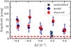 |
Fig. 1. Predictions of the best-fitting magneto-gravito pulsation model from Set 5 and its uncertainties (dark blue). The black cross indicates a predicted frequency not detected in the data. The blue shaded area shows all possible locations of unidentified frequencies. The dashed red line shows the local average noise level in the data. The 95% confidence intervals for the predicted frequency differences are smaller than the size of the markers. |
The obliquity angle, β, and the inclination angle are consistent between the different model sets, with Set 5 giving  and
and  . The inclination angle has no dependence on the radial order of the mode, and it only depends on the azimuthal order, m, of the frequencies and the angular degree, l, of the mode. The value of β is determined by the small splitting and relative amplitudes, while i is sensitive to the relative amplitudes between the frequencies. The rotational frequency estimation of
  d−1 corresponds closely to the results of Vanlaer et al. (2025). We additionally computed the projected rotational velocity v sin i of the star. This includes the uncertainties on the inclination angle, i; the rotational frequency, frot; and the stellar radius. The outcome is consistent with the spectroscopic result of
  km s−1. We find the near-core rotational velocity of the star to be around ∼20% of the Kepler critical velocity, in line with the results of Aerts & Tkachenko (2024). All the best-fitting model parameters are listed in Table D.1 with the 95% confidence intervals per model set. We find that the stellar parameter estimates based on our magnetic description are in agreement with the earlier modelling results by Burssens et al. (2023) and Vanlaer et al. (2025) based on a rotating non-magnetic star.
5. Conclusions
We have presented the asteroseismic detection of an internal magnetic field inside a massive pulsator. We explain the nine observed frequency components of the quadrupole g-mode of the β Cep star HD 192575 as being the combined effects of an internal magnetic field and rotation, where the magnetic and rotation axes are inclined. The detected nine-frequency signature of this l = 2 mode cannot be explained by any currently available pulsation theory for low-order low-degree (l < 3) modes in a single star without invoking an internal magnetic field.
We focused our novel modelling work on the only multiplet detected in the star’s light curve having more than the usual 2l + 1 components induced by internal rotation after excluding the possibility of an avoided crossing between low-order modes. The star also reveals several p-mode multiplets that are well explained by the forward models used here when ignoring the magnetic field. We did not focus on these multiplets to assess the internal magnetic field because the theory we developed is not optimal to model p-modes with rotation kernels peaking in a stellar envelope deformed by the rotation of the star. As shown by Vanlaer et al. (2025), the centrifugal force needs to be included for a proper description of the low-order p-modes of HD 192575. This requires a more complex theoretical description of the rotation based on coupling between modes of different degrees, which is currently under construction. Nevertheless, we already applied our perturbative magnetic pulsation model to the quadrupole p-mode centered at 6.5 d−1 as a sanity check. The results in Appendix D show that such simplified magneto-acoustic modelling is able to explain the four frequencies in this multiplet, with stellar parameters and rotation in agreement with those found above. This good result for the p-mode encourages us to extend the current theoretical pulsation model to include the centrifugal deformation. Such novel theoretical development is underway and will be used to improve the modelling presented here.
Data availability
The full frequency list is available at the CDS via https://cdsarc.cds.unistra.fr/viz-bin/cat/J/A+A/704/L13
Acknowledgments
We thank the referee for valuable comments which helped us to improve our paper. JV, MV, and CA acknowledge funding from the European Research Council (ERC) under the Horizon Europe programme (Synergy Grant agreement N°101071505: 4D-STAR). While funded by the European Union, views and opinions expressed are however those of the author(s) only and do not necessarily reflect those of the European Union or the European Research Council. Neither the European Union nor the granting authority can be held responsible for them. CA also acknowledges support from long term structural funding – Methusalem funding by the Flemish Government (project SOUL, METH/24/012) at KU Leuven. VV and MV additionally acknowledge support from the Research Foundation Flanders (FWO) under grant agreement N°1156923N (PhD Fellowship) and from the KU Leuven Research Council (doctoral mandate grant DB/24/008), respectively. The TESS data presented in this paper were obtained from the Mikulski Archive for Space Telescopes (MAST) at the Space Telescope Science Institute (STScI), which is operated by the Association of Universities for Research in Astronomy, Inc., under NASA contract NAS5-26555. Support to MAST for these data is provided by the NASA Office of Space Science via grant NAG5-7584 and by other grants and contracts. Funding for the TESS mission was provided by the NASA Explorer Program.
References
- Aerts, C. 2021, Rev. Mod. Phys., 93, 015001 [Google Scholar]
- Aerts, C., & Tkachenko, A. 2024, A&A, 692, R1 [NASA ADS] [CrossRef] [EDP Sciences] [Google Scholar]
- Aerts, C., Christensen-Dalsgaard, J., & Kurtz, D. W. 2010, Asteroseismology (Dordrecht: Springer) [Google Scholar]
- Aerts, C., Mathis, S., & Rogers, T. M. 2019, ARA&A, 57, 35 [Google Scholar]
- Aerts, C., Augustson, K., Mathis, S., et al. 2021, A&A, 656, A121 [NASA ADS] [CrossRef] [EDP Sciences] [Google Scholar]
- Aizenman, M., Smeyers, P., & Weigert, A. 1977, A&A, 58, 41 [NASA ADS] [Google Scholar]
- Bigot, L., & Dziembowski, W. A. 2002, A&A, 391, 235 [NASA ADS] [CrossRef] [EDP Sciences] [Google Scholar]
- Bugnet, L. 2022, A&A, 667, A68 [NASA ADS] [CrossRef] [EDP Sciences] [Google Scholar]
- Burssens, S., Bowman, D. M., Michielsen, M., et al. 2023, Nat. Astron., 7, 913 [NASA ADS] [CrossRef] [Google Scholar]
- Das, S. B., Chakraborty, T., Hanasoge, S. M., & Tromp, J. 2020, ApJ, 897, 38 [NASA ADS] [CrossRef] [Google Scholar]
- Deheuvels, S., Li, G., Ballot, J., & Lignières, F. 2023, A&A, 670, L16 [NASA ADS] [CrossRef] [EDP Sciences] [Google Scholar]
- Donati, J. F., & Landstreet, J. D. 2009, ARA&A, 47, 333 [Google Scholar]
- Duez, V., & Mathis, S. 2010, A&A, 517, A58 [NASA ADS] [CrossRef] [EDP Sciences] [Google Scholar]
- Dziembowski, W. 1977, Acta Astron., 27, 203 [NASA ADS] [Google Scholar]
- Fritzewski, D. J., Vanrespaille, M., Aerts, C., et al. 2025, A&A, 698, A253 [NASA ADS] [CrossRef] [EDP Sciences] [Google Scholar]
- Fuller, J., Cantiello, M., Stello, D., Garcia, R. A., & Bildsten, L. 2015, Science, 350, 423 [Google Scholar]
- Gizon, L., & Solanki, S. K. 2003, ApJ, 589, 1009 [Google Scholar]
- Goldstein, J., & Townsend, R. H. D. 2020, ApJ, 899, 116 [NASA ADS] [CrossRef] [Google Scholar]
- Gomes, P., & Lopes, I. 2020, MNRAS, 496, 620 [NASA ADS] [CrossRef] [Google Scholar]
- Gough, D. O., & Thompson, M. J. 1990, MNRAS, 242, 25 [Google Scholar]
- Hatt, E. J., Ong, J. M. J., Nielsen, M. B., et al. 2024, MNRAS, 534, 1060 [NASA ADS] [CrossRef] [Google Scholar]
- IJspeert, L. W., Tkachenko, A., & Johnston, C. 2024, A&A, 685, A62 [NASA ADS] [CrossRef] [EDP Sciences] [Google Scholar]
- Kurtz, D. W. 1982, MNRAS, 200, 807 [NASA ADS] [CrossRef] [Google Scholar]
- Landstreet, J. D. 1992, A&AR, 4, 35 [Google Scholar]
- Lecoanet, D., Bowman, D. M., & Van Reeth, T. 2022, MNRAS, 512, L16 [NASA ADS] [CrossRef] [Google Scholar]
- Li, G., Deheuvels, S., Ballot, J., & Lignières, F. 2022, Nature, 610, 43 [NASA ADS] [CrossRef] [Google Scholar]
- Li, G., Deheuvels, S., Li, T., Ballot, J., & Lignières, F. 2023, A&A, 680, A26 [NASA ADS] [CrossRef] [EDP Sciences] [Google Scholar]
- Loi, S. T. 2021, MNRAS, 504, 3711 [NASA ADS] [CrossRef] [Google Scholar]
- Mathis, S., & Bugnet, L. 2023, A&A, 676, L9 [NASA ADS] [CrossRef] [EDP Sciences] [Google Scholar]
- Mathis, S., Bugnet, L., Prat, V., et al. 2021, A&A, 647, A122 [EDP Sciences] [Google Scholar]
- Mestel, L. 1999, Int. Ser. Monographs. Phys., 99 [Google Scholar]
- Mombarg, J. S. G., Rieutord, M., & Espinosa Lara, F. 2024, A&A, 683, A94 [NASA ADS] [CrossRef] [EDP Sciences] [Google Scholar]
- Montgomery, M. H., & O’Donoghue, D. 1999, Delta Scuti Star Newsletter, 13, 28 [NASA ADS] [Google Scholar]
- Neiner, C., Mathis, S., Alecian, E., et al. 2015, Proc. Int. Astron. Union, 305, 61 [Google Scholar]
- Paxton, B., Smolec, R., Schwab, J., et al. 2019, ApJS, 243, 10 [Google Scholar]
- Ricker, G. R., Winn, J. N., Vanderspek, R., et al. 2015, JATIS, 1, 014003 [Google Scholar]
- Rui, N. Z., Ong, J. M. J., & Mathis, S. 2024, MNRAS, 527, 6346 [Google Scholar]
- Shibahashi, H., & Aerts, C. 2000, ApJ, 531, L143 [NASA ADS] [CrossRef] [Google Scholar]
- Shibahashi, H., & Takata, M. 1993, PASJ, 45, 617 [NASA ADS] [Google Scholar]
- Stello, D., Cantiello, M., Fuller, J., et al. 2016, Nature, 529, 364 [Google Scholar]
- Toutain, T., & Gouttebroze, P. 1993, A&A, 268, 309 [NASA ADS] [Google Scholar]
- Vandersnickt, J. 2025, MSc Thesis, KU Leuven, Belgium [Google Scholar]
- Vanlaer, V., Bowman, D. M., Burssens, S., et al. 2025, A&A, 701, A5 [NASA ADS] [CrossRef] [EDP Sciences] [Google Scholar]
Appendix A: Relevant frequencies of HD 192575
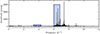 |
Fig. A.1. Lomb-Scargle periodogram of the TESS Cycle 2,4,5, and 6 light curve of HD 192575. The indicated areas are discussed in this Letter. |
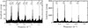 |
Fig. A.2. Excerpt of the Lomb-Scargle periodogram of HD 192575 zoomed in on the g-mode (left) and p-mode (right) multiplet under study. The dotted lines indicate the frequencies extracted from the data and their mode labels. |
Best stellar parameters for the different sets of stellar models used in this work, as determined by Vanlaer et al. (2025).
Appendix B: Perturbative formulation
The perturbation as a consequence of rotation is given by
 (B.1)
(B.1)
where Ω is the rotation vector of the star.
The magnetic perturbation operator for an internal magnetic field B0 is given by
![Mathematical equation: $$ \begin{aligned} \begin{aligned} \delta \mathbf {\mathcal F}_{\mathbf {mag}} \ \boldsymbol{\xi }&= \frac{1}{\rho _0}\left[\mathbf B_0 \times \left[\mathbf \nabla \times \left( - \mathbf B_0 (\mathbf \nabla \cdot \boldsymbol{\xi }) + (\mathbf B_0 \cdot \mathbf \nabla )\boldsymbol{\xi } - (\boldsymbol{\xi } \cdot \mathbf \nabla )\mathbf B_0 \right) \right] \right] \\&+ \frac{1}{\rho _0}\left[(\mathbf \nabla \times (\boldsymbol{\xi } \times \mathbf B_0 ))\times (\mathbf \nabla \times \mathbf B_0 ) \right] - \frac{\rho ^{\prime }}{\rho _0^2}(\mathbf \nabla \times \mathbf B_0 )\times \mathbf B_0 . \end{aligned} \end{aligned} $$](/articles/aa/full_html/2025/12/aa56850-25/aa56850-25-eq40.gif) (B.2)
(B.2)
These first-order approximations require the rotational frequency Ω ≪ ω0 and the Alvén wave frequency ωA ≪ ω0 and additionally ignore any deformation of the star.
We allowed for an obliquity angle β between the rotation axis and the magnetic field axis. The change in the eigenfrequency is consequently given by
 (B.3)
(B.3)
where we have
 (B.4)
(B.4)
 (B.5)
(B.5)
with l the angular degree and m the azimuthal order and where D(β) is the Wigner d-matrix describing the change in frame between the oblique rotation and magnetic field frames, such that each matrix M is calculated in its respective reference frame. ⟨.,.⟩ denotes the inner product of the eigenvectors ξ over the star. Equation (3) is obtained by projecting the magnetic modes to the corotating frame.
Appendix C: Calculating the likelihood function confidence regions
For each combination of parameters, we obtain a distance d2 between the observed and predicted frequencies and amplitudes. The best-fitting model minimises this distance to dmin2. For each model, we can calculate the F statistic to compare with the best fit. This statistic is a measure of the difference in the explained variance expressed by the distance and is given by
 (C.1)
(C.1)
for a number of observables N, and a number of free parameters K. The F statistic is distributed as an F distribution with K and N − K degrees of freedom. This leads to an asymptotic 100(1 − α)% confidence region of the parameters θ, given by
 (C.2)
(C.2)
We take K = 4 to estimate the parameters connected to rotation and the internal magnetic field. The uncertainty intervals in Tables D.1 and D.2 show these parameters of the magnetic field and rotation. The uncertainties on the other parameters can be interpreted as the interval necessary to obtain the corresponding uncertainty in the magnetic field and rotation parameters.
Equation C.1 gives the expected distribution of the F statistic based on the metric d2. We can use this distribution to define a likelihood function for a set of parameters θ, given by
 (C.3)
(C.3)
Appendix D: Results for each model set for both quadrupole modes
The fitting process of the p-mode centered on 6.5 d−1 shown in Figs A.1 and A.2 differs slightly from the one for the g-mode, as we can only consider four observed frequencies in the multiplet. We identified fp3 as the central frequency fcen by comparing the relative amplitudes to the g-mode. We additionally required the predicted set of frequencies to consist of a single independent magnetic solution, as no clear splittings aside from those expected from rotation are available. The weight parameter was set to c = 103.
Figure D.1 shows the best-fitting frequencies and amplitudes for the models in Set 5. There is a good agreement between the observed and predicted frequencies. The best-fitting model predicts an additional frequency that is not identified in the observed frequencies, but it has a low amplitude. The narrow frequency confidence interval on the predicted frequencies can be immediately connected to the low uncertainty on the predicted rotational frequency reported in Table D.2, as this factor has the largest and most direct impact on the predicted frequencies. All predicted parameters are similar to the values derived from the g-mode fittings described in the main text.
Best model parameters and 95% confidence intervals for the asteroseismic modelling of the g-mode.
Best model parameters and 95% confidence intervals for the asteroseismic modelling of the p-mode.
The probing depth of the kernel for the best model in Set 5 peaks at Rpeak = 0.996 Rstar with a magnetic field strength average of Bpeak = 1.86 kG at that radius. The maximum field strength is  kG. The current framework ignores the centrifugal force, the deformation it induces in the stellar envelope, and the accompanying couplings between spheroidal and toroidal components caused by that force. In addition to this omission, the internal magnetic field could also be more complex than a dipole-like field. These effects will be especially important to model p-mode splittings for HD 192575, which has been classified as a moderate rotator by Aerts & Tkachenko (2024).
The predicted projected rotational velocity v sin i is again consistent with the previous estimate by Burssens et al. (2023), with a larger uncertainty due to the larger uncertainty on the inclination angle i.
Appendix E: Kernel sensitivity
Following the results of Das et al. (2020), the sensitivity of the modes to the internal magnetic field can be decomposed as a product of the magnetic stress tensor BB and the sensitivity kernel K as
 (E.1)
(E.1)
where ":" denotes the tensor product. Figure E.1 shows an example of the magnetic sensitivity kernel. The sensitivity peak is near the surface for this example and varies by multiple orders of magnitudes throughout the interior. Other cases are possible where the sensitivity is strongly peaked near the core, leading to higher magnetic field strengths required for a similar effect on the modes.
Figure E.2 shows the magnetic stress tensor for an example magnetic field topology used. These figures show that the maximum magnetic field value is not at the edges of the field. The magnetic field strength peak is, however, deep in the envelope close to the core.
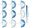 |
Fig. E.1. Magnetic sensitivity kernel of an example g mode with n = −1, l = 2. Magnetic sensitivity kernel of an example g mode with n = −1, l = 2. |
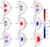 |
Fig. E.2. Magnetic stress tensor of an example magnetic field used following the prescription of Duez & Mathis (2010). |
All Tables
Best stellar parameters for the different sets of stellar models used in this work, as determined by Vanlaer et al. (2025).
Best model parameters and 95% confidence intervals for the asteroseismic modelling of the g-mode.
Best model parameters and 95% confidence intervals for the asteroseismic modelling of the p-mode.
All Figures
|
Fig. 1. Predictions of the best-fitting magneto-gravito pulsation model from Set 5 and its uncertainties (dark blue). The black cross indicates a predicted frequency not detected in the data. The blue shaded area shows all possible locations of unidentified frequencies. The dashed red line shows the local average noise level in the data. The 95% confidence intervals for the predicted frequency differences are smaller than the size of the markers. |
| In the text | |
|
Fig. A.1. Lomb-Scargle periodogram of the TESS Cycle 2,4,5, and 6 light curve of HD 192575. The indicated areas are discussed in this Letter. |
| In the text | |
|
Fig. A.2. Excerpt of the Lomb-Scargle periodogram of HD 192575 zoomed in on the g-mode (left) and p-mode (right) multiplet under study. The dotted lines indicate the frequencies extracted from the data and their mode labels. |
| In the text | |
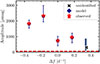 |
Fig. D.1. Same as Fig. 1 but for the four observed components of the quadrupole p-mode. |
| In the text | |
|
Fig. E.1. Magnetic sensitivity kernel of an example g mode with n = −1, l = 2. Magnetic sensitivity kernel of an example g mode with n = −1, l = 2. |
| In the text | |
|
Fig. E.2. Magnetic stress tensor of an example magnetic field used following the prescription of Duez & Mathis (2010). |
| In the text | |
Current usage metrics show cumulative count of Article Views (full-text article views including HTML views, PDF and ePub downloads, according to the available data) and Abstracts Views on Vision4Press platform.
Data correspond to usage on the plateform after 2015. The current usage metrics is available 48-96 hours after online publication and is updated daily on week days.
Initial download of the metrics may take a while.