| Issue |
A&A
Volume 704, December 2025
|
|
|---|---|---|
| Article Number | A336 | |
| Number of page(s) | 8 | |
| Section | Stellar structure and evolution | |
| DOI | https://doi.org/10.1051/0004-6361/202557247 | |
| Published online | 19 December 2025 | |
Is a 1D perturbative method sufficient for asteroseismic modelling of β Cephei pulsators?
Implications for measurements of rotation and internal magnetic fields
1
Université Paris-Saclay, Université de Paris, Sorbonne Paris Cité, CEA, CNRS, AIM, 91191 Gif-sur-Yvette, France
2
Institute of Astronomy, KU Leuven, Celestijnenlaan 200D, B-3001 Leuven, Belgium
3
Institute of Science and Technology Austria (ISTA), Am Campus 1, Klosterneuburg, Austria
4
Center for Astrophysics | Harvard & Smithsonian, 60 Garden Street, Cambridge, MA 02138, USA
5
IRAP, Université de Toulouse, CNRS, UPS, CNES, 14 avenue Édouard Belin, F-31400 Toulouse, France
6
Department of Astrophysics, IMAPP, Radboud University Nijmegen, PO Box 9010 6500 GL Nijmegen, The Netherlands
7
Max Planck Institute for Astronomy, Königstuhl 17, 69117 Heidelberg, Germany
8
LIRA, Observatoire de Paris, Université PSL, Sorbonne Université, Université Paris Cité, CY Cergy Paris Université, CNRS, 92190 Meudon, France
★ Corresponding author: This email address is being protected from spambots. You need JavaScript enabled to view it.
Received:
15
September
2025
Accepted:
10
November
2025
Abstract
Context. Asymmetries in the observed rotational splittings of a multiplet contain information about the star’s rotation profile and internal magnetic field. Moreover, the frequency regularities of multiplets can be used for mode identification. However, to exploit this information, highly accurate theoretical predictions are needed.
Aims. We aim to quantify the difference in the predicted mode asymmetries between a 1D perturbative method and a 2D method that includes a 2D stellar structure model, which takes rotation into account. We then place these differences between 1D and 2D methods in the context of asteroseismic measurements of internal magnetic fields. We only focus on the asymmetries and not on possible additional frequency peaks that can arise when the magnetic and rotation axis are misaligned.
Methods. We coupled the 1D pulsation codes GYRE and StORM to the 2D stellar structure code ESTER and compared the oscillation predictions with the results from the 2D TOP pulsation code. We focused on zero-age main-sequence models representative of rotating β Cephei pulsators spinning at up to 20 per cent of the critical Keplerian rotation rate. Specifically, we investigated low-radial-order gravity and pressure modes.
Results. We find a generally good agreement between the oscillation frequencies resulting from the 1D and 2D pulsation codes. We report differences in predicted mode multiplet asymmetries of mostly below 0.06 d−1. Since the magnetic asymmetries are small compared to the differences in the rotational asymmetries resulting from the 1D and 2D predictions, accurate measurements of the magnetic field are in most cases challenging.
Conclusions. Differences in the predicted mode asymmetries of a rotating star between 1D perturbative methods and 2D non-perturbative methods can greatly hinder accurate measurements of internal magnetic fields in main-sequence pulsators with low-order modes. Nevertheless, reasonably accurate measurements could be possible with npg ≥ 2 modes if the internal rotation is roughly below 10 per cent of the Keplerian critical rotation frequency for (aligned) magnetic fields of the order of a few hundred kilogauss. While the differences between the 1D and 2D frequency predictions are mostly too large for internal magnetic field detections, the rotational asymmetries predicted by StORM are in general accurate enough for asteroseismic modelling of the stellar rotation in main-sequence stars with identified low-order modes.
Key words: asteroseismology / stars: interiors / stars: magnetic field / stars: massive / stars: rotation
© The Authors 2025
 Open Access article, published by EDP Sciences, under the terms of the Creative Commons Attribution License (https://creativecommons.org/licenses/by/4.0), which permits unrestricted use, distribution, and reproduction in any medium, provided the original work is properly cited.
This article is published in open access under the Subscribe to Open model. This email address is being protected from spambots. You need JavaScript enabled to view it. to support open access publication.
1. Introduction
In the absence of stellar rotation or magnetism, the frequencies of stellar pulsation modes of equal spherical degree (ℓ) and radial order (npg) are degenerate for different azimuthal orders (m). This degeneracy in frequency is lifted by rotation, splitting a single frequency into a multiplet of 2ℓ+1 components. Up to the first order in the rotation frequency (Ω), the splitting is symmetric, namely ωm = ω0 + m(1 − Cℓ, n)Ω, where ωm is the frequency in the inertial frame and Cℓ, n is the Ledoux constant (Ledoux 1951). Higher-order effects also occur due to the Coriolis force and the centrifugal deformation of the mode cavities (e.g. Saio 1981; Gough & Thompson 1990; Goode & Thompson 1992; Soufi et al. 1998; Karami 2008; Guo et al. 2024, second and third order). The non-zonal (m ≠ 0) modes are more sensitive to the (rotational) equator and therefore experience a larger frequency shift compared to the zonal mode. This introduces asymmetries in the frequency splittings. Likewise, the presence of a magnetic field introduces asymmetries in the splittings (Loi 2020; Gomes & Lopes 2020; Bugnet et al. 2021; Mathis et al. 2021; Bugnet 2022; Li et al. 2022; Mathis & Bugnet 2023; Das et al. 2020, 2024). Such observed asymmetries have been exploited to estimate internal magnetic field strengths in red giants where the contribution of rotation to the asymmetry can be neglected, following the framework developed by Li et al. (2022) and used in follow-up studies (Li et al. 2023; Hatt et al. 2024).
For main-sequence pulsators that show frequency asymmetries, such as the β Cephei and δ Scuti pulsators, rotation cannot simply be neglected, but we note that these two classes of stars are typically in different regimes in terms of the fraction of critical rotation (see e.g. Huang et al. 2010) and in terms of excited radial orders. It is therefore crucial to have a good understanding of the effects of rotation on the asymmetries. Here, we focus on β Cephei pulsators. Mode identification of these stars starts to become feasible on a large scale from the analyses of combined photometry from the Gaia and Transiting Exoplanet Survey Satellite (TESS) missions (e.g. Gaia Collaboration 2023; Hey & Aerts 2024; Fritzewski et al. 2025). In the context of predicting mode asymmetries, all studies so far have relied on 1D perturbative methods. The 1D perturbative theory has been compared with 2D methods using polytropic models by Reese et al. (2006) for pressure modes (p modes), and by Ballot et al. (2010) for gravity modes (g modes). Furthermore, Burke et al. (2011) used realistic stellar structure models of stars of 1 and 2 M⊙, computed with the 1D ASTEC code (Christensen-Dalsgaard 2008), to compare the 1D and 2D methods. The validity domains of the perturbative method provided by these studies are based on the typical frequency resolution of the Convection Rotation and Planetary Transists (CoRoT) mission (Auvergne et al. 2009).
Asteroseismic modelling of real stars in 2D has been done for rapidly-rotating pulsators using both 2D steady models computed with the ESTER stellar structure and evolution code (Espinosa Lara & Rieutord 2013; Rieutord et al. 2016) coupled to the 2D stellar pulsation code (Reese et al. 2009). Such modelling efforts typically rely on the mode visibility for the mode identification, that is, the surface pressure perturbation integrated over the visible disc (Rieutord et al. 2024). However, 2D pulsation codes have never (to our knowledge) been used to reproduce pulsation spectra of slow rotators.
In this paper we quantify the difference in mode frequencies and rotationally split multiplet asymmetries of low-radial-order g and p modes predicted by the new 1D pulsation code (StORM) and a 2D pulsation code (TOP) for models representative of β Cephei pulsators. We ignore additional frequencies that can occur in multiplets if the magnetic and rotation axis are sufficiently misaligned. This can give rise to (2ℓ+1)2 frequencies in the inertial frame (Loi 2021), and additional frequencies in multiplets have been observed in some β Cephei pulsators (e.g. Shibahashi & Aerts 2000; Vanlaer et al. 2025a; Vandersnickt et al. 2025).
For the 2D case, we also used a 2D stellar structure model with a differential rotation profile resulting from the baroclinic torque and compared this model with the 1D case when solid body rotation is assumed (see also Houdayer & Reese 2023 for a comparison between a differentially rotating ESTER model and a deformed uniformly rotating one). Figure 1 shows an example of the 2D rotation profile, both for the zero-age main-sequence (ZAMS) model rotating at 10 per cent of the critical Keplerian rotation frequency (discussed in Sect. 2) and for the more evolved model (discussed in Sect. 5). From an observational point of view, we seek answers to two questions: (1) whether StORM is capable of predicting proper frequencies for low-order modes from its perturbative treatment of the rotational deformation of the star, and (2) when 1D asteroseismic modelling is performed and any residuals in the mode asymmetries are attributed to the presence of a magnetic field, how accurate would a magnetic field measurement then be. In Sect. 2 we discuss the numerical setup and work flow, in Sect. 3 we discuss the differences between 1D and 2D methods for ZAMS models, and we discuss the implications for measuring internal magnetic fields in Sect. 4. Furthermore, in Sect. 5 we discuss the effects of the nuclear evolution during the main sequence on our results, and we conclude in Sect. 6.
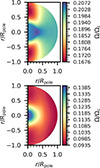 |
Fig. 1. Differential rotation profiles of a 12 M⊙ star computed with ESTER at ZAMS (top panel) and Xc = 0.4 (bottom panel), normalized by the critical rotation frequency at the equator. |
2. Numerical setup
We computed steady state models using the 2D stellar structure and evolution code ESTER1, r23.09.1-evol (Espinosa Lara & Rieutord 2013; Rieutord et al. 2016; Mombarg et al. 2023). We limited ourselves to chemically homogeneous ZAMS models, which we computed for a 12 M⊙ star and rotation rates of 0, 5, 10, 15, and 20 per cent of the critical Keplerian rotation frequency,  . Our argument not to go beyond this rotation regime for the time being is twofold. From an astrophysical standpoint, the population study of more than a hundred β Cephei pulsators carried out by Fritzewski et al. (2025) shows that their distribution of v/vc, Kep peaks around 0.2. The practical reason is that we can no longer unambiguously identify the corresponding mode frequencies between the 1D and 2D pulsation calculations for rotation rates above v/vc, Kep = 0.2. Table 1 provides a summary of the deformation and rotation velocities. The mass of 12 M⊙ is chosen to be close to the asteroseismically inferred mass of the β Cephei pulsator HD192575 (Burssens et al. 2023; Vanlaer et al. 2025a). Mode multiplets have been identified in the pulsation spectrum of this star for modes of spherical degree ℓ = 1 and 2. The rich pulsation spectrum of HD192575 makes it a prime target for modelling the interior rotation profile (Vanlaer et al. 2025a) and possibly measuring the internal magnetic field strength.
Ratio radius at the pole compared to the radius at the equator for ESTER models with different rotation rates.
2.1. 2D computations with TOP
The TOP code can directly take an ESTER model as input and uses the same spatially meshed grid, as the solvers of both codes are based on spectral methods. The ESTER grid is based on a multi-domain approach to deal with strong variations and possible discontinuities (in the radial direction) in the solution. Within each domain, the stellar quantities are sampled over the Gauss-Lobatto collocation points associated with Chebyshev polynomials, with appropriate interface conditions between the domains (Rieutord et al. 2016). The first domain is placed over the convective core, and the boundaries of the other domains are placed such that the pressure or temperature ratio between the inner and outer boundary remains roughly constant across domains.
We also coupled the 1D pulsation code GYRE (Townsend & Teitler 2013) to the non-rotating ESTER model. For the GYRE computations, we assumed a uniform rotation profile, where the traditional approximation of rotation is used for the g modes and the Coriolis force is neglected for the p modes. It should be noted that GYRE (and StORM) assumes a mass distribution that is only dependent on the radius, which is not the case for rotating 2D models. In Fig. 2 we show the resulting frequency differences when the number of radial points of the ESTER grid (same as the TOP grid) is increased. Fixing the number of domains – bounded by isobars – equal to 12, the differences are less than 10−5 d−1 when the radial resolution is further increased from 60 points per domain to 90. For the 1D finite differences codes, the relevant physical quantities from ESTER are interpolated to 2000 points in the radial direction. We only coupled non-rotating ESTER models to the 1D pulsation codes by generating a GYRE Stellar Model (GSM)2 from the ESTER models using the interpolated quantities in an arbitrary θ-direction. StORM is also compatible with this GSM format.
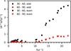 |
Fig. 2. Frequency differences for different radial resolutions of the ESTER and TOP grid. Frequency differences between 30 and 60 radial points per domain are in black, and differences between 60 and 90 points per domain in red. |
file format. In Fig. 3 we compare the frequency spectra of TOP and StORM (see Sect. 2.2) for ℓ ∈ [0, 1, 2, 3] computed from a non-rotating ESTER model. We find excellent agreement between the output of the two codes, with frequency differences between 8 ⋅ 10−6 and 0.0023 d−1. Similar frequency differences are found between TOP and GYRE (dotted red lines in the bottom panel of Fig. 3).
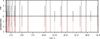 |
Fig. 3. Frequency spectra of a non-rotating ESTER model computed with TOP (top) and StORM (bottom). The GYRE frequency spectrum is indicated with dotted red lines. The ordinate corresponds to the value of ℓ. The radial modes are indicated with dashed black lines. |
Rotation couples modes of different ℓ and npg, and therefore, mode labelling in 2D is not trivial, making it challenging to identify modes belonging to the same multiplet as the mode spectrum is a priori infinitely dense in the gravito-inertial range of frequencies. Below, we describe our workflow to extract the mode splittings and their asymmetries.
-
Using GYRE, we scanned a frequency interval such that all radial orders of interest are contained.
-
Using TOP, we scanned this frequency interval using a low angular resolution nθ = 2, where the highest spherical degree taken into account in the coupling is given by ℓmax = |m|+2nθ. TOP requires a frequency shift around which the code should find nsol eigenmodes. We scanned the interval of 1–6.5 d−1 in steps of 0.5 d−1 and 10–20 d−1 in steps of 2 d−1, requesting three eigenmodes per frequency shift. The low-resolution mode enabled us to identify the locations of the large-scale modes that we were interested in, while saving CPU time.
-
Since the frequencies and eigenvectors of these large-scale modes are not fully resolved with this resolution, we scanned again around the found frequencies but with a higher resolution, nθ = 10. With this higher resolution, however, small-scale modes are also found close to the large-scale mode.
-
In order to filter out these small-scale modes from the large-scale ones, we assigned a ‘pseudo’
 and
and  , by simply counting the number of nodes in the radial and angular directions. It should be noted that this way of mode labelling is more ad hoc compared to that used by Mirouh et al. (2019) to label island modes, as the number of nodes may depend on the radius where we do the counting. Nevertheless, we find that in most cases
  allows us to identify the multiplets, where nnodes, θ is the number of nodes in the θ-direction over both hemispheres3. We then filtered out all modes
  and
and  .
. -
Lastly, we matched the remaining modes with the labelled ones from GYRE by simply selecting the mode with the same m that has a frequency difference below a certain threshold. Once we identified the multiplets in the TOP spectrum, we could compute the mode asymmetries.
The modes computed by TOP are classified as either ‘even’ (i.e. symmetric around the equator) or ‘odd’ (anti-asymmetric around the equator). In the case of ℓ = 1, the m = 0 modes are odd, and the m = ±1 modes are even. Likewise, for ℓ = 2, the m = 0 and m = ±2 modes are even, and the m = ±1 modes are odd.
2.2. 1D computations with StORM
We also computed the frequencies with the newly developed 1D StORM code4 (Vanlaer et al. 2025b). StORM solves the adiabatic oscillation equations, including the effects of rotation. It includes the Coriolis acceleration and a perturbative approximation for the centrifugal deformation of the star. This is accomplished in two steps. First, the oscillation equations are solved directly for a single spherical degree, only including the Coriolis acceleration terms. Second, the solutions from the simplified oscillation equations are perturbed taking the stellar deformation into account, as well as the coupling between different spherical degrees due to the contribution of the Coriolis acceleration and the toroidal components (e.g. Saio 1981; Lee & Baraffe 1995). Since StORM uses a 1D stellar model as input, the stellar deformation is approximated using the Chandrasekhar-Milne expansion up to the P2 term (Chandrasekhar 1933). It should be noted that the 1D computations with StORM are much faster than the 2D computations with TOP (of the order of seconds compared to the ∼30 min total computation time on four CPUs for our case when scanning the entire frequency range for even or odd modes).
3. Mode asymmetries
In this section we compare the predicted mode asymmetries of StORM and TOP. We computed mode asymmetries for ℓ ∈ [1, 2] and npg ∈ [ − 5, −4, −3, −2, −1, 0, 1, 2], corresponding to typically observed values in β Cephei pulsators (Stankov & Handler 2005; Fritzewski et al. 2025). The computations of StORM were done for a non-rotating ESTER model, where we considered the rotational effect only in the pulsation computations. We did so by taking a uniform rotation profile with equal fraction of the critical rotation frequency compared to the rotating ESTER model. The computations with TOP use the differential rotation profile that follows from the baroclinic torque as computed by ESTER (Espinosa Lara & Rieutord 2013).
We defined the relative asymmetry parameter as follows,
 (1)
(1)
where f−m < f0 < f+m (m > 0 for prograde modes). The results are shown in Figs. 4 and 5. Overall the predictions between the 1D perturbative method and full 2D are in good agreement. The largest differences are observed for the p modes and increase with increasing rotation. We confirm that the asymmetries of the low-order ℓ = 1 modes are strictly positive, while negative asymmetries A1 occur for the ℓ = 2 p modes for rotation rates above 10 per cent of the critical rotation. In Fig. 5, the additional A2 asymmetry parameters are shown, which are also strictly positive. In some cases, particularly for the model with the highest rotation rate, some frequencies of a multiplet could not be clearly identified in the TOP frequency spectrum as a result of additional modes with similar frequency and a significant change in the eigenfunction compared to the eigenfunction for zero rotation.
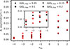 |
Fig. 4. Predicted asymmetry parameters (dimensionless) for ℓ = 1 computed with TOP (in black) and StORM (in red) as a function of radial order. |
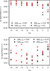 |
Fig. 5. Predicted asymmetry parameters for ℓ = 2 computed with TOP (in black) and StORM (in red) as a function of radial order. |
The differences in the asymmetries5 in units of d−1 (numerator in Eq. (1)) are shown in Fig. 6. We find that differences in the asymmetry are mostly limited to 0.06 d−1, and below 0.04 d−1 for rotation rates ≤15% of the critical rotation. This is within the realm of theoretical uncertainties on predictions of mode frequencies due to limited knowledge on the input physics of the models (Aerts et al. 2018). However, these uncertainties will be very similar for all the frequencies in Eq. (1) and thus will not hamper interpretations of asymmetries in observed mode multiplets of real stars. In absolute terms, these differences in asymmetries between TOP and StORM predictions are smaller than the actual measured rotation frequency of β Cephei pulsators; as such, identifications of m-values are also not an issue in practice except perhaps for the slowest rotators, such as HD 129929 (Aerts et al. 2003; Dupret et al. 2004). In most cases, the difference  is positive, meaning the 1D method in general tends to underestimate the asymmetries.
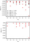 |
Fig. 6. Differences in the predicted asymmetry (TOP – StORM) as a function of radial order. Black symbols corresponds to ℓ = 1, red symbols to ℓ = 2. |
We estimated the contribution of the radial differential rotation (2D method) versus uniform rotation (1D setup) to the total differences in frequencies by evaluating  , where
  is the average rotation frequency. For our models used in this work, α < 0.1, meaning that we do not expect that the difference in the rotation profile between the 1D and 2D method has a very large effect.
4. Effect on measurements of magnetic fields
In this section we quantify what the differences in mode asymmetries predicted from 1D or 2D methods could imply for the detection and measurement of an internal magnetic field. If an internal magnetic field is invoked to explain any residuals in observed asymmetries after correcting for the rotation, what would be the difference in the measured magnetic field characteristics originating from the differences between the 1D and 2D frequency predictions adopted for the rotational asymmetry part?
The computation of the magnetic asymmetries are computed with the magsplitpy code, and we refer the reader to Das et al. (2024) for the details of the code. The code uses the same description for the magnetic field topology as outlined in Prat et al. (2019) and Bugnet et al. (2021). The chosen field configuration, initially derived in Duez & Mathis (2010), is composed of poloidal and toroidal components and so the magnetic field is stable over evolutionary timescales. However, unlike in Bugnet et al. (2021), where the magnetic field beyond the radiative core is zero for their application to red giant stars, we extended the field all the way through the envelope (vanishing at the stellar surface), as the modes studied here are sensitive to larger portion of the star. The magnetic asymmetries are computed for different inclinations of the field with respect to the star’s rotation axis, referred to as the obliquity angle, β, which is known to crucially modulate the magnetic asymmetries as shown in Loi (2021), Li et al. (2022), Mathis & Bugnet (2023), and Das et al. (2024).
The magnetic asymmetries scale with amplitude of the magnetic field squared,  (for the assumed topology of the magnetic field). Therefore, for a given multiplet and field obliquity angle β, the amplitude of the magnetic field can be over- or underestimated if the calculated asymmetry resulting from rotation is inaccurate. For example, a difference in the asymmetry (
 ) between 1D and 2D methods will result in a difference of the measured magnetic field,
 (2)
(2)
where B0′−B0 is the error6 on the inferred field strength when relying on 1D perturbative methods to treat the rotational effects. From an observational point of view,  represents the residual asymmetry after accounting for the rotation, which is then assumed to be the result of magnetic effects. Hence, when
  , measurements of the field strength will be overestimated. As the obliquity angle increases, the magnetic asymmetries for a dipolar field will decrease until a critical angle ∼55° where there is a change of sign (Li et al. 2022; Mathis & Bugnet 2023; Das et al. 2024). Therefore, accurate measurement of B0 when β is close to this critical value is impossible, as is shown in Fig. 7. In the example shown in this figure, B0 = 1 MG, which gives large enough
  to prevent the contribution of
  from flipping the sign.
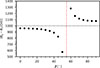 |
Fig. 7. Difference between the measured magnetic field strength (B0′) and the actual one (B0 = 1 MG) as a function of the obliquity angle (β). Here, A1 asymmetries were used for npg = 2, and |

We next quantified the error on the inferred B0 when β = 0° for each of the radial orders for which we could determine  . The magnetic asymmetries were computed with magsplitpy for B0 = 75 kG. We used
  to scale the asymmetries to any value of the magnetic field strength. Figure 8 shows the error of the measured magnetic field strength as a function of the actual one for the most optimistic case, namely npg = 2. In this case, field strengths above ∼300 kG could be measured with an error better than 50 per cent, and field strengths above ∼700 kG could be measured with an error better than 10 per cent. For comparison, measured surface magnetic field strengths for O types are typically of the order of a few kilogauss, and ∼4–10 kG for early B-type stars (Shultz et al. 2019). We note that this minimum B0 scales inversely with the fraction of critical rotation. The range of B0 covered in Fig. 8 is simply chosen to cover a large range and the higher values may be higher than what is typical for real stars. The lower end points of the curves indicate where the square-root term in Eq. (1) becomes negative. For the other radial orders npg ∈ [ − 5, …, 1], the predicted magnetic asymmetries of this ESTER ZAMS model are so small that even at 0.05 Ω/Ωc, Kep the uncertainty on the rotational asymmetry prevents any magnetic field measurement below 1 MG with reasonable uncertainty. Therefore, even though the difference in the predicted rotational asymmetry between 1D and 2D methods is larger in low-order p modes compared to low-order g modes, the magnetic asymmetries are also larger and scale in such a way that modes with npg ≥ 2 provide the best diagnostic for potential measurements of internal magnetic fields in β Cephei stars.
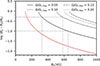 |
Fig. 8. Error of the measured magnetic field strength as a function of the actual magnetic strength. The black curves correspond to A1 asymmetries (ℓ = 1), the red curve to A2 asymmetries. Field strength fractional errors corresponding to 50% and 10% are indicated with dashed grey lines. |
5. Effect of nuclear evolution on the asymmetries
We then investigated how dependent the results presented in the previous sections were on the effect of the nuclear evolution during the main sequence. Achieving nuclear evolution with ESTER with sufficient mesh resolution for the pulsation computations is numerically challenging and time consuming7. We evolved a 12 M⊙ star with ESTER up to a central hydrogen mass fraction of Xc ≈ 0.4, once for a non-rotating star and once for an initial rotation rate 0.1 Ω/Ωc, Kep (at the ZAMS). Such an evolutionary stage (Xc) is representative for the sample of β Cephei pulsators of Fritzewski et al. (2025). The r23.09.1-evol release of ESTER that we used for this treats chemical mixing in the radiative envelope based on the work of Zahn (1992) with a prescribed vertical eddy-viscosity associated with the vertical shear, whereas for the non-rotating case a constant diffusion coefficient is used that we here set equal to 104 cm2 s−1, based on measurements of Pedersen et al. (2021). Therefore, there are some small differences in the stellar structure between the rotating and non-rotating model, but this should have a minimal effect on the mode asymmetries as the two models are still very similar in structure (fractional convective core mass of 0.2532 and 0.2501, respectively).
Figure 9 shows the differences in the predicted asymmetries between 1D and 2D methods. While the model starts with a rotation rate of 0.1 Ωc, Kep at the ZAMS, the fraction of critical rotation decreases slightly, as is the case for ESTER models above ∼8 M⊙ (Mombarg et al. 2024). The evolved model that we took here rotates at 0.0942 Ωc, Kep. For comparison, the differences in asymmetries for the ZAMS model rotating at 0.1 Ωc, Kep are also shown. As can be seen from Fig. 9, similar differences are found for the more evolved model compared to the ZAMS model.
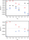 |
Fig. 9. Same as Fig. 6 but for a model with Xc ≈ 0.4. The fraction of critical rotation of this model is 0.0942 Ωc, Kep. Black symbols corresponds to ℓ = 1, red symbols to ℓ = 2. For comparison, the results from the ZAMS model at 0.1 Ωc, Kep from Fig. 6 are also shown in blue. |
Again, we investigated the implications for measurements of B0. The magnetic splittings and asymmetries depend on the product of the mode kernel and the Lorentz stress tensor BB. We find that the effect of the evolution of the stellar structure plays a bigger role for the magnetic asymmetries compared to the rotational ones. The magnetic asymmetries of the more evolved model that we studied here are about 4 to 18 times larger than those of the ZAMS model. In Fig. 10 we show the error of the measured B0 similar to Fig. 8. As can be seen, a magnetic field could be measured with a smaller error for the more evolved model, since the magnetic asymmetries become larger while the rotational ones remain similar. For the model rotating at 0.0942 Ωc, Kep, 50 per cent error could be achieved around 250 kG instead of 600 kG for the ZAMS model. Furthermore, we note that while for the ZAMS model the A2 (ℓ = 2) asymmetries would be more accurate compared to the A1 asymmetries, it is the other way around for the more evolved model.
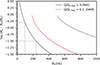 |
Fig. 10. Same as Fig. 8 but for a model at Xc = 0.4. For comparison, the results for the ZAMS model with a rotation rate of 0.1 Ω/Ωc, Kep are shown again here. |
6. Conclusion
In this paper we have compared a 1D perturbative method for computing eigenfrequencies of rotating stars with a non-perturbative 2D method (including 2D stellar equilibrium models). We have presented predicted mode asymmetries of the rotational splittings for 12 M⊙ ZAMS models, covering low-radial-order modes that are typically observed in β Cephei pulsators (e.g. Stankov & Handler 2005; Fritzewski et al. 2025). We computed asymmetries for rotation rates up to 20 per cent of the critical Keplerian rotation rate, above which it becomes difficult to identify multiplets in the predicted mode spectra of the g modes. We show that the sign of the asymmetries is consistent between the 1D and 2D methods and, therefore, that stars with asymmetries of an opposite sign could indicate the presence of a magnetic field.
We have shown that when residual observed asymmetries – after accounting for rotational effects with 1D methods – are assumed to come from magnetic effects, the resulting measured magnetic field strength can change by orders of magnitude between the 1D and 2D methods used for the rotation, even when the centrifugal deformation is minimal. However, we find that reasonably accurate measurements of the magnetic field strength are in principle possible for npg = 2 (and likely higher radial orders, although higher radial orders are unlikely to be excited) when the fraction of critical rotation is not more than 10 per cent and the magnetic field strength is high enough (at least ≳300 kG).
As shown in this work, accurate measurements of an internal magnetic field that rely on 1D perturbative methods to treat the rotation are extremely limited. This of course does not imply that such methods have no scientific use. The StORM code that we used here is able to reproduce rotational asymmetries with an adequate precision in a fast manner. This makes it a valuable tool for asteroseismic measurements of rotational properties, with the capacity to treat large samples of stars. StORM’s 1D perturbative approach for the centrifugal deformation provides appreciably better accuracy over current state-of-the-art pulsation codes that do not account for this deformation. We do note, however, that the detection (which is not necessarily equal to an accurate measurement) of an internal misaligned magnetic field in β Cephei pulsators can be achieved by means of detecting additional peaks in multiplets.
Data availability
The ESTER models and mode asymmetries are available on Zenodo: https://zenodo.org/records/17580179
Where possible, manual mode identification was done for a few cases with unsuccessful frequency correspondence by visually inspecting the eigenfunction of candidate modes.
We use a tilde to distinguish between the dimensionless asymmetry (A) and the asymmetry in units of frequency ( ).
).
The terms ‘error’ and ‘uncertainty’ mentioned here refer to over- or underestimation of the magnetic field strength between 1D and 2D methods for the rotation. This should not be confused with an observational measurement precision.
To reduce the number of steps needed to reach convergence, we relaxed the default tolerance by a factor of 5.
Acknowledgments
We thank the anonymous referee for their comments on the manuscript, Dario Fritzewski for providing the distribution of fractions of critical rotation for the β Cephei sample, and Zhao Guo for the discussions. The research leading to these results has received funding from the European Research Council (ERC) under the Horizon Europe programme (Synergy Grant agreement N°101071505: 4D-STAR). While partially funded by the European Union, views and opinions expressed are however those of the authors only and do not necessarily reflect those of the European Union or the European Research Council. Neither the European Union nor the granting authority can be held responsible for them. V.V. acknowledges support from the Research Foundation Flanders (FWO) under grant agreement N°1156923N (PhD Fellowship). S.B.D. acknowledges funding from the European Union’s Horizon 2020 research and innovation programme under the Marie Skłodowska-Curie grant agreement N°101034413. L.B. gratefully acknowledges support from the European Research Council (ERC) under the Horizon Europe programme (Calcifer; Starting Grant agreement N°101165631). J.B., M.R., S.M. and J.S.G.M have been supported by CNES, focused on the preparation of the PLATO mission. Computations with ESTER and TOP have made use of the HPC resources from the CALMIP supercomputing centre (Grant 2023-P0107). This research made use of the numpy (Harris et al. 2020) and matplotlib (Hunter 2007) Python software packages.
References
- Aerts, C., Thoul, A., Daszyńska, J., et al. 2003, Science, 300, 1926 [Google Scholar]
- Aerts, C., Molenberghs, G., Michielsen, M., et al. 2018, ApJS, 237, 15 [Google Scholar]
- Auvergne, M., Bodin, P., Boisnard, L., et al. 2009, A&A, 506, 411 [NASA ADS] [CrossRef] [EDP Sciences] [Google Scholar]
- Ballot, J., Lignières, F., Reese, D. R., & Rieutord, M. 2010, A&A, 518, A30 [NASA ADS] [CrossRef] [EDP Sciences] [Google Scholar]
- Bugnet, L. 2022, A&A, 667, A68 [NASA ADS] [CrossRef] [EDP Sciences] [Google Scholar]
- Bugnet, L., Prat, V., Mathis, S., et al. 2021, A&A, 650, A53 [NASA ADS] [CrossRef] [EDP Sciences] [Google Scholar]
- Burke, K. D., Reese, D. R., & Thompson, M. J. 2011, MNRAS, 414, 1119 [Google Scholar]
- Burssens, S., Bowman, D. M., Michielsen, M., et al. 2023, Nat. Astron., 7, 913 [NASA ADS] [CrossRef] [Google Scholar]
- Chandrasekhar, S. 1933, MNRAS, 93, 390 [NASA ADS] [CrossRef] [Google Scholar]
- Christensen-Dalsgaard, J. 2008, Ap&SS, 316, 13 [Google Scholar]
- Das, S. B., Chakraborty, T., Hanasoge, S. M., & Tromp, J. 2020, ApJ, 897, 38 [NASA ADS] [CrossRef] [Google Scholar]
- Das, S. B., Einramhof, L., & Bugnet, L. 2024, A&A, 690, A217 [NASA ADS] [CrossRef] [EDP Sciences] [Google Scholar]
- Duez, V., & Mathis, S. 2010, A&A, 517, A58 [NASA ADS] [CrossRef] [EDP Sciences] [Google Scholar]
- Dupret, M. A., Thoul, A., Scuflaire, R., et al. 2004, A&A, 415, 251 [NASA ADS] [CrossRef] [EDP Sciences] [Google Scholar]
- Espinosa Lara, F., & Rieutord, M. 2013, A&A, 552, A35 [NASA ADS] [CrossRef] [EDP Sciences] [Google Scholar]
- Fritzewski, D. J., Vanrespaille, M., Aerts, C., et al. 2025, A&A, 698, A253 [NASA ADS] [CrossRef] [EDP Sciences] [Google Scholar]
- Gaia Collaboration (De Ridder, J., et al.) 2023, A&A, 674, A36 [CrossRef] [EDP Sciences] [Google Scholar]
- Gomes, P., & Lopes, I. 2020, MNRAS, 496, 620 [NASA ADS] [CrossRef] [Google Scholar]
- Goode, P. R., & Thompson, M. J. 1992, ApJ, 395, 307 [Google Scholar]
- Gough, D. O., & Thompson, M. J. 1990, MNRAS, 242, 25 [Google Scholar]
- Guo, Z., Bedding, T. R., Pamyatnykh, A. A., et al. 2024, MNRAS, 535, 2927 [Google Scholar]
- Harris, C. R., Millman, K. J., van der Walt, S. J., et al. 2020, Nature, 585, 357 [NASA ADS] [CrossRef] [Google Scholar]
- Hatt, E. J., Ong, J. M. J., Nielsen, M. B., et al. 2024, MNRAS, 534, 1060 [NASA ADS] [CrossRef] [Google Scholar]
- Hey, D., & Aerts, C. 2024, A&A, 688, A93 [NASA ADS] [CrossRef] [EDP Sciences] [Google Scholar]
- Houdayer, P. S., & Reese, D. R. 2023, A&A, 675, A181 [NASA ADS] [CrossRef] [EDP Sciences] [Google Scholar]
- Huang, W., Gies, D. R., & McSwain, M. V. 2010, ApJ, 722, 605 [Google Scholar]
- Hunter, J. D. 2007, Comput. Sci. Eng., 9, 90 [NASA ADS] [CrossRef] [Google Scholar]
- Karami, K. 2008, Chin. J. Astron. Astrophys., 8, 285 [NASA ADS] [CrossRef] [Google Scholar]
- Ledoux, P. 1951, ApJ, 114, 373 [Google Scholar]
- Lee, U., & Baraffe, I. 1995, A&A, 301, 419 [NASA ADS] [Google Scholar]
- Li, G., Deheuvels, S., Ballot, J., & Lignières, F. 2022, Nature, 610, 43 [NASA ADS] [CrossRef] [Google Scholar]
- Li, G., Deheuvels, S., Li, T., Ballot, J., & Lignières, F. 2023, A&A, 680, A26 [NASA ADS] [CrossRef] [EDP Sciences] [Google Scholar]
- Loi, S. T. 2020, MNRAS, 496, 3829 [Google Scholar]
- Loi, S. T. 2021, MNRAS, 504, 3711 [NASA ADS] [CrossRef] [Google Scholar]
- Mathis, S., & Bugnet, L. 2023, A&A, 676, L9 [NASA ADS] [CrossRef] [EDP Sciences] [Google Scholar]
- Mathis, S., Bugnet, L., Prat, V., et al. 2021, A&A, 647, A122 [EDP Sciences] [Google Scholar]
- Mirouh, G. M., Angelou, G. C., Reese, D. R., & Costa, G. 2019, MNRAS, 483, L28 [NASA ADS] [CrossRef] [Google Scholar]
- Mombarg, J. S. G., Rieutord, M., & Espinosa Lara, F. 2023, A&A, 677, L5 [NASA ADS] [CrossRef] [EDP Sciences] [Google Scholar]
- Mombarg, J. S. G., Rieutord, M., & Espinosa Lara, F. 2024, A&A, 683, A94 [NASA ADS] [CrossRef] [EDP Sciences] [Google Scholar]
- Pedersen, M. G., Aerts, C., Pápics, P. I., et al. 2021, Nat. Astron., 5, 715 [NASA ADS] [CrossRef] [Google Scholar]
- Prat, V., Mathis, S., Buysschaert, B., et al. 2019, A&A, 627, A64 [NASA ADS] [CrossRef] [EDP Sciences] [Google Scholar]
- Reese, D., Lignières, F., & Rieutord, M. 2006, A&A, 455, 621 [NASA ADS] [CrossRef] [EDP Sciences] [Google Scholar]
- Reese, D. R., MacGregor, K. B., Jackson, S., Skumanich, A., & Metcalfe, T. S. 2009, A&A, 506, 189 [NASA ADS] [CrossRef] [EDP Sciences] [Google Scholar]
- Rieutord, M., Espinosa Lara, F., & Putigny, B. 2016, J. Comput. Phys., 318, 277 [NASA ADS] [CrossRef] [Google Scholar]
- Rieutord, M., Reese, D. R., Mombarg, J. S. G., & Charpinet, S. 2024, A&A, 687, A259 [NASA ADS] [CrossRef] [EDP Sciences] [Google Scholar]
- Saio, H. 1981, ApJ, 244, 299 [NASA ADS] [CrossRef] [Google Scholar]
- Shibahashi, H., & Aerts, C. 2000, ApJ, 531, L143 [NASA ADS] [CrossRef] [Google Scholar]
- Shultz, M. E., Wade, G. A., Rivinius, T., et al. 2019, MNRAS, 490, 274 [NASA ADS] [CrossRef] [Google Scholar]
- Soufi, F., Goupil, M. J., & Dziembowski, W. A. 1998, A&A, 334, 911 [NASA ADS] [Google Scholar]
- Stankov, A., & Handler, G. 2005, ApJS, 158, 193 [NASA ADS] [CrossRef] [Google Scholar]
- Townsend, R. H. D., & Teitler, S. A. 2013, MNRAS, 435, 3406 [Google Scholar]
- Vandersnickt, J., Vanlaer, V., Vanrespaille, M., & Aerts, C. 2025, A&A, 704, L13 [NASA ADS] [CrossRef] [EDP Sciences] [Google Scholar]
- Vanlaer, V., Bowman, D. M., Burssens, S., et al. 2025a, A&A, 701, A5 [NASA ADS] [CrossRef] [EDP Sciences] [Google Scholar]
- Vanlaer, V., Mombarg, J. S. G., Guo, Z., & Townsend, R. H. D. 2025b, A&A, submitted [Google Scholar]
- Zahn, J. P. 1992, A&A, 265, 115 [NASA ADS] [Google Scholar]
All Tables
Ratio radius at the pole compared to the radius at the equator for ESTER models with different rotation rates.
All Figures
|
Fig. 1. Differential rotation profiles of a 12 M⊙ star computed with ESTER at ZAMS (top panel) and Xc = 0.4 (bottom panel), normalized by the critical rotation frequency at the equator. |
| In the text | |
|
Fig. 2. Frequency differences for different radial resolutions of the ESTER and TOP grid. Frequency differences between 30 and 60 radial points per domain are in black, and differences between 60 and 90 points per domain in red. |
| In the text | |
|
Fig. 3. Frequency spectra of a non-rotating ESTER model computed with TOP (top) and StORM (bottom). The GYRE frequency spectrum is indicated with dotted red lines. The ordinate corresponds to the value of ℓ. The radial modes are indicated with dashed black lines. |
| In the text | |
|
Fig. 4. Predicted asymmetry parameters (dimensionless) for ℓ = 1 computed with TOP (in black) and StORM (in red) as a function of radial order. |
| In the text | |
|
Fig. 5. Predicted asymmetry parameters for ℓ = 2 computed with TOP (in black) and StORM (in red) as a function of radial order. |
| In the text | |
|
Fig. 6. Differences in the predicted asymmetry (TOP – StORM) as a function of radial order. Black symbols corresponds to ℓ = 1, red symbols to ℓ = 2. |
| In the text | |
|
Fig. 7. Difference between the measured magnetic field strength (B0′) and the actual one (B0 = 1 MG) as a function of the obliquity angle (β). Here, A1 asymmetries were used for npg = 2, and |
| In the text | |
|
Fig. 8. Error of the measured magnetic field strength as a function of the actual magnetic strength. The black curves correspond to A1 asymmetries (ℓ = 1), the red curve to A2 asymmetries. Field strength fractional errors corresponding to 50% and 10% are indicated with dashed grey lines. |
| In the text | |
|
Fig. 9. Same as Fig. 6 but for a model with Xc ≈ 0.4. The fraction of critical rotation of this model is 0.0942 Ωc, Kep. Black symbols corresponds to ℓ = 1, red symbols to ℓ = 2. For comparison, the results from the ZAMS model at 0.1 Ωc, Kep from Fig. 6 are also shown in blue. |
| In the text | |
|
Fig. 10. Same as Fig. 8 but for a model at Xc = 0.4. For comparison, the results for the ZAMS model with a rotation rate of 0.1 Ω/Ωc, Kep are shown again here. |
| In the text | |
Current usage metrics show cumulative count of Article Views (full-text article views including HTML views, PDF and ePub downloads, according to the available data) and Abstracts Views on Vision4Press platform.
Data correspond to usage on the plateform after 2015. The current usage metrics is available 48-96 hours after online publication and is updated daily on week days.
Initial download of the metrics may take a while.