| Issue |
A&A
Volume 704, December 2025
|
|
|---|---|---|
| Article Number | L5 | |
| Number of page(s) | 4 | |
| Section | Letters to the Editor | |
| DOI | https://doi.org/10.1051/0004-6361/202557389 | |
| Published online | 02 December 2025 | |
Letter to the Editor
Manifestation of the stellar wind cycle in infrared images: Example of the heliosphere
1
Space Research Institute of Russian Academy of Sciences, Profsoyuznaya 84/32, Moscow 117997, Russia
2
Lomonosov Moscow State University, Leninskie Gory 1, Moscow 119991, Russia
3
HSE University, 20 Myasnitskaya Ulitsa, Moscow 101000, Russia
⋆ Corresponding author: This email address is being protected from spambots. You need JavaScript enabled to view it.
Received:
24
September
2025
Accepted:
13
November
2025
Abstract
Aims. The regions in which stellar winds interact with the interstellar medium, also known as astrospheres, can be observed in detail through the thermal emission of the interstellar dust particles, resided in plasma. Interstellar dust is also directly observed in the vicinity of the Sun with dust detectors onboard spacecraft, and it is known to be affected by the interplanetary magnetic field. The main goal of this work is to show how the change in the interplanetary magnetic field with the solar cycle affects the infrared picture of the heliosphere.
Methods. To compose a synthetic intensity map of the interstellar dust thermal emission, we used the Monte Carlo method to calculate the distribution of the dust particles inside the heliosphere. We considered the effects of the heliosphere boundaries and the non-stationary current sheet.
Results. The change in the Parker magnetic field caused by the solar activity cycle leads distinguishable features in the mid-infrared emission maps of the heliosphere. The distribution of the interstellar dust in the vicinity of the Sun we calculated suggests that small particles linger outside of the heliosphere, and medium-size particles are mostly affected by the changing interplanetary magnetic field, which leads to number density waves in the tail region of the heliosphere. Finally, large particles form a bulge behind the Sun.
Key words: Sun: activity / Sun: heliosphere / stars: activity / stars: winds / outflows / dust, extinction
© The Authors 2025
 Open Access article, published by EDP Sciences, under the terms of the Creative Commons Attribution License (https://creativecommons.org/licenses/by/4.0), which permits unrestricted use, distribution, and reproduction in any medium, provided the original work is properly cited.
This article is published in open access under the Subscribe to Open model. This email address is being protected from spambots. You need JavaScript enabled to view it. to support open access publication.
1. Introduction
The region of the solar wind is filled with plasma that expands from the surface of the Sun into the interstellar medium (ISM). Since the solar wind becomes supersonic at small distances and the Sun travels in the ISM at a speed that exceeds the local speed of sound, a complex structure arises that consists of two shock waves, the heliospheric shock wave (TS) and the bow shock (BS), and of tangential discontinuity, the heliopause (HP) (Baranov et al. 1970). This structure is called heliospheric boundary layer or shock layer. The plasma convects the interstellar magnetic field in the region outside of the HP. Inside the HP, it convects the solar magnetic field, forming the Parker spiral (Parker 1958).
Interstellar dust particles enter the heliospheric boundary layer and move under the effects of the gravitational attraction to the star, radiative pressure from stellar photons, the electromagnetic force, and the drag force. Smaller particles linger outside of the HP, while larger particles penetrate into the heliosphere. In- situ observations on spacecrafts, such as Ulysses (Grun et al. 1993) and Stardust (Westphal et al. 2014), confirmed the presence of interstellar dust particles in the vicinity of the Sun. The dynamics of the dust particles that move inside the heliosphere are affected by the interplanetary magnetic field (IMF)(Sterken et al. 2022; Baalmann et al. 2025), which itself has a dynamic structure.
The solar wind changes periodically with the 11-year activity cycle of the sunspots. During this cycle, the solar magnetic field changes polarity, which leads to the 22-year magnetic cycle and to alteration of the IMF. Since interstellar dust dynamics inside the heliosphere are governed by the IMF, the distribution of the interstellar dust particles in the heliosphere is affected by the solar activity (Godenko & Izmodenov 2024a).
Some other stars similar to the Sun are known to have a magnetic activity cycle. The chromospheric magnetic activity of distant stars is observed through the variation in the S index, which is an emission measure of the Ca II H and K lines (Baliunas et al. 1995). The challenging part of these observations is that they need to be conducted on long timescales. The Mount Wilson observations (Wilson 1978) collected one of the longest datasets on stellar activity over several decades. A number of datasets of long-term stellar activity observations are available today (see Jeffers et al. (2023) for a recent review). Nevertheless, only a few stars are confirmed to experience the polarity change at activity maxima like the Sun (Bellotti et al. 2025). The first stars to show a polarity change were Cygni A (Boro Saikia et al. 2016) and τ Bootis (Jeffers et al. 2018), with 7.3 yr and 10 yr cycles, respectively.
The shock layers of other stars are observed in the mid-infrared through the thermal radiation of interstellar dust particles that penetrate this shock layer and are heated by the star (Cox et al. 2012; Kobulnicky et al. 2016; Gvaramadze 2020; Larkin et al. 2025; Russeil et al. 2025). Some stars release dust into the ISM, and this dust can form circular shells around the stars (Drudis & Gvaramadze 2020). The interplanetary dust environment of the Sun is relatively dust poor in comparison to debris discs of other stars (Poppe et al. 2019), which, however, can make the interstellar dust prominent on the scale of the heliosphere.
Most current models of the interstellar dust distribution inside the heliosphere are intended to analyse the Ulysses data (Godenko & Izmodenov 2024b; Baalmann et al. 2025). Frisch & Slavin (2013) modelled the large-scale distribution of dust particles in the heliosphere using the heliosphere model of Pogorelov et al. (2008). They noted that large dust grains that penetrate the heliosphere are concentrated either at the solar equatorial plane during the focusing phase or in the polar region during the defocusing phase, but the authors only considered a stationary IMF. Alexashov et al. (2016) modelled the interstellar dust distribution with a non-stationary IMF, but mainly focused on the deflection of the dust at the heliosphere boundaries.
The goal of this Letter is to answer the question how the stellar cycle manifests itself in the infrared image of the astrosphere. For this purpose, we studied the interstellar dust distribution in the vicinity of the Sun and its effect on the infrared picture of the heliosphere. We used a numerical model of the interstellar dust distribution with a Monte Carlo approach that included the effect of the heliosphere boundaries and non-stationary IMF to compose synthetic mid-infrared emission maps of the heliosphere. The structure of the paper is as follows. In Section 2 we briefly describe the model. In Section 3 we present and discuss our results. Section 4 concludes this paper.
2. Methods
Interstellar dust particles are heated by the radiation of the Sun and emit thermal radiation. The emissivity of the potpourri of dust particles of different sizes can be expressed in the following form (Katushkina & Izmodenov 2019):
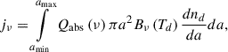 (1)
(1)
where a is the dust particle radius, Qabs is an absorption coefficient of the dust particle, Bν is the Plank function, Td is the dust particle temperature, dnd/da is the number density of the particles of sizes from a to a + da, and ν is the wave frequency.
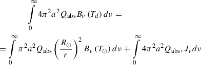
The spectral intensity from the dust grains can be derived by integrating the spectral emissivity along the line of sight,
 (2)
(2)
where s is the coordinate along the line of sight.
Typically, the thermal radiation of dust particles in the vicinity of other stars is observed in the mid-infrared. We chose ν0, which corresponds to the spectral emission maximum at the wavelength λ0 = 50 μm. We show intensity maps that represent the integrated emissivity along lines of sight parallel to the direction towards the observer and evenly spaced in the projection plane.
The absorption coefficient of the dust particles was calculated using Mie theory (Bohren & Huffman 1998). Since there is no in situ evidence of PAH and carbon particles inside the heliosphere, we restricted our calculations to the astronomical silicates. We employed the values of the absorption coefficient for the astronomical silicates obtained by Draine (2003).
The temperature of the dust particles was obtained via energy equilibrium between absorption of the interstellar and solar radiation field photons and emission of a single particle,
 (3)
(3)
where R⊙ is the radius of the Sun, T⊙ is the temperature of the Sun, r is the distance to the Sun, and Jν is the intensity of the isotropic interstellar radiation field.
The size distribution function of the dust particles was assumed to be homogeneous in the ISM,
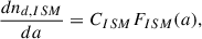 (4)
(4)
where FISM is the dust size distribution, and CISM is the factor that keeps the interstellar dust to the plasma mass density ratio ρd/ρp = 1/100.
To obtain the number density of the particles in the region that is disturbed by the Sun (i.e. inside the heliosphere boundary layer), we calculated the number density of particles of distinct size  , with the number density in the undisturbed medium set to unity. Then the number density inside the boundary layer was obtained as
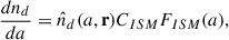 (5)
(5)
where r is the position of the particle, and  is the number density of the particles of distinct sizes.
To calculate the number density of particles of distinct sizes, we used the Monte Carlo method described in detail by Godenko & Izmodenov (2024b). We introduced the coordinate system so that the Z-axis was opposite to the direction of the velocity of the ISM, the X-axis was directed so that the homogeneous interstellar magnetic field vector lay in the XZ plane (BV plane), and the Y-axis completed the right-handed coordinate system (Fig. 1).
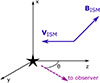 |
Fig. 1. Coordinate system used for calculations. The Sun is at the origin, VISM is the relative velocity of the interstellar dust and plasma, BISM is the interstellar magnetic field, and θ is an angle between the direction towards the observer and the velocity of the ISM. |
The Monte Carlo calculations were carried out in a rectangular box 1000 a.u. × 1000 a.u. × 1000 a.u., centred at the Sun. We used a regular rectangular grid, with 10 a.u. × 10 a.u. × 10 a.u. resolution in space and a one-year resolution in time. The boundary condition was set far from the heliosphere boundary layer in the undisturbed ISM, where all particles are assumed to move with the bulk velocity of the plasma. The plasma parameters and magnetic field strength inside the boundary layer were taken from a global MHD-kinetic model of the heliosphere (Izmodenov & Alexashov 2015, 2020). We considered a non-stationary heliospheric current sheet that propagates with plasma inside the heliosphere (see Godenko & Izmodenov 2024b, Appendix A).
For simplicity, the dust particles were assumed to have a constant mass and spherical shape. The charge of the particles was calculated according to the balance between the sticking of thermal plasma protons and electrons, secondary electron emission, photoelectric emission, and the effect of cosmic rays (see Godenko & Izmodenov 2023b).
The number density of the interstellar dust inside the heliosphere was calculated for astronomical silicates of sizes in between amin = 10 nm and amax = 1 μm. We used a standard power-law size distribution (Mathis et al. 1977) to model the thermal emission maps.
3. Results and discussion
Figure 2 shows the number density of particles of different sizes in the BV plane. Small particles (i.e. particles smaller than ≈100 nm) do not penetrate the heliosphere and stay in the outer shock layer (Fig. 2a). This is consistent with in situ measurements onboard the Ulysses spacecraft.
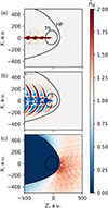 |
Fig. 2. Resulting number density for the interstellar dust particles with sizes of 1000 nm (a), 300 nm (b), and 10 nm (c) in the BV plane. The Sun is at the origin. The solid white lines depict the position of the HP (outer parabolic line) and the TS (inner circular line). |
Medium-sized particles (e.g. 300 nm) penetrate the HP and are strongly affected by the IMF. As noted by Frisch & Slavin (2013), for the stationary magnetic field, the number density of the particles that penetrate the heliosphere is higher in the polar regions of the Sun due to the Lorentz force. The non-stationary IMF causes number density waves in the tail region of the heliosphere (Fig. 2b) because the magnetic field lines and the velocity of the plasma are tangential to the HP, resulting in the electric field normal to the HP. This electric field either pushes particles out or drags them inside the heliosphere, depending on the phase of the solar activity cycle. A cavity forms behind the Sun due to the combined effect of the radiation pressure (also known as β-cone) and the defocusing of the particles near the equatorial plane of the Sun (see e.g. Godenko & Izmodenov 2023a).
Since the electromagnetic force is related to the size of the particle approximately as a−2, large particles are mainly affected by gravity and follow the hyperbolic trajectories. This causes the number density bulge behind the Sun (Landgraf 2000).
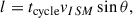
The resulting synthetic mid-infrared images of the heliosphere from different angles between the direction towards the observer and the relative velocity of the Sun and ISM are shown in Fig. 3. Particles that penetrate the heliosphere have a higher emissivity because their temperature is higher, which causes the wavy features in the synthetic intensity maps. The distance between the local intensity maxima corresponds to the solar cycle and the apparent relative velocity of the Sun as
 (6)
(6)
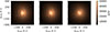 |
Fig. 3. Synthetic intensity maps of the thermal emission of interstellar dust (at wavelength of 50 μm) in the vicinity of the Sun. The angle between the line of sight and the relative velocity vector of the Sun is 90° (left), 60° (middle), and 30° (right). xLOS and yLOS stand for the local coordinates in the projection plane. |
where l is the distance between the intensity maxima, tcycle is the solar cycle period, vISM is the velocity of the Sun relative to the local ISM, and θ is an angle between the line of sight and the direction of the relative velocity.
When the relative velocity vector lies in the projection plane, the distance between local emission maxima is l ≈ 120 a.u. With decreasing θ, the waves are smeared together and become almost indistinguishable at θ ≈ 30°. The faint arc in front of the star is the emission of the ISD particles outside of the HP.
We also calculated intensity maps and the spectral emission distribution (SED) for an observer at 1 parsec using the MRN size distribution, the truncated power-law size distribution (Mathis 1996), and the size distribution and material composition by Hensley & Draine (2023). The changes in the intensity maps are almost indistinguishable, and the effect on the SED is rather quantitative, not qualitative (Fig. 4) because the infrared image is mostly affected by medium-sized particles, for which the size distribution is relatively well constrained. Moreover, PAH or carbonaceous particles are relatively small and therefore stay in the outer shock layer.
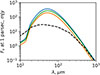 |
Fig. 4. Spectral emission distribution of interstellar dust particles inside the heliosphere for three different size distributions of particles. Classical MRN (green) (Mathis et al. 1977), a truncated power law (blue) (Mathis 1996), and the most recent (orange) (Hensley & Draine 2023). The dashed line indicates the interplanetary dust SED from Poppe et al. (2019). |
An actual image of the Sun would also include the emission of the debris disc, which is located near the ecliptic plane. Poppe et al. (2019) calculated the emission and SED of the modelled debris disc of the Sun. The SED of the interstellar dust exceeds that of the interplanetary dust at wavelengths ≈20..300 μm, with the flux maximum at ≈200 mJy near 50 μm. The relative luminosity of the interstellar dust is LISD/L⊙ ≈ 7 ⋅ 10−7, and in the same order as the luminosity of the interplanetary dust, which suggests a strong effect of the interstellar dust on the infrared excess of the Sun.
4. Conclusions
We performed a Monte Carlo computation of the interstellar dust distribution in the global heliosphere using a numerical kinetic-MHD model of the heliosphere to investigate the effect of the changing IMF on the mid-infrared picture of the Sun. We list the results of our computations below.
-
The medium-sized particle distribution inside the heliosphere is strongly affected by the IMF, which shapes number density waves through the change in the IMF during the solar magnetic activity cycle.
-
These waves are visible in the thermal emission maps in the mid-infrared from different angles, up to ≈30° between the relative velocity and the direction to the observer. The distance between local emission maxima is related to the activity cycle period and apparent motion of the Sun relative to the local ISM.
Using the Sun as an example, we demonstrated overall that infrared images of the astrospheres might be sources of new unique information on the stellar activities.
Acknowledgments
Authors acknowledge support from the Russian Science Foundation grant 25-12-00240. Authors also thank Egor Godenko for providing the dust distribution in the heliosphere.
References
- Alexashov, D. B., Katushkina, O. A., Izmodenov, V. V., & Akaev, P. S. 2016, MNRAS, 458, 2553 [NASA ADS] [CrossRef] [Google Scholar]
- Baalmann, L. R., Janisch, T., Hunziker, S., et al. 2025, A&A, 698, A138 [NASA ADS] [CrossRef] [EDP Sciences] [Google Scholar]
- Baliunas, S. L., Donahue, R. A., Soon, W. H., et al. 1995, ApJ, 438, 269 [Google Scholar]
- Baranov, V. B., Krasnobaev, K. V., & Kulikovskii, A. G. 1970, Akademiia Nauk SSSR Doklady, 194, 41 [NASA ADS] [Google Scholar]
- Bellotti, S., Petit, P., Jeffers, S. V., et al. 2025, A&A, 693, A269 [NASA ADS] [CrossRef] [EDP Sciences] [Google Scholar]
- Bohren, C. F., & Huffman, D. R. 1998, Absorption and Scattering of Light by Small Particles (Wiley-VCH) [Google Scholar]
- Boro Saikia, S., Jeffers, S. V., Morin, J., et al. 2016, A&A, 594, A29 [NASA ADS] [CrossRef] [EDP Sciences] [Google Scholar]
- Cox, N. L. J., Kerschbaum, F., van Marle, A. J., et al. 2012, A&A, 537, A35 [NASA ADS] [CrossRef] [EDP Sciences] [Google Scholar]
- Draine, B. T. 2003, ARA&A, 41, 241 [NASA ADS] [CrossRef] [Google Scholar]
- Drudis, J. M., & Gvaramadze, V. V. 2020, Res. Notes Am. Astron. Soc., 4, 169 [Google Scholar]
- Frisch, P. C., & Slavin, J. D. 2013, Earth Planets Space, 65, 175 [Google Scholar]
- Godenko, E. A., & Izmodenov, V. V. 2023a, Fluid Dyn., 58, 274 [NASA ADS] [CrossRef] [Google Scholar]
- Godenko, E. A., & Izmodenov, V. V. 2023b, Adv. Space Res., 72, 5142 [NASA ADS] [CrossRef] [Google Scholar]
- Godenko, E. A., & Izmodenov, V. V. 2024a, Fluid Dyn., 59, 521 [Google Scholar]
- Godenko, E. A., & Izmodenov, V. V. 2024b, A&A, 687, L4 [NASA ADS] [CrossRef] [EDP Sciences] [Google Scholar]
- Grun, E., Zook, H. A., Baguhl, M., et al. 1993, Nature, 362, 428 [Google Scholar]
- Gvaramadze, V. V. 2020, Res. Notes Am. Astron. Soc., 4, 213 [Google Scholar]
- Hensley, B. S., & Draine, B. T. 2023, ApJ, 948, 55 [Google Scholar]
- Izmodenov, V. V., & Alexashov, D. B. 2015, ApJS, 220, 32 [NASA ADS] [CrossRef] [Google Scholar]
- Izmodenov, V. V., & Alexashov, D. B. 2020, A&A, 633, L12 [NASA ADS] [CrossRef] [EDP Sciences] [Google Scholar]
- Jeffers, S. V., Mengel, M., Moutou, C., et al. 2018, MNRAS, 479, 5266 [NASA ADS] [CrossRef] [Google Scholar]
- Jeffers, S. V., Kiefer, R., & Metcalfe, T. S. 2023, Space Sci. Rev., 219, 54 [CrossRef] [Google Scholar]
- Katushkina, O. A., & Izmodenov, V. V. 2019, MNRAS, 486, 4947 [Google Scholar]
- Kobulnicky, H. A., Chick, W. T., Schurhammer, D. P., et al. 2016, ApJS, 227, 18 [Google Scholar]
- Landgraf, M. 2000, J. Geophys. Res., 105, 10303 [NASA ADS] [CrossRef] [Google Scholar]
- Larkin, C. J. K., Mackey, J., Haworth, T. J., & Sander, A. A. C. 2025, A&A, 700, A60 [NASA ADS] [CrossRef] [EDP Sciences] [Google Scholar]
- Mathis, J. S. 1996, ApJ, 472, 643 [NASA ADS] [CrossRef] [Google Scholar]
- Mathis, J. S., Rumpl, W., & Nordsieck, K. H. 1977, ApJ, 217, 425 [Google Scholar]
- Parker, E. N. 1958, ApJ, 128, 664 [Google Scholar]
- Pogorelov, N. V., Heerikhuisen, J., & Zank, G. P. 2008, ApJ, 675, L41 [NASA ADS] [CrossRef] [Google Scholar]
- Poppe, A. R., Lisse, C. M., Piquette, M., et al. 2019, ApJ, 881, L12 [NASA ADS] [CrossRef] [Google Scholar]
- Russeil, D., Zavagno, A., Bouret, J. C., & Adami, C. 2025, A&A, 698, A64 [NASA ADS] [CrossRef] [EDP Sciences] [Google Scholar]
- Sterken, V. J., Baalmann, L. R., Draine, B. T., et al. 2022, Space Sci. Rev., 218, 71 [CrossRef] [Google Scholar]
- Westphal, A. J., Stroud, R. M., Bechtel, H. A., et al. 2014, Science, 345, 786 [Google Scholar]
- Wilson, O. C. 1978, ApJ, 226, 379 [Google Scholar]
All Figures
|
Fig. 1. Coordinate system used for calculations. The Sun is at the origin, VISM is the relative velocity of the interstellar dust and plasma, BISM is the interstellar magnetic field, and θ is an angle between the direction towards the observer and the velocity of the ISM. |
| In the text | |
|
Fig. 2. Resulting number density for the interstellar dust particles with sizes of 1000 nm (a), 300 nm (b), and 10 nm (c) in the BV plane. The Sun is at the origin. The solid white lines depict the position of the HP (outer parabolic line) and the TS (inner circular line). |
| In the text | |
|
Fig. 3. Synthetic intensity maps of the thermal emission of interstellar dust (at wavelength of 50 μm) in the vicinity of the Sun. The angle between the line of sight and the relative velocity vector of the Sun is 90° (left), 60° (middle), and 30° (right). xLOS and yLOS stand for the local coordinates in the projection plane. |
| In the text | |
|
Fig. 4. Spectral emission distribution of interstellar dust particles inside the heliosphere for three different size distributions of particles. Classical MRN (green) (Mathis et al. 1977), a truncated power law (blue) (Mathis 1996), and the most recent (orange) (Hensley & Draine 2023). The dashed line indicates the interplanetary dust SED from Poppe et al. (2019). |
| In the text | |
Current usage metrics show cumulative count of Article Views (full-text article views including HTML views, PDF and ePub downloads, according to the available data) and Abstracts Views on Vision4Press platform.
Data correspond to usage on the plateform after 2015. The current usage metrics is available 48-96 hours after online publication and is updated daily on week days.
Initial download of the metrics may take a while.