| Issue |
A&A
Volume 705, January 2026
|
|
|---|---|---|
| Article Number | A28 | |
| Number of page(s) | 16 | |
| Section | Extragalactic astronomy | |
| DOI | https://doi.org/10.1051/0004-6361/202453502 | |
| Published online | 24 December 2025 | |
The halo magnetic field of a spiral galaxy at z = 0.414
1
Max-Planck-Institut für Radioastronomie, Auf dem Hügel 69, D-53121 Bonn, Germany
2
Max-Planck-Institut für Astronomie, Königstuhl 17, D-69117 Heidelberg, Germany
3
Thüringer Landessternwarte, Sternwarte 5, D-07778 Tautenburg, Germany
4
Research School of Astronomy & Astrophysics, Australian National University, Canberra, ACT 2611, Australia
5
Department of Astronomy and Astrophysics, University of California Santa Cruz, 1156 High St, Santa Cruz, 95064 CA, USA
6
Dunlap Institute for Astronomy and Astrophysics, University of Toronto, 50 St. George Street, Toronto, ON M5S 3H4, Canada
7
David A. Dunlap Department of Astronomy and Astrophysics, University of Toronto, 50 St. George Street, Toronto, ON M5S 3H4, Canada
★ Corresponding author: This email address is being protected from spambots. You need JavaScript enabled to view it.
Received:
18
December
2024
Accepted:
14
July
2025
Abstract
Aims. Even though magnetic fields play an important role in galaxy evolution, the redshift evolution of galactic-scale magnetic fields is not well constrained observationally. In this paper we provide an observational constraint on the timescale of the mean-field dynamo, and derive the magnetic field in a distant galaxy at z = 0.414.
Methods. We obtained broadband spectro-polarimetric 1−8 GHz Very Large Array observations of the lensing system B1600+434, which is a background quasar gravitationally lensed by a foreground spiral galaxy into two images. We applied rotation measure (RM) synthesis and Stokes QU fitting to derive the RM of the two lensed images, which we used to estimate the lensing galaxy’s magnetic field.
Results. We measured the RM difference between the lensed images and detected Faraday dispersion caused by the magneto-ionic medium of the lensing galaxy at z = 0.414. Assuming that the RM difference is due to the large-scale regular field of the galaxy’s halo, we measured a coherent magnetic field with a strength of 0.2−3.0 μG at 0.7 kpc and 0.01−2.8 μG at 6.2 kpc vertical distance from the disk of the galaxy. We derive an upper limit on the dynamo e-folding time: τdynamo < 2.9 × 10⁸ yr. We find turbulence on scales below 50 pc and a turbulent field strength of 0.2−12.1 μG.
Conclusions. We measured the magnetic field in the halo of a spiral galaxy and find turbulence on scales of < 50 pc. If the RM difference is due to large-scale fields, our result follows the expectation from mean-field dynamo theory and shows that galaxies at z ≃ 0.4 already have magnetic field strengths similar to present-day galaxies. There is one caveat, however: we note the possibility of the turbulent field of the lensing galaxy contributing to the observed RM difference.
Key words: magnetic fields / polarization / methods: observational / galaxies: ISM / galaxies: magnetic fields
© The Authors 2025
 Open Access article, published by EDP Sciences, under the terms of the Creative Commons Attribution License (https://creativecommons.org/licenses/by/4.0), which permits unrestricted use, distribution, and reproduction in any medium, provided the original work is properly cited.
This article is published in open access under the Subscribe to Open model.
Open Access funding provided by Max Planck Society.
1. Introduction
Magnetic fields play an important role in the formation and evolution of galaxies (Beck et al. 2019) as they can affect the gas dynamics (Moon et al. 2023), galactic outflows (Hanasz et al. 2013), the propagation of cosmic rays (Wiener et al. 2013), the star formation rate (SFR, Birnboim et al. 2015; Tabatabaei et al. 2017), and the stellar initial mass function (Rees 1987; Krumholz & Federrath 2019). The evolution of magnetic fields over cosmic time is still not well constrained due to observational challenges.
The evolution of large-scale magnetic fields (> 1 kpc) is described by the mean-field dynamo theory. It can reproduce the magnetic field measurements on scales of several kiloparsecs in nearby galaxies, such as magnetic pitch angle and the strength of the mean magnetic field (e.g., Chamandy et al. 2016; Beck et al. 2019). Dynamo theory describes how kinetic energy is converted into magnetic energy (the amplification of the magnetic field strength) and how the turbulent magnetic field is transformed into a regular (also called coherent) magnetic field. Regular fields have a well-defined direction in the telescope beam, on kiloparsec scales, resulting in a finite average over the beam. On the other hand, turbulent fields on scales of a few hundred parsecs have spatial reversals, and their average over the beam vanishes. Furthermore, turbulent fields can be either isotropic (i.e., random, with the same spatial dispersion in all directions) or anisotropic (with a preferred orientation, but can reverse their direction in the telescope beam)1. The large-scale dynamo, which operates on kiloparsec scales, requires the large-scale differential rotation of the galaxy’s disk. Disks can already form at high redshift, for example at z ∼ 2 − 3 based on observations of ionized gas (Genzel et al. 2006), and at z ≃ 4.4 based on molecular gas (Tsukui & Iguchi 2021). This allows the possibility of large-scale fields on scales of a few kiloparsecs existing in galaxies even at z = 2, as there could be enough time since the formation of the disk (z = 4.4) for the large-scale coherent field to develop (∼2 Gyr, Arshakian et al. 2009). Modeling the dynamo consistently requires that we know the evolution of the physical parameters controlling dynamo action (e.g., angular velocity of galactic rotation, disk size, and gas density); we need to be able to compare the derived magnetic field evolution (Arshakian et al. 2009; Pakmor et al. 2018; Pfrommer et al. 2022) to observations of the regular magnetic field in distant galaxies.
The strength and structure of magnetic fields in local galaxies can be traced by synchrotron emission (see, e.g., Beck et al. 2019). The total synchrotron intensity measures the plane of the sky component of the total (regular and turbulent) magnetic field, and its degree of polarization tells us about the ordered (regular and anisotropic turbulent) magnetic field. However, these techniques have only been used in nearby galaxies, with current redshift limits of z = 0.009 for individual galaxies and z = 0.018 for interacting galaxies (Beck 2013). The primary hurdle is the faint polarized synchrotron emission of galaxies when compared with the sensitivity of current-generation radio facilities. Even with the upcoming Square Kilometre Array (SKA) we can only realistically detect such polarized emission up to z = 0.5 (Beck & Wielebinski 2013). Furthermore, the limited angular resolution causes high redshift galaxies to appear as point sources, making it impossible to study the structure of magnetic fields. Another way to trace the magnetic fields is by using the polarized infrared emission of dust (see, e.g., Lopez-Rodriguez et al. 2022 in nearby galaxies and Geach et al. 2023; Chen et al. 2024; de Roo et al. 2025 in distant galaxies). One limitation of this method is that it traces the ordered magnetic field, i.e., the combination of the regular and the anisotropic turbulent fields, and thus it is unable to provide a constraint on the mean-field dynamo theory; based on dust polarization observations of the disks of nearby galaxies, it appears to originate mostly from anisotropic turbulent fields (Beck et al. 2019). Additionally, for distant galaxies, the limited angular resolution also remains an issue, and can only be studied in the special cases of lensed galaxies (Geach et al. 2023; Chen et al. 2024; de Roo et al. 2025). Thus, it is difficult to obtain for a large sample.
To measure the regular field, Faraday rotation experiments are needed. Only a handful of measurements exist in distant individual galaxies (Kronberg et al. 1992; Wolfe et al. 2011; Mao et al. 2017), along with some statistical detections in intervening galaxies using samples of absorption line quasar systems (Bernet et al. 2008, 2013; Farnes et al. 2014, 2017; Lan & Prochaska 2020; and further discussed by Basu et al. 2018). These results suggest that galaxies up to z = 3 may have comparable magnetic field strengths to local galaxies. Mao et al. (2017) demonstrated a method that can directly measure the coherent magnetic field strength in distant galaxies through observations of a polarized background quasar lensed by a foreground galaxy. By comparing the rotation measure (RM) of the lensed images of the background source, the strength and structure of the magnetic field in the lensing galaxy can be constrained. The polarized light of the background source undergoes Faraday rotation when it passes through the magneto-ionic medium along the line of sight, which causes the polarization angle to change as a function of wavelength, characterized by the RM. The RM ([rad m−2]) is defined as the line-of-sight (l [pc]) integral of the electron density (ne [cm−3]) and the line-of-sight component of the magnetic field (B|| [μG]):
 (1)
(1)
Because of the line-of-sight integral, the observed RM of the lensed images consists of the RM from multiple contributors along the line of sight: the host galaxy of the background quasar (RMqso), the intervening galaxy of interest (RMgal), the intergalactic medium (IGM; RMIGM), and the Milky Way (MW; RMMW). The total observed RM of the polarized light from a quasar at zqso lensed by a galaxy at zgal can be written as
 (2)
(2)
where RMqso and RMgal are rest frame RMs and the (1 + z)2 term is the standard conversion factor to the observer’s frame. As lensing is achromatic (Schneider et al. 1992) and nonpolarizing (Dyer & Shaver 1992), and assuming that the background source RM does not vary on the timescale of the gravitational time-delay, RMqso is the same in both images. The differences in the RM contributions of the IGM (Vernstrom et al. 2019) and the Milky Way (Oppermann et al. 2012; Hutschenreuter et al. 2022) are negligible between sightlines because the angular separation between the lensed images is on the scale of arcseconds or less (for estimates on these for the target in this paper, see Section 3.3). As a result, any difference between the RMs of the images is dominated by the magneto-ionic medium of the lensing galaxy (Narasimha & Chitre 2004; Mao et al. 2017).
For this paper we estimated the magnetic field properties in the lensing system B1600+434, which has the prospect of probing the halo magnetic field strength in a galaxy at an intermediate redshift of z = 0.414. In the top panel of Fig. 1, we show the optical image of the system from Kochanek et al. (1999). This system was discovered by Jackson et al. (1995), who found it to be a two-image lensing system with an image separation of 1.39″. The redshift of the background quasar is z = 1.589 and the lensing galaxy is at z = 0.414 (Fassnacht & Cohen 1998). The lensing galaxy is an edge-on spiral: its axial ratio (a/b, where a and b are the major and minor axis) is 2.4 ± 0.2 and its position angle is 46° ± 3° (Jaunsen & Hjorth 1997), with an inclination of  (Maller et al. 2000). The sightlines of the lensed images go through the halo, one above the disk (image A) and the other below (image B). This system complements the results of the lensing galaxy of B1152+199 from Mao et al. (2017), as the two lensing galaxies are at similar redshifts, but the sightlines of B1152+199, in contrast, probe the disk of its lensing galaxy. These two systems together allow us to investigate the general magnetic field properties of a typical star-forming main sequence galaxy at z ≃ 0.4.
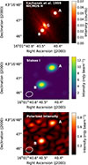 |
Fig. 1. Near Infrared Camera and Multi-Object Spectrometer (NICMOS) H-band image (top) of the lensing system from Kochanek et al. (1999), and the Stokes I (middle) and polarized intensity (PI, bottom) maps from our VLA data. A and B indicate the lensed images of the background quasar, and G shows the lensing galaxy. The lensing galaxy can only be seen in the NICMOS H image, and is too faint to be detected in our VLA images. The Stokes I and PI maps are 16 MHz channel maps at 3.7 GHz. The beam size is shown in the lower left corner. |
This paper is organized as follows. In Section 2 we describe the data reduction of our observations with the Karl G. Jansky Very Large Array (VLA), and in Section 3 we show the results from the RM synthesis and Stokes QU fitting. In Section 4 we estimate the magnetic field strength of the lensing galaxy, investigate how typical the lensing galaxy’s properties are, and discuss the implications of our findings on the large-scale magnetic field amplification mechanism in galaxies. Finally, we present an overview of the typical magnetic fields of galaxies at z ≃ 0.4 and make a comparison to B1152+199 (Mao et al. 2017). We summarize our findings in Section 5. Throughout the paper we use the cosmological parameters derived by Planck Collaboration XIII (2016, Ωm = 0.3089, ΩΛ = 0.6911, H0 = 67.74 km s−1 Mpc−1) when calculating cosmic time and length scales from redshift (Wright 2006).
2. Data analysis
2.1. VLA data and imaging
2.1.1. Original data
We performed broadband spectro-polarimetric observations over 1−8 GHz (L, S, and C band) of the lensing system B1600+434 with the VLA in the A-array configuration. We chose a secondary polarization calibrator, J2202+4216, which is one of the suggested polarization calibrators for the VLA2. However, this source can have moderate time variability, and therefore does not have a standardized model of its polarization angle (PA) and polarization fraction (PF). Thus, in addition to our science observation (from here on the science dataset), we also performed an observation to obtain a model for the polarization properties of J2202+4216 (calibration dataset). The science and calibration datasets were observed on 29 October 2012 and 27 October 2012, respectively. We used the Common Astronomy Software Applications package (CASA, version 5.3.0-143, McMullin et al. 2007; Emonts et al. 2020; CASA Team 2022) and used standard procedures to calibrate the data and to make image cubes of all Stokes parameters.
First, we used the calibration dataset to obtain the polarization information of J2202+4216, which we then utilized to calibrate the science dataset. In the calibration dataset we observed 3C 138 as the flux density and polarization calibrator, and J0319+4130 as the leakage calibrator. For the flux calibration, we used the Perley & Butler (2013a) flux density models; the polarization model for 3C 138 was taken from Perley & Butler (2013b). We generated Stokes I, Q, and U images of J2202+4216 with 16 MHz channel width from 1 to 8 GHz. We used the Clark (1980) deconvolver and Briggs (1995) weighting with a robust parameter of −2. We used the task imfit to fit J2202+4216 on the channel images and to determine its flux density. In Stokes I, we fixed the minor and major axes and the position angles for the fitted Gaussian functions to be the same as the synthesized beam, and we only let the positions and amplitudes change. The errors of the flux densities are given by the root mean square (rms) noise of a source-free region in each image. We fitted the polarization angle and the polarization fraction of J2202+4216 with a polynomial as a function of frequency, and we used this as a polarization model in the science dataset.
For the science dataset, we used 3C 48 as the flux density calibrator, J2202+4216 as the polarization calibrator, J2355+4950 as the leakage calibrator, and J1545+4751 as the phase calibrator. We note that we could not use 3C 48 as a polarization calibrator for the entire dataset as it has low polarization below 4 GHz (⪅3%3), which is why we had to use J2202+4216. For the flux calibration we used the Perley & Butler (2013a) models, and for the polarization calibration we used the model of J2202+4216 that we determined from our calibration dataset. As a quick independent check to see if the calibration was done correctly, we imaged 3C 48 in Stokes I, Q, and U, as this source was not used in the polarization calibration procedure. We found the PA and polarization fraction as a function of frequency to be consistent with those from Perley & Butler (2013b).
We produced images with 16 MHz channel in width (see Stokes I in the middle panel and the polarized intensity in the bottom panel of Fig. 1) and derived the flux density in the same way for our target, B1600+434, in the science dataset, as we did for J2202+4216 in the calibration dataset. However, the lower angular resolution below 1.5 GHz leads to the spatial blending of the two lensed images, and therefore we also fixed the positions of the fitted Gaussian functions in this frequency range, based on their positions between 1.5 and 2 GHz. While this method worked satisfactorily between 1.3 and 1.5 GHz, we were unable to confidently separate the two lensed images and obtain accurate flux densities below 1.3 GHz. We therefore did not include those data in our further analysis.
2.1.2. Follow-up data in L band
To investigate whether the variability of the background source affects the derived RM (see Section 3.3.2) we conducted follow-up observations of B1600+434 using the VLA in L band (1−2 GHz) on 17 February 2021. The flagging, calibration, and imaging essentially followed the steps for the main science dataset, described in Section 2.1.1, and we used 3C 286 as the flux density and polarization calibrator, J1407+2827 as the leakage calibrator, and J1545+4751 as the phase calibrator.
2.2. Properties of the lensing galaxy of B1600+434
To see whether the lensing galaxy is a typical galaxy, i.e., whether it is on the main sequence of galaxies (see, e.g., Noeske et al. 2007; Schreiber et al. 2015; Popesso et al. 2023), we investigated its properties. The lens galaxy of B1600+434 is an edge-on spiral galaxy at z = 0.414. From lens modeling, the total mass (which includes dark matter, stars, gas, and dust) enclosed within the Einstein radius can be determined. The Einstein radius (θE) is half of the image separation (θ). In the case of B1600+434, θ = 1.4″, which means the Einstein radius is 3.85 kpc at the redshift of the lensing galaxy. The enclosed total mass, log(M/M⊙), is estimated to be between 10.97 and 11.11 (Jaunsen & Hjorth 1997; Fassnacht & Cohen 1998; Koopmans et al. 1998). Girelli et al. (2020) found that according to the stellar-to-halo mass relation (derived from combining stellar mass functions from the COSMOS field with a cosmological N-body simulation), a halo with log(M/M⊙)∼11 has a stellar mass of log(M*/M⊙)∼8.5. As the Einstein radius does not enclose the whole galaxy, the galaxy is suspected to have a higher stellar mass than log(M*/M⊙)∼8.5, suggesting that it is a normal size galaxy and not a dwarf.
We fitted the spectral energy distribution with CIGALE (Burgarella et al. 2005; Noll et al. 2009; Boquien et al. 2019) using five optical to near-infrared photometry points (Jaunsen & Hjorth 1997; Jackson et al. 2000) to constrain the galaxy properties. We derived a stellar mass of log(M*/M⊙) = 10.5 ± 0.3 and SFR of 4.1 ± 2.8 M⊙/yr. Even though the SFR has a large uncertainty, this places the galaxy broadly at the main sequence of star-forming galaxies (SFRMS ∼ 6 ± 1 M⊙/yr at z ∼ 0.4 for this stellar mass range, Popesso et al. 2023), suggesting that the galaxy is a normal star-forming galaxy.
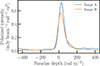 |
Fig. 2. Clean Faraday depth spectra of image A and image B. |
3. Results
3.1. Rotation measure synthesis
To estimate the polarization properties of the lensed images, we performed RM synthesis (Brentjens & de Bruyn 2005) on our target source, using the Python package RM-Tools (Purcell et al. 2020)4. RM synthesis has three main theoretical parameters that determine what we can observe with our observational setup and channel width (Equations 61−63 from Brentjens & de Bruyn 2005):
-
The resolution in Faraday depth space (δϕ) depends on the bandwidth (Δλ2 = λmax2 − λmin2), where λmax = 0.231 m and λmin = 0.037 m, corresponding to 8 GHz and 1.3 GHz, respectively. This results in
 (3)
(3) -
The largest scale in Faraday depth space to which we are sensitive (where sensitivity drops to 50%) depends on the shortest wavelength (λmin) of our observations:
 (4)
(4) -
The maximum observable Faraday depth (||ϕmax||) depends on the channel width (δλ) with more than 50% sensitivity,
 (5)
(5)where the lowest and highest values correspond to the channel widths (chosen to be 16 MHz; see Section 2.1.1), which result in δλ = 1.29 × 10⁻³ m and δλ = 5.63 × 10⁻⁶ m at the lower and higher frequency edge, respectively.
To constrain the residual polarization leakage of our observations, we performed RM synthesis on the leakage calibrators. In the science dataset, we found the apparent polarized flux density (PI =  ) of J2355+4950 to be 0.1 mJy, and its Stokes I flux density to be 1.5 Jy. This corresponds to an upper limit on the residual on-axis polarization leakage of 0.01%. The leakage calibrator J0319+4130 in the calibration dataset has an even lower residual on-axis polarization of 0.003%.
We performed RM synthesis on both lensed images of the target, B1600+434. In Fig. 2, we show the Faraday depth spectra of the lensed images, revealing only a small difference in peak Faraday depth. We calculated the Faraday spectra between −5000 and +5000 rad m−2, with a step of 5 rad m−2, and performed RM clean with a cutoff value of 0.037 mJy (which is three times the theoretical noise level in the spectrum). We find the peaks in the Faraday depth spectra at RMA = +27.4 ± 0.2 rad m−2 and RMB = +21.0 ± 0.4 rad m−2 for the two lensed images. This is calculated by RM-Tools by finding the peak and fitting a parabola to it and its two adjacent points in Faraday depth space (Purcell et al. 2020). The Faraday depth spectra show significant deviation from a single Gaussian-like component; for example, in the case of image B, there is a slight bump toward positive Faraday depth (∼ + 150 rad m−2), which could indicate a Faraday complex source.
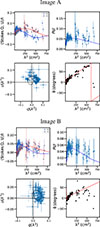 |
Fig. 3. QU fitting results for images A (top panels) and B (bottom panels). Top row of each panel: Fractional Stokes parameters (q = Q/I, u = U/I), and fractional polarized intensity (PI/I) as a function of λ2. Bottom row of each panel: u as a function of q, and polarization angle as a function of λ2. The fitted models are overlaid as dashed lines. |
3.2. Stokes QU fitting
Stokes QU fitting (see, e.g., Farnsworth et al. 2011; O’Sullivan et al. 2012; Ma et al. 2019) is better at disentangling multiple polarized components than RM synthesis, as Farnsworth et al. (2011) previously showed. Thus, we used this method, and fitted the fractional Stokes parameters q = Q/I and u = U/I as a function of frequency for both of the lensed images.
We fitted several models to the Stokes q and u of the lensed images independently, also considering internal and external depolarization (Sokoloff et al. 1998). One scenario is the Faraday thin model, where a synchrotron emitting source is behind a Faraday rotating screen with a homogeneous magnetic field and thermal electron density (i.e., the turbulence is on larger scales than the projected size of the background source). Another type is the Burn (1966) slab model with a foreground rotating screen, where the synchrotron emitting volume is also Faraday rotating. There is also the external dispersion model, where we have a turbulent Faraday screen in the foreground (i.e., the turbulence is on smaller scales than the projected size of the background source) that causes depolarization effects. Finally, internal dispersion with the foreground, where the synchrotron emitting volume is also Faraday rotating and has a turbulent magnetic field. In the case of the Faraday thin, Burn slab, external dispersion, and internal dispersion models, we tried both single and double models, where there are respectively one and two spatially unresolved synchrotron emitting sources in the plane of the sky, i.e., polarized components (for more details on the specific models, see, e.g., Ma et al. 2019).
We chose the best model to be the one that resulted in the lowest Bayesian information criterion (BIC) value. A difference of more than 10 in the BIC value indicates a strong preference for a model with the lower BIC (Schnitzeler 2018). The best model was one with a background source with two spatially unresolved polarized components, and two external Faraday rotating screens that have turbulence on scales smaller than the projected size of the lensed quasar. The σRM that can be measured through QU fitting arises from turbulence on these small scales. However, we note that the screens can also have turbulence on larger scales, assuming a Kolmogorov-type spectrum (Kolmogorov 1991) for the turbulent energy density with different strengths at different scales. This model was the best for both lensed images (with a BIC ∼ 40 lower than the next best model, double Faraday thin), shown in Fig. 3. The complex polarization as a function of λ2 is given by
 (6)
(6)
where λ is the wavelength, PF1 and PF2 are the intrinsic polarization fractions, PA1 and PA2 are the intrinsic polarization angles, RM1 and RM2 are the RM values, and σRM, 1 and σRM, 2 represent the Faraday dispersions of the two components. In this model, we also assume that the polarized components have the same spectral index. The best-fit parameters are listed in Table 1. The presence of two polarization components is consistent with observations from the Very Large Baseline Array (VLBA) that show the substructure of the background source in Stokes I, with two subarcsecond scale spatial components in both the lensed images (Biggs 2021), which are spatially unresolved in our VLA observations.
Stokes QU fitting results of the two polarized components of B1600+434 for the two lensed images.
In the rest of the paper, we refer to the polarized component with the larger PF as the main polarized component and the other as the secondary. The PA and PF values of the two polarized components are consistent between images A and B, suggesting that we are observing the same background source and its components in both the lensed images. We find a small difference in the RM (RMA, 1 vs. RMB, 1, and RMA, 2 vs. RMB, 2) and σRM (σRM, A, 1 vs. σRM, B, 1, and σRM, A, 2 vs. σRM, B, 2) of both components between the two images. This is most likely caused by the differences in the lensing galaxy’s magneto-ionic medium in the two regions probed by the lensed images. The RM of both components is larger in image A, and σRM is slightly larger in image B (although for the secondary component, the values agree within the errors).
We tried to connect the polarized components to their possible physical sources. Active galactic nuclei (AGN) usually have larger |RM|s compared to the jet (Hovatta et al. 2019). Thus, the main polarized component most likely corresponds to the jet with a lower |RM| ∼20 rad m−2, and the secondary component to the emission near the core of the AGN with a high |RM| ∼300 rad m−2. However, it is worth noting that as the observed RM is a sum of the different components along the line of sight, a contribution of ∼ − 150 rad m−2 or lower would change which component has a higher |RM|. We do not expect such a large contribution from the MW and the IGM (see Section 3.3.1). However, the lensing galaxy might contribute such a large RM in the case of a strong magnetic field, a larger free electron density, or a combination of the two. We note that the emission from the AGN core would have a flatter spectrum than that of the jet. This would mean that the main (jet) component is mainly seen at low frequencies and the secondary (core) component at high frequencies. The large σRM, 2 values might be due to this effect (in contrast to being caused by a depolarizing medium), as it would result in a fit where the secondary component is suppressed at low frequency. Nevertheless, this would not affect the main component’s RM difference between the lensed images, and in the rest of the paper, we do not use σRM, 2, so this would not affect the results of our paper.
We note that the secondary component is not seen in the clean FDF at the same RM that is derived from Stokes QU fitting (Fig. 2). This is not that surprising as, for example, Farnsworth et al. (2011) has shown that Stokes QU fitting is better at disentangling multiple RM components than RM synthesis.
3.3. RM difference and possible causes
After deriving the observed RM of the two quasar images with QU fitting, we get an RM difference of 8 ± 2 rad m−2 and 71 ± 94 rad m−2 from the two components. These results are consistent within the errors and also with those obtained using RM synthesis (see Section 3.1, Fig. 2). In the rest of the paper we use the result from the Stokes QU fitting, and due to the large uncertainty of the RM difference from the secondary polarized component, we only consider the RM difference of the main component. RM synthesis is more sensitive to the main component, and the secondary component is only captured by QU fitting. In this section, we investigate whether the RM difference can be caused by something else apart from the lensing galaxy’s magneto-ionic medium.
3.3.1. Contributions from the Milky Way and the intergalactic medium
According to the Hutschenreuter et al. (2022) Galactic RM map, the Milky Way’s contribution is 16.6 rad m−2 along the line of sight toward B1600+434, but the variation in a 10 arcmin radius around the source is only 1.4 rad m−2, implying that the variation on smaller scales could be even lower. However, we note that this reflects only RM uncertainty, not the RM dispersion from the Milky Way. Extrapolated from the north Galactic pole’s RM structure-function (Stil et al. 2011), we expect the Galactic RM fluctuation to be ≲1.8 rad m−2 on arcsec scales. For the case of the IGM contribution, Vernstrom et al. (2019) calculated the RM difference between pairs of sources that could be attributed to the IGM and found it decreases with angular separation, becoming < 1 rad m−2 on the order of arcseconds. These estimates are insufficient to explain the observed RM difference.
3.3.2. Effects of time variability of the background source
If there is a time variation in the RM of the background source itself, it can lead to a contribution to the observed RM difference. This is due to the combined effect of the time variability and the time delay of the lensing system. To investigate if this can indeed be the case, we conducted follow-up observations of B1600+434 using the VLA in L band (1−2 GHz), as described in Section 2.1.2.
Biggs (2021) showed that B1600+434 has a time delay of 42.3 ± 2.1 days in radio (51 ± 4 days in optical, Burud et al. 2000) between the two lensed images, and that the background source also exhibits polarization (PI, PA, and PF) variability on similar timescales. As a combined effect of time delay and time variability of the RM of the lensed quasar, the observed RM difference could also change. However, if the RM difference is mainly caused by the magneto-ionic medium of the lensing galaxy (and the properties of the galaxy’s magnetic field do not vary on short timescales), the RM difference should remain constant in time. By monitoring the lensing system in polarization, we can determine the RM variability of the background source, and decide whether the RM difference is caused by the galaxy.
We applied Stokes QU-fitting to the new observations, and we compared the results to the QU fitting of only L band (1.3−2 GHz) of our earlier observations (see Table 2). In Fig. 4 we show the L band (1.3−2 GHz) of our earlier data and our new data, overplotted on our QU fitting model derived from the full frequency range (1.3−8 GHz) of the earlier data. The data points show broad agreement. We calculated the residuals between the two datasets (qold − qnew, uold − unew) separately for image A and B. While these are close to 0, they show a slight variation between the two dates. We also calculated the reduced χ2 of the datasets with respect to the QU model: Q and U for image B have a χ2 lower than 2 for both the original and the follow-up data. However, Q and U for image A in the follow-up data have a χ2 of 4 and 7.5, respectively.
QU fitting result of the two images of B1600+434 in L band (original and new data).
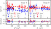 |
Fig. 4. Comparison of our original and our follow-up data in L band. The top row shows Stokes Q/I (blue) and Stokes U/I (red) of our earlier data (empty circles) and our new data (filled circles) as a function of λ2 for image A (left) and image B (right). We also plot the QU fitting model (dashed lines) derived from the full frequency range of the earlier data. The bottom row shows the residual between the two datasets (qold − qnew, uold − unew). |
We chose the model with the lowest BIC as the best-fit model for the L-band-only observations (both original and follow-up): the single Faraday thin model for image A and the single external dispersion model for image B. As the L-band best-fit models are comprised of only one single polarized component, we concluded that we could not observe one of the polarized components found in the main science data. Based on the similarities of the polarization properties of the two lensed images in the L-band-only data to the main polarized components in the full frequency range data, we argue that we found the main polarized component, but we could not observe the secondary component. This is supported by how the secondary component most likely could only be observed with higher frequency data due to its large σRM (or due to its flat spectrum). Even though the observations were taken nine years apart, the polarization properties of the lensed images do not show significant variation. We conclude that the RM of the main polarized component has not changed significantly over time (i.e., it is consistent within the errors), and likewise for the RM difference. This suggests that the RM difference between the images reflects the magneto-ionic medium of the foreground galaxy (i.e., there is no significant contribution by the RM time variability of the background source). However, we note that our follow-up observations have higher uncertainties since we only used a narrower frequency range, which reduces the precision in Faraday space.
3.3.3. Gravitational lensing
Gravitational lensing only introduces additional changes in the polarization angle in the case of a rotating or nonspherical lens. This effect is less than 0.1° if the image is r = 100 m away from the lens (Dyer & Shaver 1992), where m is the geometrized mass (in geometrized unit system). In the case of a galaxy with a stellar mass of log(M*/M⊙) = 12, m is 0.05 pc, and r = 5 pc, which is significantly less than the distance of the lensed images from the lensing galaxy (0.7 and 6.2 kpc). This means we do not expect a change in the polarization angle between the lensed images of the background quasar due to gravitational lensing.
A change in the polarization angle can also be due to birefringence caused by axion-like particles (Basu et al. 2021). However, this effect is achromatic, and thus does not cause a difference in RM.
4. Discussion
4.1. The rest-frame RM difference
After excluding the possibility of other causes in Section 3.3, we proceeded with attributing the RM difference between the lensed images to the magneto-ionic medium of the lensing galaxy. To correct for the redshift dilution, we converted the observed RM (RMobs) of the two quasar images (RMA, obs = 24 ± 1 rad m−2, RMB, obs = 16 ± 2 rad m−2) to rest frame RM (ΔRMrf):
 (7)
(7)
Here zgal = 0.414 is the redshift of the lensing galaxy. The rest-frame RM difference is related to the electron column density (Ne = ∫nedl) and the line-of-sight magnetic field component (B||) as
 (8)
(8)
where the quantities with subscripts A and B correspond to the positions probed by sightlines A and B, respectively. Equation (8) assumes that B|| is constant along the LOS, the path lengths are the same in both sightlines, and the magnetic field and the electron density are uncorrelated. We derive ΔRMrf = 16 ± 4 rad m−2.
In the following, we describe how we investigated whether the small-scale or large-scale field of the lensing galaxy is responsible for the RM difference. For both cases, we needed to first make assumptions on the electron density of the galaxy. The ranges of parameters we used in our calculations are listed in Table C.1.
4.2. Assumptions on electron density
4.2.1. General assumptions
This lensing system was observed with the Chandra X-ray Observatory, from which Dai & Kochanek (2005) derived the differential hydrogen column density based on X-ray absorption (Δ NH = NH, B − NH, A ≃ 3 ⋅ 1021 cm−2). This can be converted into differential electron column density (Δ Ne) by assuming an ionization fraction (fion) lying in a wide range over 5 − 50%; we get Δ Ne = Ne, B − Ne, A = 48.6 − 486.1 pc cm−3. The advantage of this method is that we do not need to assume a path length through the lensing galaxy. This can be directly used in a constant (with distance from the galaxy’s plane) and antisymmetric magnetic field geometry model (see Section 4.4, item 2) to get a B field strength estimate as we only need the ΔNe. However, this assumption is insufficient for other magnetic field geometry models (see Section 4.4, items 3–6) as instead of ΔNe, we need the sum of the electron column densities. Thus, for these models we needed to make another assumption about the electron column density of sightline A. We assumed a wide range of 1 − 100 pc cm−3 for Ne, A, which corresponds to ne = 10−4 − 10−2 cm−3 on average in a 10 kpc sightline. This ranges from approximately 0.5 to 50 times of the MW value at a vertical distance of hA = 6.2 kpc from the midplane of the galaxy (see Section 4.2.2). This results in Ne, B = Ne, A + Δ Ne = 49.6 − 586.1 pc cm−3, and Ne, A + Ne, B = 50.6 − 686.1 pc cm−3. For all the assumed values above, we considered the wide range for parameters fion and Ne, A, to take into account the possibility that high redshift galaxies have different properties than local ones.
4.2.2. Electron density in Milky Way-like galaxies
We also investigated the scenario where we assume Milky Way-like properties for the lensing galaxy (based on our findings in Section 2.2). We estimated the electron column densities by using the electron density profile derived by Ocker et al. (2020) for the Milky Way halo:
 (9)
(9)
Here n0 = 0.015 ± 0.001 cm−3,  kpc, and h is the vertical distance from the Galactic midplane. If we assume the galaxy is completely edge-on, and we calculate with an integral path length of 10 kpc through the halo (see, e.g., Badole et al. 2022), we derive electron column densities of Ne, A = 2 − 4 pc cm−3 and Ne, B = 92 − 100 pc cm−3 at a distance from the plane of the galaxy at hA = 6.2 kpc (image A) and hB = | − 0.7| kpc (image B), respectively. This gives us a differential electron column density Δ Ne = 88 − 98 pc cm−3, which is consistent with using fion = 9 − 10% to calculate Δ Ne from Δ NH. This in turn is in agreement with the ionization fraction of the Galactic interstellar medium (10
 %, He et al. 2013 derived from the dispersion measure and X-ray column density of radio pulsars). The sum of the electron column densities is Ne, A + Ne, B = 94 − 104 pc cm−3.
Our calculations based on Ocker et al. (2020) suggest that Ne, A is more likely to be much less than 100 pc cm−3, unless ne is an order of magnitude higher in galaxy halos at z ∼ 0.4 compared to the Milky Way, in contrast to our general assumptions. Based on spectral line observations of high redshift galaxies (Davies et al. 2021; Isobe et al. 2023), ne could be twice as large in galaxies at z ≃ 0.4 compared to z = 0. This would result in Ne, A = 4 − 8 pc cm−3 and Ne, B = 183 − 200 pc cm−3, and corresponds to an ionization fraction of 18−20%.
The ranges of electron density from the general assumptions in Section 4.2.1 overlap with these values, but have a wider range; thus, we decided to calculate the magnetic field properties with the widest (full parameter range) and narrowest (MW-like parameters) range of parameters.
4.3. Turbulent magnetic field
We detected differential Faraday dispersion, which is due to the amount of turbulence in the lensing galaxy being different in the two sightlines on scales smaller than the projected size of the background source. The differential Faraday dispersion is defined as
 (10)
(10)
From ΔσRM, rf, we can derive an estimate on the small-scale random field (following Mao et al. 2017, and based on Beck 2015), on scales below ∼50 pc5:
 (11)
(11)
where f = 0.02 − 0.14 is the filling factor and N = 10 000 is the number of turbulent cells in the sightline (in the case of l1 = 10 pc cells through a L = 10 kpc sightline). Using MW-like Ne estimates (see Section 4.2), we derive Br ∼1.4−6.9 μG; instead, when considering the full parameter range Br can vary between 0.2 and 12.1 μG. We note that apart from fion and Ne, A, the derived strengths also depend strongly on the assumptions of N and f.
Assuming that the magnetic energy power spectrum is described by a power law, with a slope similar to Kolmogorov turbulence, we can estimate magnetic field strengths on larger scales by extrapolating the strength measured on < 50 pc scales. Thus, we investigate whether turbulent fields can cause the RM difference we see between the two lensed images. For this, we extrapolated the turbulent magnetic field and σRM to scales of l2 = 1000 pc (outer scale of turbulence in the halo of M51, Mao et al. 2015), which is detailed in Appendix A. We assume Kolmogorov spectrum for the turbulence, and we include an additional factor because we are dealing with turbulence in the halo and not in the disk. We derive σRM = 41 ± 11 rad m−2 on scales of 1000 pc, in the rest frame. The parameters that can affect our derived value significantly (i.e., by a factor of 2 if changed by a factor of 2) are the assumed ratio of the halo density to disk density, and the cell size of the turbulence l1 and l2.
The derived σRM on kiloparsec scale is of a similar magnitude to the RM difference between the images, which indicates that the turbulent field is a possible contributor to the measured RM difference. We note that extrapolating σRM to kiloparsec scales heavily depends on the assumed ISM properties. Thus, we also note that the possibility of the turbulent field contributing to the RM difference is a caveat of our method, which can only be completely excluded by joint analysis of more lensing systems (see Section 5).
Derived magnetic field strengths for different magnetic field geometry models.
4.4. Large-scale magnetic field geometries and strengths
4.4.1. General assumptions
In this section we assume that the regular field is responsible for the RM difference between the two lensed images. We derive the magnetic field strength of the lensing galaxy using simplified magnetic field geometry models (listed in Appendix B), ranging from simple constant fields to fields that scale with distance from the galaxy’s plane.
An additional important parameter needed to derive the large-scale regular field strength is the galaxy’s inclination, and (in some of our models) the distance of the lensed images from the midplane. Maller et al. (2000) derived an inclination (i) of  by fitting elliptical isophotes to a Hubble Space Telescope (HST) image of the galaxy. We consider image A to be above the disk with a vertical distance from the midplane (h = 0 kpc) of hA = +6.2 kpc and image B to be below the disk with a vertical distance from the midplane of hB = −0.7 kpc.
The halo field is most likely dominated by poloidal fields, which are best approximated by vertical magnetic fields (i.e., fields perpendicular to the galaxy’s disk) in the inner halo (i.e., at small radii). In this case, the line-of-sight magnetic field component is given by
 (12)
(12)
In summary, we find that if we use models that only assume a vertical field, the magnetic field strength B0 is between 0.2 and 4.1 μG. We show the derived magnetic field strengths at position A and position B in Table 3.
However, it is possible that instead of a poloidal field, there is a dominating toroidal field in the halo. If there is a large-scale dynamo in the galaxy, a toroidal magnetic field will be produced in the disk, which can also be present in the halo due to advection from galactic winds (see, e.g., Krause 2019; Myserlis & Contopoulos 2021). In this case, the RM we see could be mainly due to the toroidal field. Then, the line-of-sight component is given by
 (13)
(13)
where Bt is the strength of the toroidal magnetic field, which we assume to be constant. We derive a field strength between 0.04 to 0.4 μG, lower than the strength resulting from assuming a poloidal field in most cases.
We obtained such a wide range of magnetic field strength values because of the wide range of values for the parameters fion and Ne, A. In Appendices C and D, we explore in detail how each parameter and the choice of the magnetic field geometry model affect the results. In summary, the assumed ionization fraction and the inclination of the galaxy affect the derived magnetic field strengths the most, by a factor of ∼10 and ∼5, respectively. In the case of the position probed by image A, at 6.2 kpc from the midplane of the galaxy, the effect of the scale height is also significant (a factor of ∼10).
We find that all models give similar ranges of magnetic field strength, apart from the toroidal model, which results in low field strengths. However, we cannot rule out any of the models above based on our data, as all of them give reasonable results compared to nearby galaxies and the Milky Way (see Section 4.5).
We note that the sightlines of the lensed images might go through different heights from the plane of the galaxy, compared to the apparent distance, due to the galaxy’s finite inclination. This causes them to go through regions with different magnetic field strengths, proportional to the height from the galaxy’s plane. To estimate the effect of this, we calculated the possible heights on a 10 kpc long sightline (hA = 5.5 to 7 kpc and hB = 0.02 to 1.4), and found the inferred average magnetic field strengths would change by 30−40%.
4.4.2. Large-scale magnetic field strength in the case of Milky Way-like properties
Here we investigate our results for a restricted range of parameters corresponding to MW-like galaxies and electron column densities (ΔNe = 68 − 136 pc cm−3) calculated in Section 4.2 based on the ne profile from Ocker et al. (2020), and assuming a scale height of Hhalo = 2 − 8 kpc for the exponential magnetic field geometry (Beck et al. 2019). We investigated the different geometry models for this parameter case and list the results in Table 3. The exponential model is the most realistic model based on what we see in nearby galaxies; for example, the synchrotron emission shows exponential dependence with distance from the plane, which is also indicative of the magnetic field (see, e.g., Beck 2015; Krause et al. 2018). This results in an absolute vertical magnetic field strength of 1.2−1.8 μG at 0.7 kpc from the plane of the disk (BB) and 0.1−0.9 μG at 6.2 kpc (BA).
4.4.3. Implications of the field amplification mechanism in the lensing galaxy of B1600+434
The mean-field galactic dynamo has a theoretical amplification timescale (e-folding time) of ∼2.5 × 10⁸ yr (Arshakian et al. 2009), for a disk galaxy with an average angular velocity of Ω = 20 km s−1 kpc−1. This timescale describes the time needed to amplify a regular field that is spatially ordered on the scale of a few kiloparsecs. However, the time needed for a large-scale field to be ordered on the scale of the entire galaxy disk (ordering timescale, tens of kiloparsecs) without reversals is only a few times shorter than the lifetime of a galaxy (i.e., one order of magnitude larger, Arshakian et al. 2009).
Present-day magnetic field strengths on the order of μG are expected from the mean-field dynamo theory (Ruzmaikin et al. 1988). We find that the large-scale magnetic field has already built up to present-day magnitude at z = 0.414 (see Section 4.5). The measured magnetic field strength can constrain the amplification timescale of the large-scale coherent magnetic field of galaxies. To derive the e-folding time, we use the following equation (similar to Mao et al. 2017):
![Mathematical equation: $$ \begin{aligned} \tau _{\rm dynamo}\,[\mathrm{Gyr}] = \frac{\Delta t}{\ln (B_{\mathrm{disk}, z = 0.414}/B_{\rm seed})}\cdot \end{aligned} $$](/articles/aa/full_html/2026/01/aa53502-24/aa53502-24-eq19.gif) (14)
(14)
Here Bseed is the seed magnetic field of the mean-field dynamo and Δt = 5.97 Gyr is the time that passed between when the disk settled into equilibrium (z = 2, e.g., Genzel et al. 2006) and the redshift of the lensing galaxy (z = 0.414). Furthermore, we assume that Bhalo = 0.4 Bdisk (Beck et al. 2019)6, where Bdisk, z = 0.414 is the disk field strength at z = 0.414. While this relation was derived for the equipartition magnetic field strength, we argue that it is also true for the regular field, based on observations of M 51 (Shneider et al. 2014, who derived a ratio of 0.3). We take the lowest magnetic field strength value we derived in the MW-like parameter case, so Bhalo = 0.1 μG. We also assume that the magnetic field has already saturated, at the latest, at z = 0.414 (as the derived strengths are consistent with nearby galaxies; see Section 4.5).
There are multiple seed field origin scenarios, mainly divided into primordial fields generated in the early Universe and fields generated during galaxy formation (Subramanian 2019; Beck et al. 2019). The former can be estimated by measurements of cosmic voids and cosmic web filaments. Following the assumption in Mao et al. (2017), Bseed would be ≥3 × 10⁻¹⁶ G (Neronov & Vovk 2010, based on cosmic voids). Using this value, we derive an upper limit on the dynamo e-folding time, τdynamo < 2.9 × 10⁸ yr, which is consistent with the theoretical value (Arshakian et al. 2009). If Bseed is higher, τdynamo will be higher as well: ∼7 − 8 × 10⁸ yr for 0.04 − 0.11 nG (Carretti et al. 2023, from cosmic filaments). However, if Bseed is significantly lower (e.g., 10−21 from Biermann battery origin, Subramanian 2019), it would result in τdynamo < 1.8 × 10⁸ yr, which is lower than the theoretical amplification timescale (Arshakian et al. 2009). In the case of a seed field from the small-scale dynamo, the field strength could be of μG strength, which would result in a much longer possible e-folding time. For example, if we assume a ∼0.1 μG seed field, we derive τdynamo < 6.5 × 10⁹ yr. We note that the apparent relation of a smaller Bseed leading to a better constraint of τdynamo is mainly due to the fact that we assumed the same Δt for all Bseed values for simplicity. This means assuming the properties of the turbulence and turbulence driver remains the same for difference seed fields. However, it is possible that these properties are different. For example, in the case of larger Bseed, the turbulence could be stronger, leading to a quicker amplification of the field (smaller Δt), and eventually resulting in a smaller τdynamo.
These values are upper limits for the e-folding time as the field could have been amplified more quickly than the time between the disk settling into equilibrium and the time when we observed it. The e-folding time could be higher if the disk settled earlier (e.g., τdynamo < 3.8 × 10⁸ yr, if settled at z = 4.4, Tsukui & Iguchi 2021).
We note that conservation of magnetic helicity provides a lower limit of 1.6 on the ratio of random and coherent fields in mean-field dynamos (Shukurov 2007; Mao et al. 2017). Our results at 6.2 kpc are consistent with this; as in the case of MW properties, we derive a ratio of ∼1.6−70. However, the same ratio at 0.7 kpc is ∼0.8−6. This suggests that higher values of turbulent fields are more likely to be true (e.g., in the case of a filling factor of > 0.09, or a turbulent cell size of < 10 pc), or that the lower end of the derived regular field strengths are more likely (e.g., higher fion).
4.5. Comparison to the halo field of nearby galaxies and the Milky Way
In this section, we compare our derived field strengths at z = 0.414, to those of the Milky Way and nearby (present-day) galaxies. The Continuum Halos in Nearby Galaxies – an EVLA Survey (CHANG-ES; Irwin et al. 2012, 2019) has conducted observations of nearby edge-on galaxies and derived their magnetic field properties. We list a few of their results below. The first observational evidence of regular magnetic fields in the halo of nearby galaxies was measured by Mora-Partiarroyo et al. (2019). They found a magnetic field in NGC 4631, which is coherent over 2 kpc in height, and reverses on a scale of 2 kpc along the major axis. The halo field is about 4 μG in strength, lower than its 9 μG disk field, which is similar to what we see when we compare our result to another galaxy’s disk field at z = 0.4 (see Section 4.7). Krause (2019) found 5−10 μG total magnetic field strength in the halos of CHANG-ES galaxies. To compare, we estimate the total magnetic field strength from our results,  G. This is lower than Krause (2019), but the difference could be partly from the contribution of the anisotropic turbulent field, which we neglect in the equation above.
The vertical magnetic field of the Milky Way halo was measured to be −0.14 μG (Taylor et al. 2009) or consistent with 0 μG (Mao et al. 2010) for h > 0 (in the northern Galactic hemisphere), and +0.30 μG for h < 0 (in the southern Galactic hemisphere) by exploiting the Faraday rotation of extragalactic radio sources (Taylor et al. 2009; Mao et al. 2010). Mao et al. (2012) assumed that there is a constant, coherent azimuthal halo magnetic field parallel to the Galactic plane, but with different strengths below and above the disk. They calculated a magnetic field strength of 7 μG below the Galaxy’s plane and 2 μG above it (from 0.8 to 2 kpc).
The ranges of these B field strengths are consistent with our result of 0.2−4.1 μG (see Sect. 4.4). However, we cannot implement models with more free parameters because we only have one ΔRM available for the lensing galaxy of B1600+434. This is why we assume that only the direction of the magnetic field can change below and above the disk, not its strength.
4.6. Comparison to cosmological MHD simulations
We selected star-forming galaxies at z = 0.4 from the TNG50 simulation of the IllustrisTNG project (Pillepich et al. 2019; Nelson et al. 2019), and derived their vertical magnetic field strength profiles from their edge-on magnetic field maps (calculated by integrating through 20−40 kpc depending on the size of a given galaxy). We find that the vertical magnetic field strength is 0.55 μG at 0.7 kpc and 0.2 μG at 6.2 kpc from the midplane. This is consistent with the lower bounds on magnetic field strengths we estimated from our observations. We note that this comparison between the derived large-scale coherent field strengths from our observations and the magnetic field strengths in the simulation is comparing similar quantities, as TNG50 mainly has a large-scale field and has weaker random magnetic fields compared to observations. This is due to the fact that the simulation does not contain all sources of turbulence on small scales that could amplify the turbulent field. The reason behind the low large-scale field strengths could be similarly due to the limited spatial resolution of the simulation (i.e., missing sources of turbulence), and thus does not completely model the mean-field dynamo seeded by random fields (see discussion in, e.g., Kovacs et al. 2024, Section 3.3.4).
This is similar to the missing small-scale turbulence leading to lower magnetic field strengths in the Auriga simulations (Pakmor et al. 2017, 2018) compared to observations. Their vertical magnetic field strength profiles show stronger magnetic field strengths than our results from TNG50, with ∼2 μG at h = 6 kpc and ∼3.5 μG at h = 0.7 kpc. These are consistent with our results considering the full parameter range, but we derive a ∼50% lower value of B at h = 0.7 kpc with MW-like parameters.
4.7. Typical magnetic fields at z ≃ 0.4
Mao et al. (2017) used the same method as we did for the lensing system B1152+199, with a lensing spiral galaxy at z = 0.439, where the sightlines of the lensed quasar images pass through the disk of the galaxy. They detected a coherent magnetic field with field strengths between 4 and 16 μG, and found that the scenario of axisymmetric fields in the disk is favored over the presence of bisymmetric fields. Their results are consistent with the dynamo model because that model predicts that the axisymmetric mode is strongest in the disk (Mao et al. 2017; Shukurov 2005; Arshakian et al. 2009).
The sightlines of B1600+434, on the other hand, pass through the halo of the lensing galaxy, providing information on halo magnetic fields. Assuming that both galaxies are typical spirals at z ≃ 0.4, we can draw an overall view of galactic magnetic fields at that redshift, including the halo and the disk. We find that the halo B field strength in the case of the lensing galaxy of B1600+434 being a Milky Way-like galaxy (0.9−2.5 μG) is lower by a factor of 1.6−19 compared to the disk field (4−17 μG) in the lensing galaxy of B1152+199 (Mao et al. 2017). In most cases, the halo magnetic field strength is also lower than that in the disk when we consider the full parameter range (0.2−4.1 μG) for the former. This is also in agreement with dynamo theory.
5. Conclusions and outlook
We performed broadband VLA radio polarization observations of the gravitational lensing system B1600+434. We detected RM difference between the lensed images (ΔRMrf = 16 ± 4 rad m−2) and differential Faraday dispersion (ΔσRM, rf = 19 ± 5 rad m−2), from which we infer the large-scale and turbulent magnetic field strength in the halo of a spiral galaxy at z = 0.414.
If the RM difference between the lensed images is caused by the regular field, assuming Milky Way-like galaxy properties and an exponential magnetic field model, we find the vertical magnetic field strength to be 1.2−1.8 μG at a vertical distance of 0.7 kpc from the plane of the galaxy and 0.1−0.9 μG at 6.2 kpc. With broader parameter ranges and different geometry models, we find values of 0.01−2.8 μG at 0.7 kpc and 0.2−3 μG at 6.2 kpc. The strength of the halo field is comparable to halo fields measured in nearby galaxies (Beck 2015; Beck & Wielebinski 2013, CHANG-ES Irwin et al. 2012) and the Milky Way (Taylor et al. 2009; Mao et al. 2010, 2012). We note that in contrast to most magnetic field measurements of nearby galaxies, which are based on the equipartition assumption7, our measurements are independent and not based on that assumption, but still show consistent results. This could mean that the mechanism generating the large-scale magnetic field has already built up the regular field strength to what we see in present-day galaxies at a redshift of 0.414. We detected differential Faraday dispersion (ΔσRM) between the lensed images, which is indicative of turbulent magnetic fields on scales lower than 50 pc in the halo of the lensing galaxy. The corresponding field strengths are 1.4−6.9 μG considering MW-like galaxy properties, and 0.2−12.1 μG considering a wider range. We note that there is a possibility that part of the differential RM is caused by the turbulent field.
We put our results in context with the dynamo theory. We derive a dynamo e-folding time of < 2.9 × 10⁸ yr, consistent with theory (Arshakian et al. 2009). Dynamo theory predicts that the small-scale turbulent field is stronger than the large-scale field, and that the disk field is stronger than the halo field. We find both of these criteria are fulfilled by our results as the small-scale turbulent magnetic field (1.4−6.9 μG) is stronger in most cases than the large-scale coherent field (1.2−1.8 μG), and the halo magnetic field in the lensing galaxy is weaker compared to the disk field of a similar galaxy at z ≃ 0.4 (Mao et al. 2017).
We demonstrated that many parameters are important for the accurate derivation of the magnetic field strength in lensing galaxies, and for excluding the possibility of turbulent fields in the lensing galaxy causing the RM difference. These could be overcome if we have a large enough sample; for example, the SKA is expected to observe 105 new lensing systems (McKean et al. 2015), which will significantly increase the number of suitable systems for magnetic field studies.
We note the importance of higher frequency data (e.g., S and C band) in detecting the Faraday dispersion caused by the lensing galaxy. As we show in Section 3.3, observing only in L band can miss polarized emission over broad Faraday depth components (the inability to measure σRM). The presence of a polarized component with statistically significant σRM can help us quantify how much turbulent fields contribute to the measured RM difference between sightlines. However, the estimation depends on a few elusive ISM turbulence parameters: the characteristic size of the turbulence that caused the measured σRM, the outer scale of turbulence, and how the turbulence scales in the halo of galaxies compared to the disk. Measuring the projected size (e.g., with VLBI) of the background source can provide an estimate on the size of the turbulence causing σRM. The observation of multiple similar lensing systems with similar lensing galaxy redshifts, galaxy properties (e.g., spiral, on SF main sequence), and similar inclinations could allow us to construct an RM structure function to characterize the outer scale of the turbulence. Comparing multiple systems would also help map the large-scale regular magnetic field configuration.
In a large enough sample, the inclination and electron density of the individual lensing galaxies could become less important. However, as a difference of 20° in i can affect the field strength by a factor of ∼5 (see Appendix C.4), and assumption on fion can change the results by a factor of 10, obtaining information on these still might be useful. One way to determine ne is using the differential hydrogen column density (e.g., with CHANDRA), as we did in this work. However, it can also be achieved by optical and near-infrared spectroscopy with the Multi Unit Spectroscopic Explorer (MUSE) and the James Webb Space Telescope (JWST; see, e.g., Schmidt et al. 2021; Isobe et al. 2023). Additionally, we can derive i using optical or near-infrared imaging (HST, JWST; e.g., Wang et al. 2018; Le Conte et al. 2024).
In summary, what is needed for a robust future analysis is the projected size of the background sources (VLBI imaging), i (HST or JWST imaging), and ne of the lensing galaxies (X-ray observations, MUSE, or JWST), detection of σRM (broadband radio polarimetry including higher frequency, i.e., S or C band), and the joint analysis of many lensing systems. In the future, with lensing galaxies at higher redshifts, we will be able to probe the large-scale dynamo at earlier times. Combining multiple similar systems at the same redshift will help us characterize the large-scale field geometry and the outer scale of turbulence in distant galaxies.
The different magnetic field components are described by Beck et al. (2019).
As the primary polarization calibrators were not visible at the Local Sidereal Time (LST) range of the observation.
The projected size of the background source at the redshift of the lens, based on VLBI imaging (Biggs 2021).
From assuming the density and energy density ratio of the disk and the halo of galaxies.
The energy densities of the total cosmic rays and the total magnetic field are equal.
Acknowledgments
The National Radio Astronomy Observatory is a facility of the National Science Foundation operated under cooperative agreement by Associated Universities, Inc. We thank the manuscript referee Michał Hanasz for reviewing the paper and his useful suggestions. We thank Rainer Beck for his useful comments and suggestions. This publication is adapted from part of the PhD thesis of the lead author (Kovacs 2024, Chapter 3).
References
- Arshakian, T. G., Beck, R., Krause, M., & Sokoloff, D. 2009, A&A, 494, 21 [NASA ADS] [CrossRef] [EDP Sciences] [Google Scholar]
- Badole, S., Venkattu, D., Jackson, N., et al. 2022, A&A, 658, A7 [NASA ADS] [CrossRef] [EDP Sciences] [Google Scholar]
- Basu, A., Mao, S. A., Fletcher, A., et al. 2018, MNRAS, 477, 2528 [NASA ADS] [CrossRef] [Google Scholar]
- Basu, A., Goswami, J., Schwarz, D. J., & Urakawa, Y. 2021, Phys. Rev. Lett., 126, 191102 [Google Scholar]
- Beck, R. 2013, in Large-Scale Magnetic Fields in the Universe, eds. R. Beck, A. Balogh, A. Bykov, R. A. Treumann, & L. Widrow, 39, 215 [NASA ADS] [CrossRef] [Google Scholar]
- Beck, R. 2015, A&ARv, 24, 4 [Google Scholar]
- Beck, R., & Wielebinski, R. 2013, in Planets, Stars and Stellar Systems. Volume 5: Galactic Structure and Stellar Populations, eds. T. D. Oswalt, & G. Gilmore, 5, 641 [NASA ADS] [Google Scholar]
- Beck, R., Chamandy, L., Elson, E., & Blackman, E. G. 2019, Galaxies, 8, 4 [NASA ADS] [CrossRef] [Google Scholar]
- Bernet, M. L., Miniati, F., Lilly, S. J., Kronberg, P. P., & Dessauges-Zavadsky, M. 2008, Nature, 454, 302 [NASA ADS] [CrossRef] [Google Scholar]
- Bernet, M. L., Miniati, F., & Lilly, S. J. 2013, ApJ, 772, L28 [NASA ADS] [CrossRef] [Google Scholar]
- Biggs, A. D. 2021, MNRAS, 505, 2610 [NASA ADS] [CrossRef] [Google Scholar]
- Birnboim, Y., Balberg, S., & Teyssier, R. 2015, MNRAS, 447, 3678 [NASA ADS] [CrossRef] [Google Scholar]
- Boquien, M., Burgarella, D., Roehlly, Y., et al. 2019, A&A, 622, A103 [NASA ADS] [CrossRef] [EDP Sciences] [Google Scholar]
- Brentjens, M. A., & de Bruyn, A. G. 2005, A&A, 441, 1217 [NASA ADS] [CrossRef] [EDP Sciences] [Google Scholar]
- Briggs, D. S. 1995, Am. Astron. Soc. Meet. Abstr., 187, 112.02 [Google Scholar]
- Burgarella, D., Buat, V., & Iglesias-Páramo, J. 2005, MNRAS, 360, 1413 [NASA ADS] [CrossRef] [Google Scholar]
- Burn, B. J. 1966, MNRAS, 133, 67 [Google Scholar]
- Burud, I., Hjorth, J., Jaunsen, A. O., et al. 2000, ApJ, 544, 117 [Google Scholar]
- Carretti, E., O’Sullivan, S. P., Vacca, V., et al. 2023, MNRAS, 518, 2273 [Google Scholar]
- CASA Team (Bean, B., et al.) 2022, PASP, 134, 114501 [NASA ADS] [CrossRef] [Google Scholar]
- Chamandy, L., Shukurov, A., & Taylor, A. R. 2016, ApJ, 833, 43 [Google Scholar]
- Chen, J., Lopez-Rodriguez, E., Ivison, R. J., et al. 2024, A&A, 692, A34 [NASA ADS] [CrossRef] [EDP Sciences] [Google Scholar]
- Clark, B. G. 1980, A&A, 89, 377 [NASA ADS] [Google Scholar]
- Dai, X., & Kochanek, C. S. 2005, ApJ, 625, 633 [Google Scholar]
- Davies, R. L., Förster Schreiber, N. M., Genzel, R., et al. 2021, ApJ, 909, 78 [NASA ADS] [CrossRef] [Google Scholar]
- de Roo, W., Vegetti, S., Powell, D. M., et al. 2025, MNRAS, 540, L78 [Google Scholar]
- Dyer, C. C., & Shaver, E. G. 1992, ApJ, 390, L5 [Google Scholar]
- Emonts, B., Raba, R., Moellenbrock, G., et al. 2020, ASP Conf. Ser., 527, 267 [Google Scholar]
- Farnes, J. S., O’Sullivan, S. P., Corrigan, M. E., & Gaensler, B. M. 2014, ApJ, 795, 63 [NASA ADS] [CrossRef] [Google Scholar]
- Farnes, J. S., Rudnick, L., Gaensler, B. M., et al. 2017, ApJ, 841, 67 [NASA ADS] [CrossRef] [Google Scholar]
- Farnsworth, D., Rudnick, L., & Brown, S. 2011, AJ, 141, 191 [NASA ADS] [CrossRef] [Google Scholar]
- Fassnacht, C. D., & Cohen, J. G. 1998, AJ, 115, 377 [NASA ADS] [CrossRef] [Google Scholar]
- Gaensler, B. M., Madsen, G. J., Chatterjee, S., & Mao, S. A. 2008, PASA, 25, 184 [NASA ADS] [CrossRef] [Google Scholar]
- Geach, J. E., Lopez-Rodriguez, E., Doherty, M. J., et al. 2023, Nature, 621, 483 [NASA ADS] [CrossRef] [Google Scholar]
- Genzel, R., Tacconi, L. J., Eisenhauer, F., et al. 2006, Nature, 442, 786 [Google Scholar]
- Girelli, G., Pozzetti, L., Bolzonella, M., et al. 2020, A&A, 634, A135 [NASA ADS] [CrossRef] [EDP Sciences] [Google Scholar]
- Hanasz, M., Lesch, H., Naab, T., et al. 2013, ApJ, 777, L38 [NASA ADS] [CrossRef] [Google Scholar]
- He, C., Ng, C. Y., & Kaspi, V. M. 2013, ApJ, 768, 64 [NASA ADS] [CrossRef] [Google Scholar]
- Hovatta, T., O’Sullivan, S., Martí-Vidal, I., Savolainen, T., & Tchekhovskoy, A. 2019, A&A, 623, A111 [NASA ADS] [CrossRef] [EDP Sciences] [Google Scholar]
- Hutschenreuter, S., Anderson, C. S., Betti, S., et al. 2022, A&A, 657, A43 [NASA ADS] [CrossRef] [EDP Sciences] [Google Scholar]
- Irwin, J., Beck, R., Benjamin, R. A., et al. 2012, AJ, 144, 43 [Google Scholar]
- Irwin, J., Damas-Segovia, A., Krause, M., et al. 2019, Galaxies, 7, 42 [NASA ADS] [CrossRef] [Google Scholar]
- Isobe, Y., Ouchi, M., Nakajima, K., et al. 2023, ApJ, 956, 139 [NASA ADS] [CrossRef] [Google Scholar]
- Jackson, N., de Bruyn, A. G., Myers, S., et al. 1995, MNRAS, 274, L25 [NASA ADS] [CrossRef] [Google Scholar]
- Jackson, N., Xanthopoulos, E., & Browne, I. W. A. 2000, MNRAS, 311, 389 [NASA ADS] [CrossRef] [Google Scholar]
- Jaunsen, A. O., & Hjorth, J. 1997, A&A, 317, L39 [NASA ADS] [Google Scholar]
- Kochanek, C. S., Falco, E. E., Impey, C. D., et al. 1999, AIP Conf. Ser., 470, 163 [Google Scholar]
- Kolmogorov, A. N. 1991, Proc. Roy. Soc. London Ser. A, 434, 9 [Google Scholar]
- Koopmans, L. V. E., de Bruyn, A. G., & Jackson, N. 1998, MNRAS, 295, 534 [NASA ADS] [CrossRef] [Google Scholar]
- Kourkchi, E., Tully, R. B., Eftekharzadeh, S., et al. 2020, ApJ, 902, 145 [NASA ADS] [CrossRef] [Google Scholar]
- Kovacs, T. O. 2024, Ph.D. Thesis, Rheinische Friedrich Wilhelms University of Bonn, Germany [Google Scholar]
- Kovacs, T. O., Mao, S. A., Basu, A., et al. 2024, A&A, 690, A47 [NASA ADS] [CrossRef] [EDP Sciences] [Google Scholar]
- Krause, M. 2019, Galaxies, 7, 54 [NASA ADS] [CrossRef] [Google Scholar]
- Krause, M., Irwin, J., Wiegert, T., et al. 2018, A&A, 611, A72 [NASA ADS] [CrossRef] [EDP Sciences] [Google Scholar]
- Kronberg, P. P., Perry, J. J., & Zukowski, E. L. H. 1992, ApJ, 387, 528 [Google Scholar]
- Krumholz, M. R., & Federrath, C. 2019, Front. Astron. Space Sci., 6, 7 [NASA ADS] [CrossRef] [Google Scholar]
- Lan, T.-W., & Prochaska, J. X. 2020, MNRAS, 496, 3142 [CrossRef] [Google Scholar]
- Le Conte, Z. A., Gadotti, D. A., Ferreira, L., et al. 2024, MNRAS, 530, 1984 [NASA ADS] [CrossRef] [Google Scholar]
- Longair, M. S. 2011, High Energy Astrophysics (Cambridge: Cambridge University Press) [Google Scholar]
- Lopez-Rodriguez, E., Mao, S. A., Beck, R., et al. 2022, ApJ, 936, 92 [CrossRef] [Google Scholar]
- Ma, Y. K., Mao, S. A., Stil, J., et al. 2019, MNRAS, 487, 3432 [CrossRef] [Google Scholar]
- Maller, A. H., Flores, R. A., & Primack, J. R. 1997, ApJ, 486, 681 [Google Scholar]
- Maller, A. H., Simard, L., Guhathakurta, P., et al. 2000, ApJ, 533, 194 [NASA ADS] [CrossRef] [Google Scholar]
- Mao, S. A., Gaensler, B. M., Haverkorn, M., et al. 2010, ApJ, 714, 1170 [NASA ADS] [CrossRef] [Google Scholar]
- Mao, S. A., McClure-Griffiths, N. M., Gaensler, B. M., et al. 2012, ApJ, 755, 21 [NASA ADS] [CrossRef] [Google Scholar]
- Mao, S. A., Zweibel, E., Fletcher, A., Ott, J., & Tabatabaei, F. 2015, ApJ, 800, 92 [Google Scholar]
- Mao, S. A., Carilli, C., Gaensler, B. M., et al. 2017, Nat. Astron., 1, 621 [NASA ADS] [CrossRef] [Google Scholar]
- McKean, J., Jackson, N., Vegetti, S., et al. 2015, Advancing Astrophysics with the Square Kilometre Array (AASKA14), 84 [Google Scholar]
- McMullin, J. P., Waters, B., Schiebel, D., Young, W., & Golap, K. 2007, ASP Conf. Ser., 376, 127 [Google Scholar]
- Moon, S., Kim, W.-T., Kim, C.-G., & Ostriker, E. C. 2023, ApJ, 946, 114 [NASA ADS] [CrossRef] [Google Scholar]
- Mora-Partiarroyo, S. C., Krause, M., Basu, A., et al. 2019, A&A, 632, A11 [NASA ADS] [EDP Sciences] [Google Scholar]
- Myserlis, I., & Contopoulos, I. 2021, A&A, 649, A94 [NASA ADS] [CrossRef] [EDP Sciences] [Google Scholar]
- Narasimha, D., & Chitre, S. M. 2004, JKAS, 37, 355 [Google Scholar]
- Nelson, D., Pillepich, A., Springel, V., et al. 2019, MNRAS, 490, 3234 [Google Scholar]
- Neronov, A., & Vovk, I. 2010, Science, 328, 73 [NASA ADS] [CrossRef] [Google Scholar]
- Noeske, K. G., Weiner, B. J., Faber, S. M., et al. 2007, ApJ, 660, L43 [CrossRef] [Google Scholar]
- Noll, S., Burgarella, D., Giovannoli, E., et al. 2009, A&A, 507, 1793 [NASA ADS] [CrossRef] [EDP Sciences] [Google Scholar]
- Ocker, S. K., Cordes, J. M., & Chatterjee, S. 2020, ApJ, 897, 124 [NASA ADS] [CrossRef] [Google Scholar]
- Oppermann, N., Junklewitz, H., Robbers, G., et al. 2012, A&A, 542, A93 [NASA ADS] [CrossRef] [EDP Sciences] [Google Scholar]
- O’Sullivan, S. P., Brown, S., Robishaw, T., et al. 2012, MNRAS, 421, 3300 [CrossRef] [Google Scholar]
- Pakmor, R., Gómez, F. A., Grand, R. J. J., et al. 2017, MNRAS, 469, 3185 [NASA ADS] [CrossRef] [Google Scholar]
- Pakmor, R., Guillet, T., Pfrommer, C., et al. 2018, MNRAS, 481, 4410 [Google Scholar]
- Perley, R. A., & Butler, B. J. 2013a, ApJS, 204, 19 [Google Scholar]
- Perley, R. A., & Butler, B. J. 2013b, ApJS, 206, 16 [Google Scholar]
- Pfrommer, C., Werhahn, M., Pakmor, R., Girichidis, P., & Simpson, C. M. 2022, MNRAS, 515, 4229 [NASA ADS] [CrossRef] [Google Scholar]
- Pillepich, A., Nelson, D., Springel, V., et al. 2019, MNRAS, 490, 3196 [Google Scholar]
- Planck Collaboration XIII. 2016, A&A, 594, A13 [NASA ADS] [CrossRef] [EDP Sciences] [Google Scholar]
- Popesso, P., Concas, A., Cresci, G., et al. 2023, MNRAS, 519, 1526 [Google Scholar]
- Purcell, C. R., Van Eck, C. L., West, J., Sun, X. H., & Gaensler, B. M. 2020, Astrophysics Source Code Library [record ascl:2005.003] [Google Scholar]
- Rees, M. J. 1987, QJRAS, 28, 197 [NASA ADS] [Google Scholar]
- Ruzmaikin, A. A., Sokolov, D. D., & Shukurov, A. M. 1988, Magnetic Fields of Galaxies (Berlin, Heidelberg: Springer-Verlag) [Google Scholar]
- Schmidt, K. B., Kerutt, J., Wisotzki, L., et al. 2021, A&A, 654, A80 [NASA ADS] [CrossRef] [EDP Sciences] [Google Scholar]
- Schneider, P., Ehlers, J., & Falco, E. E. 1992, Gravitational Lenses (New York: Springer-Verlag) [Google Scholar]
- Schnitzeler, D. H. F. M. 2018, MNRAS, 474, 300 [Google Scholar]
- Schreiber, C., Pannella, M., Elbaz, D., et al. 2015, A&A, 575, A74 [NASA ADS] [CrossRef] [EDP Sciences] [Google Scholar]
- Shneider, C., Haverkorn, M., Fletcher, A., & Shukurov, A. 2014, A&A, 568, A83 [NASA ADS] [CrossRef] [EDP Sciences] [Google Scholar]
- Shukurov, A. 2005, in Cosmic Magnetic Fields, eds. R. Wielebinski, & R. Beck, 664, 113 [Google Scholar]
- Shukurov, A. 2007, Mathematical Aspects of Natural Dynamos (Boca Baton: CRC Press) [Google Scholar]
- Sokoloff, D. D., Bykov, A. A., Shukurov, A., et al. 1998, MNRAS, 299, 189 [Google Scholar]
- Stil, J. M., Taylor, A. R., & Sunstrum, C. 2011, ApJ, 726, 4 [NASA ADS] [CrossRef] [Google Scholar]
- Subramanian, K. 2019, Galaxies, 7, 47 [NASA ADS] [CrossRef] [Google Scholar]
- Tabatabaei, F. S., Schinnerer, E., Krause, M., et al. 2017, ApJ, 836, 185 [Google Scholar]
- Taylor, A. R., Stil, J. M., & Sunstrum, C. 2009, ApJ, 702, 1230 [Google Scholar]
- Tsukui, T., & Iguchi, S. 2021, Science, 372, 1201 [NASA ADS] [CrossRef] [Google Scholar]
- Vernstrom, T., Gaensler, B. M., Rudnick, L., & Andernach, H. 2019, ApJ, 878, 92 [NASA ADS] [CrossRef] [Google Scholar]
- Wang, W., Kassin, S. A., Pacifici, C., et al. 2018, ApJ, 869, 161 [NASA ADS] [CrossRef] [Google Scholar]
- Wiener, J., Zweibel, E. G., & Oh, S. P. 2013, ApJ, 767, 87 [NASA ADS] [CrossRef] [Google Scholar]
- Wolfe, A. M., Jorgenson, R. A., Robishaw, T., Heiles, C., & Prochaska, J. X. 2011, ApJ, 733, 24 [Google Scholar]
- Wright, E. L. 2006, PASP, 118, 1711 [NASA ADS] [CrossRef] [Google Scholar]
Appendix A: Turbulent magnetic field
We extrapolate σRM from scales smaller than the beam (or projected size of the background source, ∼50 pc) to larger scales. We assume that the outer scale of turbulence is 1000 pc (see, e.g., turbulence in the halo of M51, Mao et al. 2015), thus we estimate the turbulent magnetic field strength and σRM on scales of 1000 pc. To do this, we follow the steps below:
-
We derive the turbulent magnetic field strength on small scales (smaller than beam and/or projected size of background source, which is 50 pc here),
 (A.1)
(A.1)where σRM = 19 ± 5 rad m−2, the volume filling factor of the warm ionized medium f = 0.02 to 0.14 (filling factor, Gaensler et al. 2008), N1 = L/l1, L = 10 kpc, and l1 = 10 pc. The values of Ne, B and Ne, B are in the ranges listed in Table C.1. The derived magnetic fields correspond to the MW parameter range, and the full parameter range is in parentheses.
-
We calculate magnetic field strength on large scales assuming Kolmogorov spectrum,
 (A.2)
(A.2)where γ = −1/3, and l2 = 1000 pc.
-
We add additional scale factor because we are dealing with turbulence in the halo and not the disk, which has a different density. Based on flux freezing (Longair 2011), we can calculate the magnetic field strength on large-scales in the halo as
 (A.3)
(A.3)where
 (same assumption as in Beck 2015) and n = 2/3. As before, the derived magnetic fields correspond to the MW parameter range, and the full parameter range is in parentheses.
 -
We derive σRM on 1000 pc scale (σRM, 1000),
 (A.4)
(A.4)where N2 = L/l2. We note that the derived value does not depend on Ne, A, Ne, B, L, and f, as these drop out in the final equation. The parameters that can affect σRM, 1000 significantly are the ratio of the halo to disk density, and l1 and l2. For example, if l1 were half as large or l2 were twice as large as the size we assumed, σRM, 1000 would almost double. Doubling the ratio of the halo to disk ratio would have an effect of similar magnitude. We also note that the σRM, 1000 we derive here is an upper limit as we assumed that the power-law spectrum extends to arbitrarily large scales. However, it is possible that in reality, there is a cut-off at a smaller physical scale.
-
Finally, we compare σRM, 1000 to the rest frame RM difference between images (ΔRMrf = 16 ± 4 rad m−2). These have a comparable magnitude, which suggests that it is possible that the turbulent field of the lensing galaxy also contributes to the observed RM difference. However, due to its dependence on multiple of our assumptions (turbulence scales and density ratio), σRM, 1000 could also be lower. In summary, we note the caveat to our result, that the turbulent field could also contribute to the RM difference, and should be considered in the future (see Section 5).
Appendix B: Large-scale field geometry models
In this section, we list all the geometry models we use in 4.4. We assume that the vertical magnetic field is perpendicular to the plane of the galaxy, and the toroidal field is parallel to the plane of the galaxy.
-
Constant toroidal magnetic fields in the halo, with the same direction below and above the disk. For this case, the toroidal magnetic field strength is given by
 (B.1)
(B.1)We consider the case where the toroidal magnetic field has no height dependence, and we derive
 (B.2)
(B.2) -
Constant vertical magnetic fields in the halo, with the same direction below and above the disk (constant, antisymmetric, dipolar). For this case, the vertical magnetic field strength is given by
 (B.3)
(B.3)In the simplest case, where the magnetic field has the same direction below and above the disk and has no height dependence, we derive
 (B.4)
(B.4) -
Constant vertical magnetic fields in the halo, with opposite directions below and above the disk (constant, symmetric, quadrupolar). For this case, the vertical magnetic field strength is given by
 (B.5)
(B.5)In this case
 (B.6)
(B.6) -
Vertical magnetic field strengths vary with distance from the midplane, with the same direction below and above the disk (B/h, antisymmetric). For this case, the vertical magnetic field strength is given by
 (B.7)
(B.7)In this case
 (B.8)
(B.8) -
Vertical magnetic field strengths vary with distance from the midplane, with opposite directions below and above the disk (B/h, symmetric). For this case, the vertical magnetic field strength is given by
 (B.9)
(B.9)In this case
 (B.10)
 -
Vertical magnetic field strengths varying exponentially with distance from the midplane, with the same direction below and over the disk (exponential, antisymmetric). For this case, the vertical magnetic field strength is given by
 (B.11)
where Hhalo is the scale height of the halo magnetic field. We note that based on the synchrotron scale height in most nearby edge-on spiral galaxies (Hsyn = 1 − 2 kpc), we would expect Hhalo = 2 − 8 kpc (Beck et al. 2019). However, we again consider a wider range of parameters (between 2 and 20 kpc) to account for very different environments at large z. In this case
![Mathematical equation: $$ \begin{aligned} |B_{0}| = \frac{\Delta \mathrm{RM}}{0.812 \cos (i) \left[N_{\rm e,B} \exp \left(-\frac{h_{\rm B}}{H_{\rm halo}}\right) + N_{\rm e,A} \exp \left(-\frac{h_{\rm A}}{H_{\rm halo}}\right)\right]}\cdot \end{aligned} $$](/articles/aa/full_html/2026/01/aa53502-24/aa53502-24-eq37.gif) (B.12)
(B.12) -
Vertical magnetic field strengths varying exponentially with distance from the midplane, with opposite signs below and above the disk (exponential, symmetric). For this case, the vertical magnetic field strength is given by
 (B.13)
In this case
![Mathematical equation: $$ \begin{aligned} |B_{0}| = \frac{-\Delta \mathrm{RM}}{0.812 \cos (i) \left[N_{\rm e,B} \exp \left(-\frac{h_{\rm B}}{H_{\rm halo}}\right) - N_{\rm e,A} \exp \left(-\frac{h_{\rm A}}{H_{\rm halo}}\right)\right]}\cdot \end{aligned} $$](/articles/aa/full_html/2026/01/aa53502-24/aa53502-24-eq39.gif) (B.14)
(B.14)
Appendix C: The effects of the range of assumptions on regular magnetic field strength
We investigate how the different assumptions affect our derived B field strength and which parameters affect it the most (see Fig. C.1). We do this by assuming Milky Way-like galaxy parameters and allowing one parameter to change over its full range. The ranges of these parameters can be found in Table C.1. Below, we list the details of testing different ionization fractions, electron column densities at the position of image A, and scale heights. Apart from these parameters, we also investigated a larger range of inclinations. We used the inclination from Maller et al. (2000) ( ) in our calculation in the main text of the paper and in subsections C.1–C.3. In subsection C.4, we explore a wider range of 65° < i < 85°. In subsections C.1, C.2, and C.4, we consider all geometry models, and in subsection C.3, we only consider the exponential models, as only those have exponential scale height in their definition.
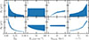 |
Fig. C.1. Range of magnetic field strengths in the sightlines of image A and image B calculated with different parameter ranges for ionization fractions (panels a and b), electron column densities assumed at the position of image A (panels c and d), magnetic scale heights (panels e and f), and inclinations (panels g and h). |
Assumed ranges of the parameters for the lensing galaxy of B1600+434.
C.1. Ionization fraction
We change the ionization fraction (fion) from 0.05 to 0.5 (shown in panels a and b of Fig. C.1) while keeping the other parameters in the MW parameter range. We find that the magnetic field strength decreases exponentially with increasing ionization fraction (as in the case of higher fion, more of the observed RM difference can be explained by high electron densities instead of strong magnetic fields). If we assume fion = 0.05, the derived magnetic field strength can be ∼10 times larger than with fion = 0.5. We can see this effect even in our MW parameter range; the lowest value of fion (0.07) can result in a B field strength around double that of the one calculated with its highest value (fion = 0.014).
C.2. Electron column density at the position of image A
We vary the electron column density at the position of image A (Ne, A) over 1–100 pc cm−3 (shown in panels c and d of Fig. C.1), while keeping the other parameters in the MW parameter range. We set fion to 10%, to exclude changes due to changes in the ionization fraction, since we saw in Appendix C.1 that a change in the assumed ionization fraction can significantly affect our derived magnetic field strength. We find that the lower boundary on the range of magnetic field strengths at the position of image B decreases with higher Ne, A: the B field strength can be three times lower in the case of Ne, A = 100 pc cm−3 compared to Ne, A = 1 pc cm−3. In the case of the B field strength at the position of image A, we do not find a strong dependence on Ne, A; here the wide range is due to the different geometry models that give very different B field strengths.
C.3. Scale height
We change the scale height (Hhalo) from 2 to 20 kpc (shown in panels e and f of Fig. C.1), while we use the MW parameter range for other parameters, and set fion to 10%. At the position of image B (0.7 kpc from the midplane), the scale height does not significantly affect the derived magnetic field strength; it only increases by 1–3% from Hhalo = 2 kpc to 20 kpc. In the case of the location probed by image A (6.2 kpc away from the midplane), the effect is obviously larger: the magnetic field strength increases by a factor of ∼10 from Hhalo = 2 kpc to 20 kpc.
C.4. Inclination
We explore a wider range of inclinations (i) to highlight the magnitude of effect it can have on the magnetic field strength results. While Maller et al. (2000) measured  , we obtained i = 70° ±3° using the Smart Inclination Evaluation with Neural Network (Kourkchi et al. 2020)8 on CASTLES images from the NICMOS instrument of the Hubble Space Telescope (HST), and Maller et al. (1997) could only constrain it to be larger than 65°. Thus, we vary i between 65° and 85° (shown in panels g and h of Fig. C.1), while keeping other parameters in the MW parameter range and setting fion to 10%. We find that the derived magnetic field strengths increase with increasing inclination by a factor of ∼5 from i = 65° to i = 85°.
Appendix D: The effects of the choice of magnetic field geometry model
Considering our restricted parameter range of Milky Way-like parameters, we see that the different models result in different magnetic field strengths (for the summary of values, see Table 3). The constant fields (both symmetric and antisymmetric) result in (absolute) magnetic field strengths of 1.2–1.8 μG at the positions probed by both images. The exponential models result in a field strength of 1.2–1.8 μG at the location of image B (0.7 kpc away from the midplane) and 0.1–0.9 μG at the location of image A (6.2 kpc away from midplane). The models with simple 1/h scaling also lead to 1.2–1.8 μG at the position probed by image B, but to a low 0.1–0.2 μG at the position probed by image A.
We conclude that all the models give consistent results in the case of the location probed by image B. In the case of the location probed by image A, the models give different results, which can be different by a factor of ∼10. This difference is similar in magnitude to the variation that different parameter assumptions can cause. All derived magnetic field strengths are of a reasonable magnitude, thus it is not possible to exclude any of the models based on our data.
All Tables
Stokes QU fitting results of the two polarized components of B1600+434 for the two lensed images.
QU fitting result of the two images of B1600+434 in L band (original and new data).
All Figures
|
Fig. 1. Near Infrared Camera and Multi-Object Spectrometer (NICMOS) H-band image (top) of the lensing system from Kochanek et al. (1999), and the Stokes I (middle) and polarized intensity (PI, bottom) maps from our VLA data. A and B indicate the lensed images of the background quasar, and G shows the lensing galaxy. The lensing galaxy can only be seen in the NICMOS H image, and is too faint to be detected in our VLA images. The Stokes I and PI maps are 16 MHz channel maps at 3.7 GHz. The beam size is shown in the lower left corner. |
| In the text | |
|
Fig. 2. Clean Faraday depth spectra of image A and image B. |
| In the text | |
|
Fig. 3. QU fitting results for images A (top panels) and B (bottom panels). Top row of each panel: Fractional Stokes parameters (q = Q/I, u = U/I), and fractional polarized intensity (PI/I) as a function of λ2. Bottom row of each panel: u as a function of q, and polarization angle as a function of λ2. The fitted models are overlaid as dashed lines. |
| In the text | |
|
Fig. 4. Comparison of our original and our follow-up data in L band. The top row shows Stokes Q/I (blue) and Stokes U/I (red) of our earlier data (empty circles) and our new data (filled circles) as a function of λ2 for image A (left) and image B (right). We also plot the QU fitting model (dashed lines) derived from the full frequency range of the earlier data. The bottom row shows the residual between the two datasets (qold − qnew, uold − unew). |
| In the text | |
|
Fig. C.1. Range of magnetic field strengths in the sightlines of image A and image B calculated with different parameter ranges for ionization fractions (panels a and b), electron column densities assumed at the position of image A (panels c and d), magnetic scale heights (panels e and f), and inclinations (panels g and h). |
| In the text | |
Current usage metrics show cumulative count of Article Views (full-text article views including HTML views, PDF and ePub downloads, according to the available data) and Abstracts Views on Vision4Press platform.
Data correspond to usage on the plateform after 2015. The current usage metrics is available 48-96 hours after online publication and is updated daily on week days.
Initial download of the metrics may take a while.