| Issue |
A&A
Volume 705, January 2026
|
|
|---|---|---|
| Article Number | A251 | |
| Number of page(s) | 14 | |
| Section | Stellar structure and evolution | |
| DOI | https://doi.org/10.1051/0004-6361/202554310 | |
| Published online | 23 January 2026 | |
A comprehensive study of δ Scuti-type pulsators in eclipsing binaries: Oscillating eclipsing Algols
1
Nicolaus Copernicus Astronomical Center, Polish Academy of Sciences ul. Rabiańska 8 87-100 Toruń, Poland
2
Villanova University, Dept. of Astrophysics and Planetary Sciences 800 East Lancaster Avenue Villanova PA 19085, USA
3
Nicolaus Copernicus Astronomical Center, Polish Academy of Sciences ul. Bartycka 18 00-716 Warszawa, Poland
4
Astrophysics Group, Keele University Staffordshire ST5 5BG, U.K.
★ Corresponding author: This email address is being protected from spambots. You need JavaScript enabled to view it.
Received:
28
February
2025
Accepted:
4
November
2025
Abstract
Eclipsing double-lined spectroscopic binaries (SB2s) hosting δ Scuti-type pulsators offer a unique laboratory for simultaneously constraining stellar geometry and interior structure. In this study, we present a comprehensive analysis of five oscillating eclipsing Algol (oEA) binaries. By combining high-precision, short-cadence TESS photometry with multi-epoch high-resolution spectroscopy, we were able to derive precise stellar and orbital parameters. The frequency power spectra were obtained using residuals from binary modelling. We further investigated the evolutionary history of these systems using a grid of MESA binary evolution simulations. Our analysis suggests that the systems must have undergone either case A or case B mass transfer, with the primary components repositioned in the Hertzsprung–Russell (HR) diagram and now pulsating in the δ Scuti regime, while the cooler secondaries are underluminous and inflated, filling their Roche lobes. This study contributes to the growing catalog of well-characterised oEA systems and our understanding of the effects of mass-transfer on the fate of these short-period binaries.
Key words: binaries: eclipsing / stars: oscillations / stars: variables: delta Scuti
© The Authors 2026
 Open Access article, published by EDP Sciences, under the terms of the Creative Commons Attribution License (https://creativecommons.org/licenses/by/4.0), which permits unrestricted use, distribution, and reproduction in any medium, provided the original work is properly cited.
This article is published in open access under the Subscribe to Open model. This email address is being protected from spambots. You need JavaScript enabled to view it. to support open access publication.
1. Introduction
Eclipsing binaries (EBs) that are also double-lined spectroscopic binaries (SB2s) are essential for determining absolute stellar parameters. Their light curves (LCs) constrain geometric configurations relative stellar radii and orbital separation, and provide strong constraints on inclinations (Murphy et al. 2018). Accurate mass determination requires full-phase radial-velocity (RV) coverage, demanding extensive spectroscopic follow-up. This becomes particularly challenging for longer-period systems, where achieving adequate phase coverage requires long baselines and careful scheduling (Torres et al. 2010). Combining precise photometry and spectroscopy yields accurate mass and radius estimates, making EBs key for testing stellar-evolution models. However, these parameters alone leave internal structure, energy transport, and composition largely unconstrained.
Stellar oscillations, driven by intrinsic mechanisms, cause observable brightness variations. In the case of δ Scuti-type stars, classical pulsators with typical masses of 1.5–2.0 Msun, are more frequently found in EBs (Liakos & Niarchos 2017a,b; Kahraman Aliçavuş et al. 2017, 2022a; Chen et al. 2022; Kahraman Aliçavuş et al. 2023). These systems provide precise geometric constraints and enable asteroseismic analysis of the pulsating components (Liakos & Niarchos 2020; Miszuda et al. 2022).
In cases where ground-based data have lacked the precision and continuity to study complex pulsation spectra, space-based photometry from Kepler (Koch et al. 2010) and TESS (Ricker et al. 2015) has enabled detailed analysis of pulsators in EBs.
The remarkable success of Kepler and TESS has led to the discovery of over 1000 δ Scuti-type pulsators in EBs. However, absolute parameters remain difficult to determine, with only ∼10% of systems precisely characterised (Liakos 2024). Several catalogs (Liakos & Niarchos 2017c; Kahraman Aliçavuş et al. 2017; Antoci et al. 2019; Chen et al. 2022; Kahraman Aliçavuş et al. 2022b) and studies (e.g. Murphy et al. 2018) have examined their statistical properties, revealing empirical links between the physical, orbital, and pulsational parameters.
A subset of these binaries consists of short-period, semi-detached systems with extreme mass ratios, indicating prior mass transfer (MT). The MT process alters the lifetimes, temperatures, and luminosities, shifting stars’ positions on the Hertzsprung–Russell (HR) diagram. The classification of MTs is distinguished by Case A, B, or C, depending on whether the donor is on the main sequence, post-main sequence, or asymptotic giant branch, respectively (Kippenhahn & Weigert 1967; Paczyński 1971; Eggleton 2006). In case A, the donor loses mass while core hydrogen burning, potentially evolving into a helium white dwarf or hot subdwarf, depending on core mass, MT efficiency, and mass ratio (Han et al. 2002, 2003). In Case B, MT begins after core hydrogen exhaustion and before helium ignition, producing a helium white dwarf or helium-burning star that later becomes a carbon–oxygen white dwarf. In both cases, the gainer gains mass, accelerating its evolution. Case C occurs when the donor fills its Roche lobe after helium exhaustion, often triggering dynamically unstable MT.
Our sample includes semi-detached Algol-type EBs with pulsating components, which are systems shaped by interaction and distinct from δ Scuti stars in detached EBs (Mkrtichian et al. 2002). Mkrtichian et al. (2004) termed these systems as oscillating eclipsing Algols (oEAs). Studies by Mkrtichian et al. (2018), Lehmann et al. (2020), and Mkrtichian et al. (2022) have advanced our understanding of the physical processes associated with mass transfer (MT) in oEA systems. The 2018 and 2020 works linked magnetic activity cycles to variations in MT and accretion, modulating the pulsation amplitudes across all modes. The authors proposed that the magnetic field in the spot, detected at the Lagrangian point L1 point in the oEA star RZ Cas, along with the Wilson effect in this spot, are mechanisms that regulate the variable feeding of the L1 point and, consequently, mass transfer in Algols. Mkrtichian et al. (2022) and Shi et al. (2022) cataloged known oEA systems and reported new TESS discoveries, underscoring the importance of incorporating time-variable accretion into pulsation and evolutionary models.
One major challenge in characterising these systems is the lack of high-quality RV data, which are essential for deriving precise stellar masses. This limitation persists despite the availability of extensive photometric LCs from surveys, which alone cannot yield absolute parameters. Without RVs, our understanding remains incomplete–like a bottle of finely aged wine, enticingly within reach, yet sealed by the unyielding cork of missing RV measurements.
The Comprehensive Research with Échelles on the Most Interesting Eclipsing Binaries project (CRÉME; Hełminiak et al. 2012, 2015, 2021; Ratajczak et al. 2013) was launched to address this gap. It systematically monitored over 350 EBs, obtaining multi-epoch spectra to refine their fundamental parameters.
In this paper, we present a detailed analysis of five oEA systems from the CRÉME sample. Sections 2 and 3 describe the data collection and curation process, followed by RV and LC modeling. Using the derived system parameters, we performed a frequency analysis on residuals and conduct evolutionary modelling. We conclude with a discussion of our results.
2. Target selection and observations
To identify potential δ Scuti-type pulsators, the systems were pre-selected based on their projected minimum masses, ensuring they fell within the expected mass range for these pulsators. Among these, five systems with exceptionally low mass ratios stood out as strong oEA candidates: TIC 64437380 (HD 139774), TIC 82474821 (SW Pup), TIC 126945917 (HD 202042), TIC 10756751 (GP Cet), and TIC 37817410 (TZ Eri). Among these, TIC 10756751 (GP Cet; Shi et al. 2022), and TIC 37817410 (TZ Eri; Mkrtichian et al. 2006; Liakos & Niarchos 2009) have been previously identified as pulsating oEA stars. Such systems provide valuable opportunities to study the effects of MT on pulsations and binary evolution in semi-detached configurations.
2.1. Photometry
TESS (Ricker et al. 2015) provides 2-min cadence LCs for all the targets in this study. These LCs were retrieved from the Mikulski Archive for Space Telescopes (MAST) using the LIGHTKURVE package (Lightkurve Collaboration 2018). This short cadence photometry ensures that we were able to detect all the high frequency oscillations, which is especially beneficial for pulsators such as δ Scuti-type variables. LCs obtained from multiple TESS sectors provide a longer time baseline which ensures a good accuracy on the detected frequencies. The photometric 2-min cadence data are summarised in Table 1.
Basic information about the targets.
We selected the Simple Aperture Photometry (SAP) flux values for all the targets to avoid distortions in the LCs introduced through Pre-search Data Conditioning (PDC)-SAP fluxes. The data were converted to normalised fluxes and cleaned for long term trends using the WOTAN Python package (Hippke et al. 2019). LCs of all five targets used in this study are shown in the Figure 1.
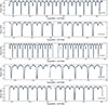 |
Fig. 1. Short (2-min) cadence LCs of the targets, each for a single TESS sector. |
2.2. High resolution spectra
For the calculation of RVs and determination of atmospheric parameters we used high-resolution spectra, obtained with various spectrographs. Their summary is given in Table 1.
Most of the spectra used for analysis were taken with the FEROS spectrograph (Kaufer et al. 1999), attached to the MPG-2.2 m telescope in La Silla. With an image slicer this instrument provides a resolution of ∼48 000. The data were reduced with the CERES pipeline (Brahm et al. 2017), which provides wavelength-calibrated and barycenter-corrected spectra. We used 20 echelle orders, spanning 4135–6500 Å.
Second important source of data was the CHIRON spectrograph (Tokovinin et al. 2013), attached to the 1.5 m SMARTS telescope installed at Cerro Tololo Inter-American Observatory (CTIO). Aiming for a higher level of efficiency, the spectrograph was used in the fiber mode, providing a resolution of ∼28 000. Extracted and wavelength-calibrated spectra were obtained with the pipeline developed at Yale University (Tokovinin et al. 2013) and provided to the user. However, barycentric velocity corrections were done in-house using the bcvcor procedure within IRAF (Tody 1986). About forty echelle orders (4500–6500 Å) were combined and continuum normalised (in IRAF) to be used for RV and spectral analysis.
One system, TIC 10756751 = GP Cet, has been additionally observed with two other facilities: the HIDES spectrograph (R ∼ 55 000; Izumiura 1999), attached to the OAO-188 telescope of the Okayama Astronomical Observatory (Japan), and the IRCS camera/spectropraph (R ∼ 18 000; Kobayashi et al. 2000) behind the Subaru telescope, located at Maunakea (Hawaii). Data reduction and analysis are described in details in Hełminiak et al. (2016) and Hełminiak et al. (2019) for HIDES and IRCS, respectively.
3. Spectroscopy
RV measurements are needed to estimate the dynamical masses of stars. These RVs, derived from the Doppler shifts of spectral lines in observed spectra, directly reflect the stars’ orbital motions. Additionally, estimates of effective temperature and surface gravity obtained from spectral analysis serve as valuable cross-checks for parameters such as flux ratios and relative radii derived from LC modelling.
3.1. Radial velocities
To calculate the RV values, we used the two-dimensional cross-correlation technique implemented in the TODCOR programme (Zucker & Mazeh 1994). Synthetic spectra used as templates were calculated using the ATLAS9 model atmosphere (Kurucz 1979). Errors were calculated using a bootstrap approach (Hełminiak et al. 2012).
Orbital solutions for the extracted RVs were calculated using V2FIT (Konacki et al. 2010). The routine estimates the orbital parameters of a double-Keplerian orbit fitted to the data, using a Levenberg-Marquardt scheme. In the case of TIC 82474821, a clear Rossiter-Mclaughlin effect (Rossiter 1924) was observed. We chose to discard the RVs affected by this to improve the orbital solution.
In general, we fit for the orbital period, Porb, time of periastron passage Tp, systemic velocity, γ, velocity semi-amplitudes, K1, 2, eccentricity, e and longitude at periastron passage, ω. However, in this work we were able to omit the last two parameters, as the orbits were found to be circular (e = 0) in preliminary fits. The orbital fits are displayed in Fig. 2. The less massive star in all the cases is also much fainter and hence displays larger errors in the derived RV values.
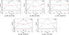 |
Fig. 2. Orbital fits obtained for the RV curves for the targets. Here, primary refers to the more massive star and secondary is the less massive companion. The phase 0 is set to the time of the first quadrature for circular orbits. |
3.2. Broadening functions
In the context of spectral disentangling and fitting, we resorted to broadening functions (BFs), mainly to obtain two necessary parameters: the rotational velocities of the stars and their light contributions. The BF depicts the spectral profiles in velocity space, containing the signatures of RV shifts across various lines, along with intrinsic stellar phenomena such as rotational broadening, spots, and pulsations (Rucinski 1999). The implementation of this method is described in detail in Moharana et al. (2023).
For all five cases, the flux contribution from the fainter secondary is much smaller than from the primary. The noisy nature of the BFs for the secondary components forced us to use this analysis only for the primary stars. The rotational velocities for the primary components are provided in Table 2.
Parameters of the five oEA systems obtained via a combination of LC modelling and spectral analysis.
3.3. Spectral disentangling and analysis
The observed spectrum can be disentangled into the individual spectra of both stars, allowing for an independent analysis of their atmospheric parameters. One approach is to obtain spectra at different orbital phases, where Doppler shifts cause each star’s spectrum to shift within the composite spectrum. By combining multiple spectra with their associated RVs, it is possible to reconstruct the individual component spectra without relying on templates.
Spectral disentangling becomes challenging when phase coverage is sparse or when one component is significantly fainter, leading to a lower signal-to-noise ratio (S/N). Unfortunately, this applies to all targets in our sample. As a result, we could not estimate the light ratio using BFs. Instead, we calculated the passband luminosities for both components in our LC model (see Sect. 4) and used their light ratio for the disentangling process.
We performed spectral disentangling using the DISENTANGLING_SHIFT_AND_ADD code (Shenar et al. 2020, 2022) over the 500–580 nm wavelength range. This selection avoided broad-wing features while ensuring the presence of sufficient narrow lines with adequate S/N. The used RV semi-amplitudes were obtained with V2FIT. For further analysis, we proceeded with only the disentangled primary spectrum, continuum-corrected using the SUPPNET package (Różański et al. 2022)1.
3.4. ISPEC
We used the ISPEC framework (Blanco-Cuaresma et al. 2014; Blanco-Cuaresma 2019) to determine the astrophysical parameters of the disentangled primary spectrum. When necessary, minimal continuum normalisation was performed within ISPEC using third-order splines, and slight RV shifts were also corrected.
From the multiple options provided by ISPEC for spectral fitting we use the ability to generate synthetic spectra on the go using several choices of radiative transfer codes. Specifically, we chose SPECTRUM (Kaufer et al. 1999) for its speed and accuracy along with ATLAS9 plane-parallel model atmospheres (Kurucz 2005). We used the line lists from the Gaia-ESO Survey covering the wavelength range 420–920 nm, and solar abundances from Asplund et al. (2009). ISPEC uses χ2 minimisation to choose the best-fit from the ones generated by SPECTRUM and the observed spectra.
During the fitting process, we fixed the spectral resolution to the instrumental value, and log(g) to the value from LC modelling (Sect. 4) to minimise the degeneracy in fitted values. We perform the fitting procedure using the line lists best suited for determining atmospheric parameters (provided within ISPEC) and we fit for Teff, vsin(i) and microturbulent velocity (vmic). The limb-darkening coefficients are adapted from Claret (2017). We did not perform any further analysis to fit for individual chemical abundances.
3.5. Grid search in stellar paramters (GSSP)
To verify the secondary temperatures obtained using the temperature ratio parameter values from the LC fitting results (Sect. 4), we use the GSSP_COMPOSITE module of the Grid Search in Stellar Paramters (GSSP) software package (Tkachenko 2015). It uses the method of atmosphere models and spectrum synthesis, which performs a comparison of the observations with theoretical spectra from the grid. These synthetic spectra are calculated using the SYNTHV LTE-based radiative transfer code (Tsymbal 1996) and a grid of atmospheric models pre-computed using LLMODELS (Shulyak et al. 2004).
We initiated the primary temperature at the value estimated using ISPEC and fit for the Teffs, vsin(i), and (vmic). The best-fit values of the parameters are mentioned in Table 2. The errors are assumed to be the step size of the parameter grid used to generate the synthetic spectra. The spectral fits are shown in Figure 3.
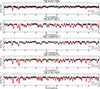 |
Fig. 3. Observed composite spectrum (blue) of the superimposed targets with the GSSP model spectrum (in red) corresponding to the atmospheric parameters from Table 2. |
4. Light curve modelling
Stars in binaries with short orbital period influence each other with significant gravitational forces. These strong tidal forces cause ellipsoidal deformations that are visible in their LCs. These effects can be modelled precisely using the Roche geometry (Eggleton 1983). This treatment also allows to calculate if the stars will fill their respective Roche lobe beyond the point at which mass of the star is no longer gravitationally bound to it. This result, in turn, allows us to reproduce accurate semi-detached and contact binary configurations and their observational signatures in LCs.
The PHOEBE2 (Prša et al. 2016; Horvat et al. 2018; Conroy et al. 2020) incorporates the Roche geometry to model EBs. It also provides treatment for limb darkening laws, third light, and stellar spots, making it physically precise and thus suitable for modelling the high-precision TESS LCs of oEAs.
However, if one or both the stars in the EB harbor rapidly evolving spots, the process of obtaining a binary model becomes more challenging. This prevents us from having a single model for all the sectors as the spot parameters may affect the stellar and orbital parameter values if they are not taken into account. All the systems show signs of activity in the observation window. For each target, we initially selected the sector where minimal spot activity in the form of the O’connell effect (Roberts 1906; O’Connell 1951; Milone 1968) is visible in the LCs. We use these LCs to calculate our primary model.
We set the mass ratio (q) and the projected semi-major axis asin(i) to the values obtained from the RV solutions. The limb darkening coefficients are determined according to the study by Claret (2017), while the gravity darkening coefficients were set to 1 for the primary star with radiative envelope and 0.32 for the secondary star with convective envelope. We found that using 2500 triangles to discretise the surface of each star was a good balance between accuracy and computational efficiency.
When constructing the forward model, we apply the semi-detached constraint provided in the code, ensuring that the equivalent radius reaches its maximum value, corresponding to the star filling its Roche lobe. The forward model was then optimised using a combination of Nelder-Mead and differential evolution optimisers within PHOEBE2. The fitted parameters include the radii ratio, effective temperature ratio, passband luminosity, and orbital inclination.
In some cases, when using semi-detached configuration, we encountered convergence issues at the edge of the Roche tails. To mitigate these errors, we switched to a detached configuration, setting the radius of the secondary star as close as possible to the value of largest possible equivalent radius constrained by the Roche configuration – without triggering errors – before proceeding with the optimisation runs.
The errors were estimated using the Markov chain Monte Carlo (MCMC) sampling, implemented in PHOEBE2 via the EMCEE sampler (Foreman-Mackey et al. 2013). The primary parameters for which we assessed uncertainties included ratio of the stellar radii, inclination, passband luminosity, and the temperature ratio. We show the results in Figure 4 and Table 2.
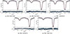 |
Fig. 4. Results of the LC modelling of the systems using the PHOEBE2 software. Upper panel(s): Phased TESS LC (blue) with the best-fitting model superimposed (red). Lower panel(s): Residuals from the fitting procedure. |
5. Eclipse timing
Precisely measured eclipse timings of eclipsing binary star systems can help track any temporal variability that could arise as a result of various dynamical factors. For example, large-scale MT events can alter the orbital momentum, while the gravitational influence of a tertiary companion can perturb the binary’s orbit. Additionally, stellar spots can induce timing variations; in such cases, the O–C diagram of the eclipse minima typically shows an anti-correlation between the primary and secondary eclipses.
Historical mid-eclipse timings for targets TIC 82474821 (SW Pup), TIC 10756751 (GP Cet), and TIC 37817410 (TZ Eri), compiled from several observational programmes, are available at the Up-to-date Linear Elements of Close Binaries database (Kreiner 2004). A detailed investigation on period changes in TZ Eri by Wang et al. (2019) identified both long- and short-term trends, which were interpreted as a combination of mass transfer, angular momentum loss, and the light travel time effect (LTTE; Irwin 1952, 1959).
We extracted mid-eclipse times for all five targets to facilitate potential future studies of timing variations. Primary and secondary minima (see Appendix A) were determined using the method of Marcadon & Prša (2024). Since historical minima timing data are unavailable for our targets, this analysis is based solely on the available TESS observations. The O–C values are computed using the following equation:

where T0 is the adopted initial epoch for each dataset (indicated in the tables as Cycle 0), P is the orbital period, and E is the cycle number.
6. Binary evolution
The process of mass-transfer changes the most important characteristic feature of a star that determines its evolution. The state of the stars in an Algol-type system is not representative of the evolution that a similar mass star would go through. The mass gainer goes through a change in the structure and composition of its outer layers. This process also changes the orbital configuration of the binary system by means of change in angular momentum.
To account for these effects, when we are performing the theoretical modelling process, we need to consider the binary interaction when simulating evolution of this type of star system. To do so, we used the MESA-BINARY module within the Modules for Experiments in Stellar Astrophysics (MESA, Paxton et al. 2011, 2013, 2015, 2018, 2019; Jermyn et al. 2023, version 23.05.1) code to construct models under the non-rotating approximation.
The MESA code builds upon the efforts of many researchers who have advanced our understanding of physics and relies on a variety of input microphysics data. The MESA EOS is a blend of the OPAL (Rogers & Nayfonov 2002), SCVH (Saumon et al. 1995), FreeEOS (Irwin 2004), HELM (Timmes & Swesty 2000), and PC (Potekhin & Chabrier 2010) EOSes. Radiative opacities are primarily from the OPAL project (Iglesias & Rogers 1993, 1996), with data for lower temperatures from Ferguson et al. (2005) and data for high temperatures, dominated by Compton-scattering from Buchler & Yueh (1976). Electron conduction opacities are from Cassisi et al. (2007). The nuclear reaction rates are from JINA REACLIB (Cyburt et al. 2010) plus additional tabulated weak reaction rates from Fuller et al. (1985), Oda et al. (1994) and Langanke & Martínez-Pinedo (2000). Screening was included via the prescription of Chugunov et al. (2007). Thermal neutrino loss rates were taken from Itoh et al. (1996). The MESA-BINARY module allows for the construction of a binary model and the simultaneous evolution of its components, taking into account several important interactions between them. In particular, this module incorporates angular momentum evolution due to MT. Roche lobe radii in binary systems were computed using the fit of Eggleton (1983). The MT rates in Roche lobe overflowing binary systems are determined following the prescriptions of Ritter (1988) and Kolb & Ritter (1990).
To reproduce the evolution of the system, we built an extensive grid of evolutionary models. We constructed a set of varying parameters; namely, initial orbital period, initial masses of the components, metallicity, overshooting from the convective core, mixing-length theory scaling coefficient and a fraction of mass lost during MT, with the ranges as given in Table 3. From this set we constructed vectors of initial parameters with the assumed numerical accuracy (see last column of Table 3) and calculated the evolutionary tracks. The parameters were chosen randomly from uniform distributions within the given ranges. All of these parameters were chosen independently of others, except for the masses. The masses were varied between 0.5 M⊙ and 2.5 M⊙, ensuring that the mass of the primary star was larger than that of the secondary. We tested the mass transfer loss rate from the system by varying the fraction of mass lost from the vicinity of the gainer via isotropic re-emission, exploring values in the range β = 0.0 to β = 0.3. We used Kolb & Ritter (1990) MT prescription and assumed a constant eccentricity e = 0 throughout the system’s evolution. The initial orbital periods in our models were set between 1.2–5 days.
Summary of the parameter ranges and sampling precision used in the evolutionary modeling of the five oEA systems.
In our evolutionary computations, we used the AGSS09 (Asplund et al. 2009) initial chemical composition of the stellar matter and the OPAL opacity tables. These tables were supplemented with data from Ferguson et al. (2005) for lower temperatures. For higher temperatures, hydrogen-poor or metals-rich conditions we used C and O enhanced tables. To determine the chemical composition of stars we varied the value of metallicity Z, from 0.01 to 0.03 and used the linear scaling relations (e.g. Choi et al. 2016), expressed as
with primordial helium abundance of Yp = 0.249 (Planck Collaboration XIII 2016) along with Yprotosolar = 0.2703 and Zprotosolar = 0.0142 proto-solar abundances (Asplund et al. 2009).
Convective instability was treated using the Ledoux criterion, combined with the mixing length theory based on the Henyey et al. (1965) model, employing a mixing-length parameter between αMLT = 0.5 and αMLT = 1.8. In regions that were stable according to the Ledoux criterion but unstable by the Schwarzschild criterion, we applied semi-convective mixing using a scaling factor of αsc = 0.1, following the formalism of Langer et al. (1985). To address regions exhibiting inversion in the mean molecular weight, such as those formed during mass accretion, we applied thermohaline mixing using the formalism of Kippenhahn et al. (1980), with an αth = 1 coefficient. As our models did not include rotational mixing, we introduced a minimum diffusive mixing coefficient of D = 10 cm2 s−1 to smooth out the numerical noise or discontinuities in the internal profiles. Additionally, we accounted for overshooting beyond the formal convective boundaries, using an overshooting parameter, fov, to capture turbulent motions extending into the radiative zone. We applied an exponential overshooting scheme by Herwig (2000) on the top of the H-burning core with changing value from fov = 0.001 to fov = 0.03.
We also accounted for the effects of stellar winds. Our models include wind mass loss, based on the prescriptions of Vink et al. (2001), Reimers (1975) and Blöcker (1995), depending on the effective temperature and the evolutionary stage of a star. For these prescriptions, we adopt efficiency coefficients of ηV = 0.1, ηR = 0.5, and ηB = 0.1, respectively.
Our intention was to apply the aforementioned grid to all systems analysed in this paper. To achieve this, we established a comprehensive grid of 5000 models, calculated based on the parameter ranges outlined in Table 3. This grid served as a foundation for our analysis, allowing us to explore a wide spectrum of stellar configurations. From this initial grid, we carefully selected time steps for each system, that correspond to the values of the measured orbital periods within errors. To select the best fits between the observed and theoretical values we calculated the Mahalanobis distance (Mahalanobis 1936) for each selected time step for the masses and radii. Then, for each system we selected models whose values deviated by up to 50% from the observed equivalents, to extract a sample of models that enabled us to constrain the ranges of the initial parameters. This approach led to the creation of additional grids, incorporating models that can be computed for narrower ranges with more stringent error thresholds, up to 10%. We summarise the effects of evolutionary computations for each system in Table A.1 and Figure 5. The orange and blue lines denote the evolutionary tracks for the gainer and donor, respectively, with dots overplotted on each track, to mark the locations of the best-fitting timestamps. The observed positions are indicated by the error boxes. The lower panels display the evolution of masses, radii and the orbital period with the x-axes representing the evolutionary time (τ) normalised to the current age (τsys) of the corresponding best-fit model. For the readers’ convenience, we show the slow mass transfer phases with thick lines on the HR diagrams. We also provide short descriptions of the results below.
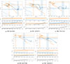 |
Fig. 5. HR diagrams and the evolution of masses, radii, and orbital period for the best-fit evolutionary models of the systems. |
6.1. TIC 82474821.
We identified 16 models that match the observed parameters within 10% of its components’ masses and radii. Some solutions suggest Case A MT, but the majority indicate that the system was formed via non-conservative case B MT, and that it is 0.5–3 Gyr old. Over its evolution, the initially less massive component accretes mass from it’s companion, leading to mass ratio reversal and to the expansion of the convective core. The donor models align at the ridge of the ending phase of MT, after the exhaustion of core hydrogen, and before the onset of hydrogen burning in the envelope. Depending on the MT case, the gainer models point to either early stages of core rejuvenation (case B, where the central hydrogen abundance increases to approx. 0.7) or much later stages of evolution, with H ≈ 0.2–0.3 in the case of type A MT.
6.2. TIC 10756751.
All of the models we were able to establish a fit within 15% of the measured masses and radii of the components. According to these models, TIC 10756751 is likely to have been created from a binary with relatively small orbit, with Porb ≈ 1.2–1.6 d, via an almost conservative case A MT, with up to 10% of transferred mass lost from the system. The system is relatively old, (i.e. 1.86–8.13 Gyr), with the gainer close to terminal age main sequence (TAMS; H ≈ 0.03–0.3) and the donor close to becoming a helium-core pre-white dwarf.
6.3. TIC 37817410.
We found 13 models that fit within 15% of the measured masses and radii of the components, and point to τsys ≈ 1.3–11.2 Gyr. The initial conditions of TIC 37817410 binary are unclear, as wide ranges of initial orbital periods (1.2–2.5 d) and initial masses (1–1.83 M⊙ for the donor, 0.5–0.9 M⊙ for the gainer) are possible. However, some of the best fitting models, point to the over-solar metallicities. In these models, the donor, after transferring a substantial amount of mass to its companion, undergoes an unstable CNO burning cycle in its envelope. This process results in a series of outbursts, occasionally causing the donor to exceed its Roche lobe and triggering brief episodes of additional MT to the companion.
6.4. TIC 64437380 and TIC 126945917.
The best evolutionary models that we were able to identify for TIC 64437380 and TIC 126945917 fit only up to 50% of the components’ masses and radii. We believe that the difficulties in obtaining better fits arise from the parameter ranges chosen for calculating evolutionary tracks, particularly the value of the initial orbital period for the former system and secondary’s initial masses for the latter system (see Table 3). The models we found cluster near the lower limits of the assumed orbital period and masses of the secondary, and the resulting classification of the MT as type B seems to support our hypothesis. We consider that lowering the lower limit of Porb and Macc, ini could lead to the identification of additional models with case A MT, which might improve the overall quality of the fits.
The overall analysis supports the general evolutionary type of each system presented in this paper. After MT starts in, either, case A or B scenario, the initially less massive accretor gains mass, then goes on to build and expand its convective core. On the other hand, the donor after losing a significant fraction of its mass still retains sufficiently thick hydrogen envelope to enter the red giant phase, after which the turbulent CNO burning will cause a series of outbursts, completely washing-out any hydrogen left. Eventually, it will become a He white dwarf.
7. Pulsation analysis
To determine the pulsation frequencies for each system, we used the residuals left over after subtracting the binary model from the LC. To ensure a good frequency resolution we recalculated binary models for the multiple TESS sectors obtaining the longest temporal baseline possible. The binary model is almost never perfect, as the LCs are affected due to spots and pulsations. To ensure that we have minimum contamination from the binary signal during the pulsation analysis, we further cleaned the residuals in two steps. First, we cleaned them for the first 100 harmonics of the orbital frequency. In the next step, we used the WOTAN Python package to remove the long-term trends arising due to imperfect subtraction of spot signals and eclipse ingress+egress profiles. In this step, we cut off the LCs at the eclipses where the detrending was not sufficient.
To perform the time series analysis on these curated residuals, we used v.1.2.9 of the PERIOD04, based on Lenz & Breger (2005). We perform the search for oscillation frequencies from 0 to 80 d−1 to search for δ Scuti-γ Doradus frequencies. A pre-whitening procedure was applied to extract all significant frequencies. The noise level was computed within a 2 d−1 window around each peak, and the signal-to-noise ratio (S/N) was defined as the ratio of the peak amplitude to this average noise amplitude. Only frequencies with an S/N of 5 or greater after pre-whitening were considered significant (Baran et al. 2015; Bowman & Michielsen 2021). We also checked whether the extracted frequency is a combination or a multiplet of other significant frequencies.
All the significant frequencies were then simultaneously fitted using sinusoids to obtain their amplitudes and phases. We show the original periodogram for this curated data and after extraction of all the significant frequencies in Figure 6. A list of all the extracted frequencies, with their analytical errors (Montgomery & O’Donoghue 1999), for each of the systems is provided in Appendix B.
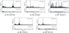 |
Fig. 6. Periodograms for residuals obtained after subtracting binary models from the corresponding LCs. |
To investigate potential tidal perturbations of the extracted frequencies, we constructed Échelle diagrams (Figure 7) using the orbital frequency from Table 2 to compute the Échelle phase. All plots show some frequencies aligned with orbital harmonics, likely due to incomplete removal of the binary signal. Notably, we observe doublets separated by 2forb in the case of TIC 126945917, at the high-frequency end. To check the possibility of these being tidally split modes, we followed the prescription from Jayaraman et al. (2024) to calculate the amplitudes C and phases ϕmult of the combinations,
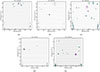 |
Fig. 7. Échelle diagrams with horizontal gray lines marking orbital harmonics. Purple marker indicates dominant frequency and the size of the markers correspond to the amplitude of the frequencies. In the case of TIC 126945917, frequencies forming doublets are specifically marked. |
 (1)
(1)
![Mathematical equation: $$ \begin{aligned} \phi _\mathrm{mult} = a\mathrm{tan}2\left[\frac{A\sin {\phi _{\rm A}-\Phi }+B\cos {\phi _{\rm B}+\Phi }}{A\cos {\phi _{\rm A}-\Phi }+B\cos {\phi _{\rm B}+\Phi }}\right] \end{aligned} $$](/articles/aa/full_html/2026/01/aa54310-25/aa54310-25-eq4.gif) (2)
(2)
where, Φ is the orbital phase, A and B are the amplitudes of the doublet frequencies, while ϕA and ϕB are their phases at an epoch (set to the time of primary minima). The pulsation runs of C and ϕmult are shown in Figure 8. A typical tidally aligned pulsation mode shows amplitude maxima or minima at eclipse phases and simultaneously shows π−jumps, which are quick phase changes of π (Fuller et al. 2020, 2025). They can also show the same variations at maxima of ellipsoidal variations in the out-of-eclipse portions, which is usually due to tidal deformations (Jayaraman et al. 2024). We do not find any amplitude maxima or minima at these specific phases. The same is observed with the phase variations as they have π−jumps but not exactly at any specific orbital phase. This suggests the pulsation axis is misaligned rather than fully aligned with the tidal axis.
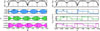 |
Fig. 8. Pulsation runs of the different doublets identified in the Échelle diagram of TIC 126945917. The left panel shows the amplitude variations and the right panel shows the phase variations over the orbital phase. The vertical solid line shows phases of primary eclipse and the dashed vertical lines show the secondary eclipse. |
8. Conclusions
In this study, we present a detailed analysis of five oEA systems selected from the CRÉME survey. By combining high-precision TESS photometry with multi-epoch high-resolution spectroscopy, we derived precise LC and RV solutions that yield precise measurements of the orbital configuration of these binary systems and the fundamental stellar parameters.
The disentangled component spectra were modelled to estimate atmospheric parameters, with solar abundances yielding overall good fits. However, a detailed chemical abundance analysis ought to be performed to further confirm these results.
Our MESA binary evolution simulations suggest that all five systems likely underwent either Case A or Case B mass transfer, and this conclusion is supported by the low mass ratios observed. These findings underscore the significant role that binary interactions and MT play in shaping the evolutionary pathways of intermediate-mass stars.
However, we note that the adopted MESA-BINARY models for our systems do not fully reproduce the observed stellar properties. This discrepancy may arise from various factors, including the treatment of convective overshooting, MT efficiency, angular momentum loss, and stellar rotation. Further refinements are required to better align theoretical predictions with observations, which is crucial for accurately determining the progenitor properties and improving our understanding of the MT process.
We also extracted mid-eclipse times from TESS observations to enable future studies of timing variations. Additionally, analysis of residual LCs revealed multiple significant pulsation frequencies in each system. Preliminary Échelle diagrams suggest possible tidal perturbations in at least one target.
Our results contribute to the growing catalog of well-characterised oscillating EBs, providing essential benchmarks for testing and refining theoretical models of stellar structure and evolution. We aim to extend the asteroseismic analysis of these targets in a future study, specifically mode identification using multi-colour photometry. Seismic modelling will help us further constrain the possible formation scenarios and provide insights on the changes in the internal structure and composition of the stars before and after the MT process and the effect of such MT events on the pulsation properties of the progenitors.
Data availability
Tables A.1–A.5 and B.1–B.5 are available at the CDS via https://cdsarc.cds.unistra.fr/viz-bin/cat/J/A+A/705/A251
Acknowledgments
We thank the anonymous referee for valuable comments that helped improve the manuscript. We acknowledge support provided by the Polish National Science Center through grants no. 2017/27/B/ST9/02727, 2021/41/N/ST9/02746, 2021/43/B/ST9/02972, 2023/49/B/ST9/01671, and 2024/53/N/ST9/03885. A. Moharana acknowledges support from the UK Science and Technology Facilities Council (STFC) under grant number ST/Y002563/1. F. Marcadon acknowledges support from the European Research Council (ERC) under the European Union’s Horizon 2020 research and innovation programme (grant agreement No. 951549) and from the Polish-French Marie Skłodowska-Curie and Pierre Curie Science Prize awarded by the Foundation for Polish Science and the Polish Ministry of Science and Higher Education grant agreement 2024/WK/02. This research made use of data collected at ESO under programmes 088.D-0080, 089.D-0097, 090.D-0061, 091.D-0145, 094.A-9029, as well as through CNTAC proposal 2014B-067. This research is based in part on data collected at Subaru Telescope, which is operated by the National Astronomical Observatory of Japan. We are honored and grateful for the opportunity of observing the Universe from Maunakea, which has the cultural, historical and natural significance in Hawaii. This research made use of Lightkurve, a Python package for Kepler and TESS data analysis (Lightkurve Collaboration 2018). This research uses data collected by the TESS mission (Guest Investigator proposals: G011083, G011154, G03028, G03251, G04047, G04171, G04234, G05003, G05078, G05125, G06057) which are publicly available from the MAST portal. Funding for the TESS mission is provided by NASA’s Science Mission directorate.
References
- Antoci, V., Cunha, M. S., Bowman, D. M., et al. 2019, MNRAS, 490, 4040 [Google Scholar]
- Asplund, M., Grevesse, N., Sauval, A. J., & Scott, P. 2009, ARA&A, 47, 481 [NASA ADS] [CrossRef] [Google Scholar]
- Baran, A. S., Koen, C., & Pokrzywka, B. 2015, MNRAS, 448, L16 [NASA ADS] [CrossRef] [Google Scholar]
- Blanco-Cuaresma, S. 2019, MNRAS, 486, 2075 [Google Scholar]
- Blanco-Cuaresma, S., Soubiran, C., Heiter, U., & Jofré, P. 2014, A&A, 569, A111 [CrossRef] [EDP Sciences] [Google Scholar]
- Blöcker, T. 1995, A&A, 297, 727 [NASA ADS] [Google Scholar]
- Bowman, D. M., & Michielsen, M. 2021, A&A, 656, A158 [NASA ADS] [CrossRef] [EDP Sciences] [Google Scholar]
- Brahm, R., Jordán, A., & Espinoza, N. 2017, PASP, 129, 034002 [Google Scholar]
- Buchler, J. R., & Yueh, W. R. 1976, ApJ, 210, 440 [NASA ADS] [CrossRef] [Google Scholar]
- Cassisi, S., Potekhin, A. Y., Pietrinferni, A., Catelan, M., & Salaris, M. 2007, ApJ, 661, 1094 [NASA ADS] [CrossRef] [Google Scholar]
- Chen, X., Ding, X., Cheng, L., et al. 2022, ApJS, 263, 34 [CrossRef] [Google Scholar]
- Choi, J., Dotter, A., Conroy, C., et al. 2016, ApJ, 823, 102 [Google Scholar]
- Chugunov, A. I., Dewitt, H. E., & Yakovlev, D. G. 2007, Phys. Rev. D, 76, 025028 [NASA ADS] [CrossRef] [Google Scholar]
- Claret, A. 2017, A&A, 600, A30 [NASA ADS] [CrossRef] [EDP Sciences] [Google Scholar]
- Conroy, K. E., Kochoska, A., Hey, D., et al. 2020, ApJS, 250, 34 [Google Scholar]
- Cyburt, R. H., Amthor, A. M., Ferguson, R., et al. 2010, ApJS, 189, 240 [NASA ADS] [CrossRef] [Google Scholar]
- Eggleton, P. P. 1983, ApJ, 268, 368 [Google Scholar]
- Eggleton, P. 2006, Evolutionary Processes in Binary and Multiple Stars [Google Scholar]
- Ferguson, J. W., Alexander, D. R., Allard, F., et al. 2005, ApJ, 623, 585 [Google Scholar]
- Foreman-Mackey, D., Hogg, D. W., Lang, D., & Goodman, J. 2013, PASP, 125, 306 [Google Scholar]
- Fuller, G. M., Fowler, W. A., & Newman, M. J. 1985, ApJ, 293, 1 [NASA ADS] [CrossRef] [Google Scholar]
- Fuller, J., Kurtz, D. W., Handler, G., & Rappaport, S. 2020, MNRAS, 498, 5730 [NASA ADS] [CrossRef] [Google Scholar]
- Fuller, J., Rappaport, S., Jayaraman, R., Kurtz, D., & Handler, G. 2025, ApJ, 979, 80 [Google Scholar]
- Gaia Collaboration (Vallenari, A., et al.) 2023, A&A, 674, A1 [NASA ADS] [CrossRef] [EDP Sciences] [Google Scholar]
- Han, Z., Podsiadlowski, P., Maxted, P. F. L., Marsh, T. R., & Ivanova, N. 2002, MNRAS, 336, 449 [Google Scholar]
- Han, Z., Podsiadlowski, P., Maxted, P. F. L., & Marsh, T. R. 2003, MNRAS, 341, 669 [NASA ADS] [CrossRef] [Google Scholar]
- Hełminiak, K. G., Konacki, M., Różyczka, M., et al. 2012, MNRAS, 425, 1245 [CrossRef] [Google Scholar]
- Hełminiak, K. G., Graczyk, D., Konacki, M., et al. 2015, MNRAS, 448, 1945 [CrossRef] [Google Scholar]
- Hełminiak, K. G., Ukita, N., Kambe, E., et al. 2016, MNRAS, 461, 2896 [CrossRef] [Google Scholar]
- Hełminiak, K. G., Tokovinin, A., Niemczura, E., et al. 2019, A&A, 622, A114 [EDP Sciences] [Google Scholar]
- Hełminiak, K. G., Moharana, A., Pawar, T., et al. 2021, MNRAS, 508, 5687 [CrossRef] [Google Scholar]
- Henyey, L., Vardya, M. S., & Bodenheimer, P. 1965, ApJ, 142, 841 [Google Scholar]
- Herwig, F. 2000, A&A, 360, 952 [NASA ADS] [Google Scholar]
- Hippke, M., David, T. J., Mulders, G. D., & Heller, R. 2019, AJ, 158, 143 [Google Scholar]
- Horvat, M., Conroy, K. E., Pablo, H., et al. 2018, ApJS, 237, 26 [Google Scholar]
- Iglesias, C. A., & Rogers, F. J. 1993, ApJ, 412, 752 [Google Scholar]
- Iglesias, C. A., & Rogers, F. J. 1996, ApJ, 464, 943 [NASA ADS] [CrossRef] [Google Scholar]
- Irwin, J. B. 1952, ApJ, 116, 211 [Google Scholar]
- Irwin, J. B. 1959, AJ, 64, 149 [Google Scholar]
- Irwin, A. W. 2004, The FreeEOS Code for Calculating the Equation of State for Stellar Interiors [Google Scholar]
- Itoh, N., Hayashi, H., Nishikawa, A., & Kohyama, Y. 1996, ApJS, 102, 411 [NASA ADS] [CrossRef] [Google Scholar]
- Izumiura, H. 1999, in Observational Astrophysics in Asia and Its Future, ed. P. S. Chen, 4, 77 [Google Scholar]
- Jayaraman, R., Rappaport, S. A., Powell, B., et al. 2024, ApJ, 975, 121 [Google Scholar]
- Jermyn, A. S., Bauer, E. B., Schwab, J., et al. 2023, ApJS, 265, 15 [NASA ADS] [CrossRef] [Google Scholar]
- Kahraman Aliçavuş, F., Soydugan, E., Smalley, B., & Kubát, J. 2017, MNRAS, 470, 915 [CrossRef] [Google Scholar]
- Kahraman Aliçavuş, F., Gümüş, D., Kırmızıtaş, Ö., et al. 2022a, Res. Astron. Astrophys., 22, 085003 [CrossRef] [Google Scholar]
- Kahraman Aliçavuş, F., Handler, G., Aliçavuş, F., et al. 2022b, MNRAS, 510, 1413 [Google Scholar]
- Kahraman Aliçavuş, F., Çoban, Ç. G., Çelik, E., et al. 2023, MNRAS, 524, 619 [CrossRef] [Google Scholar]
- Kaufer, A., Stahl, O., Tubbesing, S., et al. 1999, The Messenger, 95, 8 [Google Scholar]
- Kippenhahn, R., & Weigert, A. 1967, Z. Astrophys., 65, 251 [NASA ADS] [Google Scholar]
- Kippenhahn, R., Ruschenplatt, G., & Thomas, H. C. 1980, A&A, 91, 175 [Google Scholar]
- Kobayashi, N., Tokunaga, A. T., Terada, H., et al. 2000, in Optical and IR Telescope Instrumentation and Detectors, eds. M. Iye, & A. F. Moorwood, SPIE Conf. Ser., 4008, 1056 [Google Scholar]
- Koch, D. G., Borucki, W. J., Basri, G., et al. 2010, ApJ, 713, L79 [Google Scholar]
- Kolb, U., & Ritter, H. 1990, A&A, 236, 385 [NASA ADS] [Google Scholar]
- Konacki, M., Muterspaugh, M. W., Kulkarni, S. R., & Hełminiak, K. G. 2010, ApJ, 719, 1293 [NASA ADS] [CrossRef] [Google Scholar]
- Kreiner, J. M. 2004, Acta Astron., 54, 207 [NASA ADS] [Google Scholar]
- Kurucz, R. L. 1979, ApJS, 40, 1 [NASA ADS] [CrossRef] [Google Scholar]
- Kurucz, R. L. 2005, Mem. Soc. Astron. Ital. Suppl., 8, 14 [Google Scholar]
- Langanke, K., & Martínez-Pinedo, G. 2000, Nucl. Phys. A, 673, 481 [NASA ADS] [CrossRef] [Google Scholar]
- Langer, N., El Eid, M. F., & Fricke, K. J. 1985, A&A, 145, 179 [NASA ADS] [Google Scholar]
- Lehmann, H., Dervişoğlu, A., Mkrtichian, D. E., et al. 2020, A&A, 644, A121 [NASA ADS] [CrossRef] [EDP Sciences] [Google Scholar]
- Lenz, P., & Breger, M. 2005, CoAst, 146, 53 [NASA ADS] [Google Scholar]
- Liakos, A. 2024, arXiv e-prints [arXiv:2410.00763] [Google Scholar]
- Liakos, A., & Niarchos, P. 2009, CoAst, 160, 2 [Google Scholar]
- Liakos, A., & Niarchos, P. 2017a, MNRAS, 465, 1188 [Google Scholar]
- Liakos, A., & Niarchos, P. 2017b, MNRAS, 465, 1214 [Google Scholar]
- Liakos, A., & Niarchos, P. 2017c, MNRAS, 465, 1181 [NASA ADS] [CrossRef] [Google Scholar]
- Liakos, A., & Niarchos, P. 2020, Galaxies, 8, 75 [NASA ADS] [CrossRef] [Google Scholar]
- Lightkurve Collaboration (Cardoso, J. V. d. M., et al.) 2018, Lightkurve: Kepler and TESS Time Series Analysis in Python (Astrophysics Source Code Library) [Google Scholar]
- Mahalanobis, P. 1936, On the Generalised Distance in Statistics, 2, 49 [Google Scholar]
- Marcadon, F., & Prša, A. 2024, ApJ, 976, 242 [Google Scholar]
- Milone, E. E. 1968, AJ, 73, 708 [Google Scholar]
- Miszuda, A., Kołaczek-Szymański, P. A., Szewczuk, W., & Daszyńska-Daszkiewicz, J. 2022, MNRAS, 514, 622 [NASA ADS] [CrossRef] [Google Scholar]
- Mkrtichian, D. E., Kusakin, A. V., Gamarova, A. Y., & Nazarenko, V. 2002, in IAU Colloquium 185: Radial and Nonradial Pulsations as Probes of Stellar Physics, eds. C. Aerts, T. R. Bedding, & J. Christensen-Dalsgaard, ASP Conf. Ser., 259, 96 [Google Scholar]
- Mkrtichian, D., Kusakin, A., Rodriguez, E., et al. 2004, A&A, 419, 1015 [NASA ADS] [CrossRef] [EDP Sciences] [Google Scholar]
- Mkrtichian, D., Kim, S. L., Kusakin, A. V., et al. 2006, Ap&SS, 304, 169 [Google Scholar]
- Mkrtichian, D. E., Lehmann, H., Rodríguez, E., et al. 2018, MNRAS, 475, 4745 [NASA ADS] [CrossRef] [Google Scholar]
- Mkrtichian, D., Gunsriviwat, K., Lehmann, H., et al. 2022, Galaxies, 10, 97 [NASA ADS] [CrossRef] [Google Scholar]
- Moharana, A., Hełminiak, K. G., Marcadon, F., et al. 2023, MNRAS, 521, 1908 [NASA ADS] [CrossRef] [Google Scholar]
- Montgomery, M. H., & O’Donoghue, D. 1999, DSSN, 13, 28 [Google Scholar]
- Murphy, S. J., Moe, M., Kurtz, D. W., et al. 2018, MNRAS, 474, 4322 [Google Scholar]
- O’Connell, D. J. K. 1951, Publ. Riverview Coll. Obs., 2, 85 [Google Scholar]
- Oda, T., Hino, M., Muto, K., Takahara, M., & Sato, K. 1994, At. Data Nucl. Data Tables, 56, 231 [NASA ADS] [CrossRef] [Google Scholar]
- Paczyński, B. 1971, ARA&A, 9, 183 [Google Scholar]
- Paxton, B., Bildsten, L., Dotter, A., et al. 2011, ApJS, 192, 3 [Google Scholar]
- Paxton, B., Cantiello, M., Arras, P., et al. 2013, ApJS, 208, 4 [Google Scholar]
- Paxton, B., Marchant, P., Schwab, J., et al. 2015, ApJS, 220, 15 [Google Scholar]
- Paxton, B., Schwab, J., Bauer, E. B., et al. 2018, ApJS, 234, 34 [NASA ADS] [CrossRef] [Google Scholar]
- Paxton, B., Smolec, R., Schwab, J., et al. 2019, ApJS, 243, 10 [Google Scholar]
- Planck Collaboration XIII. 2016, A&A, 594, A13 [NASA ADS] [CrossRef] [EDP Sciences] [Google Scholar]
- Potekhin, A. Y., & Chabrier, G. 2010, Contrib. Plasma Phys., 50, 82 [NASA ADS] [CrossRef] [Google Scholar]
- Prša, A., Conroy, K. E., Horvat, M., et al. 2016, ApJS, 227, 29 [Google Scholar]
- Ratajczak, M., Hełminiak, K. G., Konacki, M., & Jordán, A. 2013, MNRAS, 433, 2357 [NASA ADS] [CrossRef] [Google Scholar]
- Reimers, D. 1975, Mem. Soc. R. Sci. Liege, 8, 369 [NASA ADS] [Google Scholar]
- Ricker, G. R., Winn, J. N., Vanderspek, R., et al. 2015, J. Astron. Telesc. Instrum. Syst., 1, 014003 [Google Scholar]
- Ritter, H. 1988, A&A, 202, 93 [NASA ADS] [Google Scholar]
- Roberts, A. W. 1906, MNRAS, 66, 123 [Google Scholar]
- Rogers, F. J., & Nayfonov, A. 2002, ApJ, 576, 1064 [Google Scholar]
- Rossiter, R. A. 1924, ApJ, 60, 15 [Google Scholar]
- Różański, T., Niemczura, E., Lemiesz, J., Posiłek, N., & Różański, P. 2022, A&A, 659, A199 [NASA ADS] [CrossRef] [EDP Sciences] [Google Scholar]
- Rucinski, S. 1999, Turk. J. Phys., 23, 271 [Google Scholar]
- Saumon, D., Chabrier, G., & van Horn, H. M. 1995, ApJS, 99, 713 [NASA ADS] [CrossRef] [Google Scholar]
- Shenar, T., Bodensteiner, J., Abdul-Masih, M., et al. 2020, A&A, 639, L6 [EDP Sciences] [Google Scholar]
- Shenar, T., Sana, H., Mahy, L., et al. 2022, A&A, 665, A148 [NASA ADS] [CrossRef] [EDP Sciences] [Google Scholar]
- Shi, X.-d., Qian, S.-b., & Li, L.-J. 2022, ApJS, 259, 50 [NASA ADS] [CrossRef] [Google Scholar]
- Shulyak, D., Tsymbal, V., Ryabchikova, T., Stütz, C., & Weiss, W. W. 2004, A&A, 428, 993 [NASA ADS] [CrossRef] [EDP Sciences] [Google Scholar]
- Timmes, F. X., & Swesty, F. D. 2000, ApJS, 126, 501 [NASA ADS] [CrossRef] [Google Scholar]
- Tkachenko, A. 2015, A&A, 581, A129 [NASA ADS] [CrossRef] [EDP Sciences] [Google Scholar]
- Tody, D. 1986, in Instrumentation in Astronomy VI, ed. D. L. Crawford, SPIE Conf. Ser., 627, 733 [NASA ADS] [CrossRef] [Google Scholar]
- Tokovinin, A., Fischer, D. A., Bonati, M., et al. 2013, PASP, 125, 1336 [NASA ADS] [CrossRef] [Google Scholar]
- Torres, G., Andersen, J., & Giménez, A. 2010, A&ARv, 18, 67 [Google Scholar]
- Tsymbal, V. 1996, in M.A.S.S., Model Atmospheres and Spectrum Synthesis, eds. S. J. Adelman, F. Kupka, & W. W. Weiss, ASP Conf. Ser., 108, 198 [Google Scholar]
- Vink, J. S., de Koter, A., & Lamers, H. J. G. L. M. 2001, A&A, 369, 574 [NASA ADS] [CrossRef] [EDP Sciences] [Google Scholar]
- Wang, Z.-H., Zhu, L.-Y., Li, L.-J., & Tian, X.-M. 2019, Res. Astron. Astrophys., 19, 107 [Google Scholar]
- Zucker, S., & Mazeh, T. 1994, ApJ, 420, 806 [NASA ADS] [CrossRef] [Google Scholar]
Appendix
Results of the evolutionary computations summarising the initial and final parameters of the models, sorted by fit quality.
All Tables
Parameters of the five oEA systems obtained via a combination of LC modelling and spectral analysis.
Summary of the parameter ranges and sampling precision used in the evolutionary modeling of the five oEA systems.
Results of the evolutionary computations summarising the initial and final parameters of the models, sorted by fit quality.
All Figures
|
Fig. 1. Short (2-min) cadence LCs of the targets, each for a single TESS sector. |
| In the text | |
|
Fig. 2. Orbital fits obtained for the RV curves for the targets. Here, primary refers to the more massive star and secondary is the less massive companion. The phase 0 is set to the time of the first quadrature for circular orbits. |
| In the text | |
|
Fig. 3. Observed composite spectrum (blue) of the superimposed targets with the GSSP model spectrum (in red) corresponding to the atmospheric parameters from Table 2. |
| In the text | |
|
Fig. 4. Results of the LC modelling of the systems using the PHOEBE2 software. Upper panel(s): Phased TESS LC (blue) with the best-fitting model superimposed (red). Lower panel(s): Residuals from the fitting procedure. |
| In the text | |
|
Fig. 5. HR diagrams and the evolution of masses, radii, and orbital period for the best-fit evolutionary models of the systems. |
| In the text | |
|
Fig. 6. Periodograms for residuals obtained after subtracting binary models from the corresponding LCs. |
| In the text | |
|
Fig. 7. Échelle diagrams with horizontal gray lines marking orbital harmonics. Purple marker indicates dominant frequency and the size of the markers correspond to the amplitude of the frequencies. In the case of TIC 126945917, frequencies forming doublets are specifically marked. |
| In the text | |
|
Fig. 8. Pulsation runs of the different doublets identified in the Échelle diagram of TIC 126945917. The left panel shows the amplitude variations and the right panel shows the phase variations over the orbital phase. The vertical solid line shows phases of primary eclipse and the dashed vertical lines show the secondary eclipse. |
| In the text | |
Current usage metrics show cumulative count of Article Views (full-text article views including HTML views, PDF and ePub downloads, according to the available data) and Abstracts Views on Vision4Press platform.
Data correspond to usage on the plateform after 2015. The current usage metrics is available 48-96 hours after online publication and is updated daily on week days.
Initial download of the metrics may take a while.