| Issue |
A&A
Volume 705, January 2026
|
|
|---|---|---|
| Article Number | A190 | |
| Number of page(s) | 21 | |
| Section | Planets, planetary systems, and small bodies | |
| DOI | https://doi.org/10.1051/0004-6361/202556146 | |
| Published online | 22 January 2026 | |
Characterising planetary systems with SPIRou: Questions about the magnetic cycle of 55 Cnc A and two new planets around B★
1
Université de Toulouse, CNRS, IRAP,
14 avenue Belin,
31400
Toulouse,
France
2
Laboratory for Astrophysics, Leiden Observatory,
PO Box 9513,
2300 RA
Leiden,
The Netherlands
3
LIRA, Observatoire de Paris, Université PSL,
5 Place Jules Janssen,
92195
Meudon,
France
4
Canada-France-Hawaii Telescope, CNRS,
Kamuela,
HI
96743,
USA
5
Institut Trottier de Recherche sur les Exoplanètes, Université de Montréal,
1375 Ave Thérèse-Lavoie-Roux,
Montréal,
QC
H2V 0B3,
Canada
6
Université Grenoble Alpes, CNRS, IPAG,
38000
Grenoble,
France
★★ Corresponding author: This email address is being protected from spambots. You need JavaScript enabled to view it.
Received:
27
June
2025
Accepted:
6
October
2025
Abstract
One of the first exoplanet hosts, discovered about thirty years ago, the star 55 Cnc has been continuously observed ever since. It is now known to host at least five planets with orbital periods ranging from 17 hours to 15 years. It is also one of the most extreme metal-rich stars in the neighbourhood, and it has a low-mass secondary star. In this article, we present data obtained at the Canada-France-Hawai’i Telescope with the SPIRou spectropolarimeter on both components of the 55 Cnc stellar system. We revisit the long-period radial-velocity signals of 55 Cnc A, with a focus on the role of the magnetic cycle, and propose the existence of a sixth planet candidate, whose period falls close to that of the magnetic cycle, or half of it. The other massive outer planet has a revised period of 13.15 years and a minimum mass of 3.8 MJup. Although some uncertainty remains about these outer planets, the characterisation of the four inner planets is very robust through the combination of many different datasets, and all signals are consistent in the near-infrared (nIR) and optical domains. In addition, the magnetic topology of the solar-type primary component of the system was observed by SPIRou at the minimum of its activity cycle, characterised by an amplitude ten times smaller than observed that during its maximum in 2017. For the low-mass component 55 Cnc B, we report the discovery of two exoplanets in the system, with a period of 6.799 ± 0.0014 and 33.75 ± 0.04 days and a minimum mass of 3.5 ± 0.8 and 5.3 ± 1.4 M⊕, respectively. The secondary magnetic field is very weak, and the current dataset does not allow its precise characterisation, setting an upper limit of 10 G. The system 55 Cnc stands out as the sixth binary system with planetary systems around both components and the first one with non-equal-mass stellar components.
Key words: planets and satellites: detection / stars: low-mass / stars: magnetic field / planetary systems / stars: individual: 55 Cnc / stars: solar-type
Based on observations obtained at the Canada-France-Hawaii Telescope (CFHT) which is operated by the National Research Council (NRC) of Canada, the Institut National des Sciences de l’Univers of the Centre National de la Recherche Scientifique (CNRS) of France, and the University of Hawaii. The observations at the CFHT were performed with care and respect from the summit of Maunakea which is a significant cultural and historic site.
© The Authors 2026
 Open Access article, published by EDP Sciences, under the terms of the Creative Commons Attribution License (https://creativecommons.org/licenses/by/4.0), which permits unrestricted use, distribution, and reproduction in any medium, provided the original work is properly cited.
This article is published in open access under the Subscribe to Open model. This email address is being protected from spambots. You need JavaScript enabled to view it. to support open access publication.
1 Introduction
The nearby Sun-like star 55 Cnc (also named ρ1 Cnc, HD 75732, HIP 43587, and HR 3522) hosts five known exoplanets. Its planet b, a giant planet in a 14.65 d orbital period, was the fourth exoplanet ever discovered using Lick Observatory radial velocity (RV) measurements (Butler et al. 1997). A few years later, new measurements indicated the presence of other giant planets in the system, notably in the 5110 d and 44 d periods (Marcy et al. 2002). The innermost Neptune-like planet was first found in a 2.8 d period (McArthur et al. 2004; Fischer et al. 2008), which turned out to be the 1 d alias of an even closer and less massive planet at 0.7365 d (Dawson & Fabrycky 2010). This inner planet was subsequently confirmed for its extremely short period and found to be transiting (Winn et al. 2011).
Fischer et al. (2008) further identified a 0.15 MJup planet signal at 260 d. These five planets are thus sorted e, b, c, f, and d in order of their orbital periods. The gap between planets f and d is about 4 au. From Doppler noise estimates in multiple instrument datasets, Baluev (2015) finds indications for an activity cycle of 4599 d in addition to a planet d with a 4825 d period. Two recent RV analyses, including new RV data, revisited the longest-period signals. Bourrier et al. (2018) used the long-period periodicity of stellar chromospheric indices to fix a 3822 d magnetic cycle (using a Keplerian model) and inferred the residual RV signal to planet d at 5574 ± 90 d. Subsequently, Rosenthal et al. (2021) identified two long-period signals at 1966 ± 23 d and 6110 ± 200 d; they assigned the first to a systematic instrumental effect and the second to the magnetic cycle signature, in addition to the 5218 ± 200 d planet d. Finally, Laliotis et al. (2023) provide an update to the data, showing a variation in the S index with a period of 3801 ± 130 d, interpreted as the activity cycle, and report no update on the long-period planet d. Identifying the longest-period signals is thus controversial due to both the complexity of mixing RV data from multiple instruments and the ill-constrained impact of the magnetic cycle. The period of the planet with an approximate 15y orbit is also more difficult to constrain in this context.
Concerning radial velocities, abundant literature data thus exist for this bright northern star, which has been observed by many different instruments. A comprehensive compilation is available in Bourrier et al. (2018) and additional HIRES and APF RV data are published in Rosenthal et al. (2021).
A less massive star is also part of the 55 Cnc stellar system: a mid-M dwarf located at a projected separation of 1065 au, sufficiently distant from the primary that its perturbations should not inhibit planet formation around this companion (see review on planet formation in binaries in Thebault & Haghighipour 2015). The secondary star has been less well studied than its brighter, solar-like counterpart.
In this work, we study the stellar and planetary system as a whole, using recent SPIRou data on both stars and collecting data from the literature. In Section 2, we review the fundamental parameters of both stars. In Section 3, we present SPIRou observations obtained over the past few years. In Sections 4 and 5, we present our analysis of the magnetic properties of the two stars and the two RV time series. Finally, we discuss some of the system’s characteristics in Section 6 and draw our conclusions in Section 7.
2 Stars
2.1 55 Cnc A
The distance to 55 Cnc has been updated by Gaia measurements to 12.590 ± 0.012 pc (Gaia Collaboration 2020). The host star 55 Cnc is known to be super-metal-rich. As a Gaia benchmark star, it has been scrutinised, and its [Fe/H] value has been recently updated to 0.32 ± 0.02 (Soubiran et al. 2024), in agreement with the literature values ranging from 0.25 to 0.45. Apart from its metallicity, its fundamental stellar properties are close to those of the Sun with a stellar density of 1.079 ± 0.005 times the solar density and a mass of 1.015 ± 0.051 M⊙ (Crida et al. 2018), constrained by the precise stellar density derived from transits of planet e, luminosity, and interferometric radius measurements. Stellar evolution models predict two separate solutions at 13.2 Gyr and 31 Myr (Ligi et al. 2016), with a preference for the younger scenario, which corresponds to the interferometrically derived stellar radius. However, the older scenario aligns better with the observed very quiet chromospheric star ( of −5.0 and brightness variations of the order of 1 mmag, as reported in Marcy et al. (2002); Bourrier et al. (2018)). In particular, a rotation period longer than 30 days (see below) is not expected for a 30 Myr solar-type star (e.g. Barnes 2007; Gallet & Bouvier 2013). Stellar models may be less accurate for such high stellar metallicity and fail at predicting the observed mass and radius without ambiguity. We select the configuration for which the age is greater than 10 Gyr.
A mean spectrum of 55 Cnc A (hereafter called template) was obtained from all available spectra observed with SPIRou, after instrumental and telluric corrections had been applied (see section 3.1). For 55 Cnc A, more than 1000 individual spectra were summed up. Using this stellar template spectrum, we subsequently used Zeeturbo to derive the fundamental parameters as well as the small-scale magnetic field of the primary star, as described in Cristofari et al. (2023b). We derive an effective temperature of 5198 ± 31 K, a logg of 4.30 ± 0.05, and a metallicity [M/H] of 0.39 ± 0.10 dex in agreement with Soubiran et al. (2024). The model required line broadening, obtained by a vsini of 1.06 ± 0.23 km/s with a macro-turbulence velocity of 2.86 km/s and a small-scale magnetic field of 250 ± 20 G. More precisely, we find that the filling factor with a null magnetic field represents 87%, while the bin with 2 kG magnetic field represents 13% of the surface. Due to the low magnetic field, no component of higher field strength were included in the fit.
The stellar rotation period, derived from chromospheric or photometric variations, lies in the range of 34 to 43 d (Bourrier et al. 2018; Laliotis et al. 2023). Such a range may be indicative of a certain level of differential rotation, expected in solar-like stars. A rotation period of 39 d was measured by Zeeman Doppler imaging (ZDI) during a spectropolarimetric campaign conducted in 2017 (Folsom et al. 2020) and from Hα equivalent-width time series (Bourrier et al. 2018); this is the value we adopt here. The ZDI analysis also places an upper limit on differential rotation at a level of 0.065 rad.day−1 (Folsom et al. 2020).
It is necessary to better understand the contribution of magnetic activity to the long-term RV modulation. Spectropolarimetry may help. The cycle of a Sun-like star is visible in its circular polarisation map over the years, as observed with spectropolarimeters (e.g. Boro Saikia et al. 2016; Mengel et al. 2016). Obtained from TBL/NARVAL data in 2017 and analysed by Folsom et al. (2020), a previous magnetic map is available for 55 Cnc. The reconstructed large-scale magnetic field of 55 Cnc is mostly poloidal, with 80 (20)% of the magnetic energy in the dipole (the quadrupole, respectively) and an average strength of 3.4 G. Stellar wind modelling estimates the mass-loss rate of 55 Cnc to be similar to the Sun’s, at ∼2 × 10⁻¹⁴ M⊙yr−1.
2.2 55 Cnc B
The stellar companion 55 Cnc B is an M4V star at 1065 au southeast from the most massive component (84” visual separation) (Eggenberger et al. 2004). It has a V magnitude of 13.15 and an H magnitude of 7.93. An effective temperature of 3187 ± 157 K and a mass of 0.265 ± 0.02 M⊙ are reported in the revised TESS input catalogue by Stassun et al. (2019). A high metallicity of [M/H]=0.42 is reported in Houdebine et al. (2016) and an effective temperature of 3226 K in Houdebine et al. (2019). However, a wide range of temperatures and metallicities – spanning from 3000 to 3450 K and from −0.2 to +0.5 dex, respectively1 – is present in the literature for this star. A significant discrepancy in the metallicities for the stars in this system is reported by Marfil et al. (2021), with a negative metallicity reported for 55 Cnc B.
The SPIRou template spectrum was analysed using Zeeturbo, as in Cristofari et al. (2023b), providing us with a global fit of the fundamental parameters and the small-scale magnetic field that could impact the magnetically sensitive lines of the star. This template was obtained from the first 52 SPIRou spectra (see section 3.1). This analysis gives an effective temperature of 3286 ± 31 K, a logg of 4.86 ± 0.05, and an [M/H] of 0.16 ± 0.10 with a vsini of 1.29 ± 0.31 km/s. Here again, a macro-turbulence velocity was fixed to 2.9 km/s for this fit. Figure C.2 shows the posterior distribution of these parameters. The metallicity derived for the two components agrees within 2σ and does not confirm the extreme discrepancy reported by Marfil et al. (2021).
For this star, we only set an upper limit on the unsigned, small-scale magnetic field at < 90 Gauss (3-σ confidence), meaning that less than 1% of its surface has a field larger than 2 kG (parameter a2 in the corner plot). This is the signature of a quiet M star compared to the 44 M star sample of the SPIRou Legacy Survey (Cristofari et al. 2023a), confirming the ‘old system’ option.
Using the absolute magnitude in the K band and the calibrated mass-luminosity relations of Mann et al. (2019), the stellar mass of 55 Cnc B is derived as 0.26 ± 0.02 M⊙. The stellar radius, obtained from the estimated effective temperature, absolute magnitudes, and bolometric corrections (Cifuentes et al. 2020), is found to be 0.27 ± 0.07 R⊙. This results in a 2σ difference in the logg value, with logg derived from these mass and radius values being 4.98 instead of the previously fitted 4.86.
Newton et al. (2016) searched for rotational modulation in Kepler data, with a non-detection and an estimated period longer than 500 d. In Houdebine et al. (2016), a minimum value of Prot/sini of 6.11 ± 3 d was derived from the rotational velocity, which is known to be poorly adapted for slow rotators due to insufficient spectral resolution. Such discrepancy may be explained by the extremely low surface activity level and subsequent non-detection of a rotational modulation.
3 Data
3.1 SPIRou
New data on the 55 Cnc stellar system have been collected with the infrared spectropolarimeter SPIRou, mounted on the Canada-France-Hawaii 3.6 m telescope atop Maunakea, Hawai’i. In one shot SPIRou observes the spectral domain from 0.98 to 2.35 µm at a resolution power of 70k. With its stabilised cryogenic spectrograph and simultaneous wavelength calibration, it is used for precise RV measurements, while the Cassegrain polarimetric unit allows us to simultaneously record the large-scale magnetic field of the star through circularly polarised light (Donati et al. 2020). An observation consists of a series of four consecutive exposures, during which the Fresnel rhombs are rotated in such a way so as to derive the circularly polarised spectrum and the Stokes V profile (Donati et al. 1997a).
The SPIRou spectra and associated calibrations were reduced using the APERO pipeline (Cook et al. 2022), and RVs were extracted using the line-by-line (LBL) method adapted to SPIRou by Artigau et al. (2022). Whenever necessary, the systematics in the data were then suppressed by the Wapiti software, which uses the principal component analysis in the LBL framework (Ould-Elhkim et al. 2023). Moreover, differential effective temperatures from LBL derived products were measured following the method described by Artigau et al. (2024).
The more massive component of the system, 55 Cnc A, was observed as a Sun-like calibration star by the observatory (programme ID Q57 from semesters 22B to 25A). The observations used in the current study were performed in the spectropolarimetric mode with 151 sequences collected from 11 January 2023 to 20 April 2025. Each observation consists of four consecutive exposures of 61.29 s. The S/N per pixel in the H band ranges from 190 to 310 per exposure. Ten exposures have significantly lower S/N values and were discarded from our analysis. Note that additional data of 55 Cnc A, obtained with SPIRou for atmospheric studies of planet e, were not included in this study because they either lack simultaneous wavelength calibration, do not use the circular polarisation observing mode, or both. However, these data do contribute to a better stellar template for 55 Cnc A by co-adding 1032 individual spectra, which in turn improves the telluric correction of each spectrum and ultimately improves RV precision.
The secondary M star was observed through the ‘small sisters’ programme (PI C. Moutou, programme IDs 19AF02, 21AF02, 21BF17, 22AF09, and 25AD08), aimed at finding planets around M stars that are companions to more massive, known planet hosts. Seventy polarimetric sequences were collected from 16 February 2019 to 21 April 2025. Table 1 lists the final stellar parameters adopted for this study.
Adopted parameters of target stars.
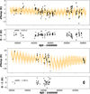 |
Fig. 1 Quasi-periodic GPR model of the differential temperature time series of 55 Cnc A (top) and B (bottom). |
3.2 Archival data
In addition to the SPIRou data, various archival, optical spectra were collected for the chromospheric activity indicator (see Sect. 4.1), longitudinal magnetic field measurements (see Sect. 4.2), and RV analysis (see Sects. 5.1 and 5.2), highlighting the value of long-term open-access datasets. The origin of these data is detailed in the relevant sections.
3.3 Differential temperature
When projected onto a library of stellar templates, SPIRou LBL information can be used to retrieve a disc-averaged differential temperature (dTemp) indicator, which is a proxy for the star’s surface activity. The method is explained in Artigau et al. (2024), where it is valid for effective temperatures ranging from 3000 to 6000 K. Both components of 55 Cnc lie at the edges of the validity domain; nevertheless, examining these data can be instructive.
We modelled the tiny variations in the 55 Cnc A dTemp time series using a quasi-periodic Gaussian process regression (QP-GPR) with the 5500 and 6000 K templates (see Figure 1). We used a kernel whose covariance function is described as
 (1)
with Prot being the rotation period, λe the evolution timescale, and λp the smoothing factor. Subsequently, λe was set to 300 days. Priors for the amplitude and jitter values were set as modified log-uniform functions, ℳℒ𝒰, with initial limits defined from data dispersion. The λp prior is a logarithmic uniform function, ℒ𝒰. These choices are based on Camacho et al. (2023). Table 2 lists the prior and posterior parameters used in the QP-GPR fit. Figure C.3 shows the corner plot. The rotation period of 55 Cnc A is found to be 38.7±0.8 days.
(1)
with Prot being the rotation period, λe the evolution timescale, and λp the smoothing factor. Subsequently, λe was set to 300 days. Priors for the amplitude and jitter values were set as modified log-uniform functions, ℳℒ𝒰, with initial limits defined from data dispersion. The λp prior is a logarithmic uniform function, ℒ𝒰. These choices are based on Camacho et al. (2023). Table 2 lists the prior and posterior parameters used in the QP-GPR fit. Figure C.3 shows the corner plot. The rotation period of 55 Cnc A is found to be 38.7±0.8 days.
Star 55 Cnc B shows a slightly more contrasted dTemp modulation when using the 3000 K or the 3500 K templates. Figure 1 shows the QP-GPR fit to the 55 Cnc B dTemp time series using the 3500 K template, which, at its best fit, exhibits an amplitude of 5 ± 2 K and a period of 92 ± 5 days (see the corner plot in Fig C.4). We used a uniform prior from 3 to 140 days, since no previous estimate of the period was available in the literature.
GPR prior and posterior parameters for differential temperature variations.
4 Magnetic field analyses
4.1 The magnetic cycle of 55 Cnc A
Figure 2 shows when the spectropolarimetric data were collected relative to the chromospheric cycle observed in the CaH and K lines with optical instruments (mainly HIRES, with contributions from HARPS and HARPS-N) (Bourrier et al. 2018; Isaacson et al. 2024). The chromospheric cycle was fitted using a sinusoidal model with a period of 4003 d, which is 2.4σ longer than the 3822±77 d period used in Bourrier et al. (2018) when only one period of the cycle was available.
4.2 Magnetic topology of 55 Cnc A seen by SPIRou
SPIRou was configured in the polarimetric mode during observations of 55 Cnc A. A circularly polarised (Stokes V) spectrum was recorded and reduced for each visit using the APERO reduction pipeline, leading to a total of 131 polarimetric observations. In addition to the near-infrared material, another 62 ptical observations were obtained from the PolarBase archive (Petit et al. 2014), with observations spanning from 2012 to 2018. These observations were obtained with ESPaDOnS at CFHT or its twin NARVAL at the Telescope Bernard Lyot (France).
To increase the S/N, all spectra were processed with the least-squares-deconvolution (LSD, Donati et al. 1997b; Kochukhov et al. 2010) method, using an open source implementation of the algorithm2. The line list used for cross-correlation was extracted from the VALD database (Ryabchikova et al. 2015), using atmospheric parameters close to those of 55 Cnc A. We applied the χ2 criterion of Donati et al. (1997b) to look for the detection of polarised signatures in the line profile, which led to multiple detections of Zeeman signatures in the optical dataset. None of the 131 SPIRou visits led to a definite detection. However, we note that the latest SPIRou run (October 2024 to February 2025) produced statistics closer to the detection threshold.
We computed longitudinal magnetic field (Bl) measurements (Rees & Semel 1979), using the specPolFlow dedicated package3 (Figure 2, bottom panel). A fair fraction of the optical data display Bl absolute values below 1 G, with much larger dispersion observed between December 2016 and December 2017, leading to several Bl absolute values above 2 G and up to 6 G. This period of increased magnetism includes the data presented in the study by Folsom et al. (2020). It is also very close in time to the  maximum reported by Isaacson et al. (2024), confirming that
Folsom’s data were taken at activity maximum (Figure 2, top). In contrast, measurements from 2012, all below 1 G in absolute value, were representative of the  minimum. The SPIRou measurements started close to the subsequent
  minimum, whereas the final SPIRou campaign (October 2024 to February 2025) took place during the expected rise in activity towards a forthcoming maximum. In agreement with this broad picture, early SPIRou measurements are consistent with archival measurements from the previous 2012 minimum. Bl measurements from the latest SPIRou run show increased variability, while the error bars remain at their standard level (of around 0.6 G).
We applied the generalised Lomb-Scargle algorithm (GLS, Zechmeister & Kürster (2009)) to run a period search on the Bl estimates. From the optical data, we obtain a period of 38.6 d, in good agreement with the 39 d period used by Folsom et al. (2020). Using SPIRou observations, the rotation period does not appear, whether using the full time series or subsets. Instead, a peak at around 22 days is recovered, possibly due to the quadrupolar component of the surface field.
We used the ZDI method (Semel 1989; Donati et al. 2006) on SPIRou data to reconstruct the large-scale magnetic geometry of 55 Cnc A. We employed the Python implementation from Folsom et al. (2018a,b). We first checked if, by making use of the full amount of information available in the Stokes V line profiles, the ZDI modelling could detect the rotational modulation of the magnetic signal, since relying on the first moment of Stokes V profiles (Bl estimates, see above) proved inefficient. To do so, we split the full SPIRou dataset into three subsets: 15 observations from January 2023 to May 2023 as subset #1, 76 observations from September 2023 to May 2024 as subset #2, and 40 observations from October 2024 to February 2025 as subset #3. Separating the data into subsets allowed us to characterise the evolution of the magnetic maps over the years while minimising the χ2. We confirmed that modelling the entire time series with a single ZDI map led to an increase in the χ2. The second season with more observations corresponds to the cycle minimum; a test was carried out to see whether the observations in subset #2 could be split into two even parts. The test showed that the two resulting maps were similar and noisier. It was thus optimal to model one map per observing season.
We used an approach similar to that used by Petit et al. (2008, 2022), who computed ZDI models for a range of rotation periods, searching for the period value that would minimise the χ2. The best model was found for a period of 37.9 ± 1.1, 39.8 ± 0.7, and 36.3 ± 0.5 d for subsets #1, 2, and 3, respectively. Since these values are reasonably close to the expected rotation period, we conclude that a rotationally modulated polarised signal can be recovered from the SPIRou observations, even though it is dominated by noise when considering visits individually.
Following this test, we proceeded with ZDI inversion, analysing each subset separately to account for the natural variability in the magnetic geometry. We set our input parameters to the values adopted by Folsom et al. (2020), using Prot = 39 d and v sin i = 1.2 km s−1. Despite an inclination angle likely close to 90◦, we adopted a slightly lower value of 70◦ to limit the mirroring effect reported by Folsom. By doing so, we followed the strategy proposed by Donati et al. (2023) for AU Mic. The resulting maps are shown in Figure 3. For the subsets #1 and #2, we obtain an average unsigned field of 0.3 G, which is nearly ten times weaker than the value obtained by Folsom near activity maximum. For subset #3, the average field increases to about 0.9 G, confirming that 55 Cnc A left its activity minimum before the last SPIRou run. For all subsets, the field geometry is dominated by the poloidal component (storing between 70% and 98% of the magnetic energy). For subsets #1 and #3, the main field component was a dipole, while the quadrupole dominated the geometry in subset #2. At all epochs, the field geometry was mostly non-axisymmetric, with 9% to 37% of the magnetic energy contained in spherical harmonics modes with ℓ = 0. We note, however, that the large inclination angle tends to hide any dipole aligned on the spin axis, since its polar field would be mostly perpendicular to the line of sight (while Stokes V is sensitive to the line-of-sight projection of the magnetic field). The situation would be further complicated by cancelling the polarities in the two hemispheres.
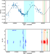 |
Fig. 2 Top: Time variations of the |

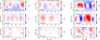 |
Fig. 3 Magnetic geometry of 55 Cnc A. From left to right: ZDI models derived from observations from January to May 2023 (subset #1), September 2023 to May 2024 (subset #2), and October 2024 to February 2025 (subset #3). The stellar surface is shown in equatorial projection, with phases of observation indicated as vertical ticks above the top panel. The vector magnetic field is projected onto a spherical frame, with the radial, azimuthal, and meridional components displayed from top to bottom. The field strength is expressed in Gauss. |
4.3 Magnetic topology of 55 Cnc B
Extracted and reduced with APERO, there are 70 circularly polarised spectra of 55 Cnc B. One sequence, which consisted of repeated trials on the same night at epoch 2460754, was removed due to poor quality, while two other sequences from that night exhibited an average quality. As for the primary star, LSD profiles were calculated from these spectra using a mask built from MARCS models (Gustafsson et al. 2008) of a 3500 K star, keeping atomic lines deeper than 5% of the continuum level, with 408 lines used. None of the Stokes V profiles shows a detected signature, with an average standard deviation of the LSD profile of 4 × 10⁻⁴ in. The integrated, unsigned longitudinal magnetic field in the LSD profiles is less than 10 G at 3σ confidence. There is no significant periodic variability in a GLS periodogram. Figure 4 shows the averaged Stokes profiles of all available 55 Cnc B polarised spectra (consistent with a longitudinal field of 0.6 ± 0.3 G). In conclusion, 55 Cnc B has a low, undetected large-scale magnetic field, in agreement with its low small-scale field, and its topology cannot be characterised from this set of polarised spectra.
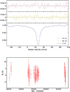 |
Fig. 4 Investigating magnetic field signatures for 55 Cnc B. Top: Intensity (Stokes I), null (Stokes N), and circularly polarised (Stokes V) profiles. Bottom: Variations of the longitudinal magnetic field as a function of time. |
5 Radial velocity analysis
5.1 RV data of 55 Cnc A
The SPIRou RV time series spans 920 days and contains 141 data points. Note that the barycentric Earth RV excursion of ± 29.6 km/s for this star favours a good telluric correction performance (Ould-Elhkim et al. 2026). Also note that the relative motion due to the binary is neglected in this analysis, due to the very large separation (orbital period of about 30 000 years and semi-amplitude of about 200 m/s).
The mean S/N of used RV sequences is 510 per pixel in the H band and the used exposure time is 4 × 61.29s per polarimetric sequence. Table 3 summarises the average SPIRou RV data parameters. The mean error of the SPIRou RV measurements of 55 Cnc A is 0.92 m/s. The K band contributes the least to RV precision, as shown in Table 3.
We then collected literature values. We used the data listed in Bourrier et al. (2018) obtained with various optical spectrographs: Hamilton (290), Tull (141), Keck/HIRES (24+678), and Lick APF (318). We did not use public data from HRS, SOPHIE, HARPS, and HARPS-North, as these were scarce compared to other datasets (mostly acquired for transit observations of planet e). We discarded 19 data points with errors greater than 5 m/s, then binned the data into 2-h bins (sequences for transits or other phases). The total number of visits included in the analysis is 956.
Summary of SPIRou observations.
5.2 RV data of 55 Cnc B
The SPIRou data collection spans 2250 days and contains 69 measurements, mostly obtained after February 2021. Exposure times of 4 × (150 to 400)s per polarimetric sequence were used, depending on the conditions. The mean S/N per pixel in the H band is 180 for the sequences (Table 3). Wapiti corrections were applied to the time series, and we found three principal components that required correction.
Archival RV data exist for this star: 31 measurements from Keck/HIRES (1999–2012) and 11 from CAHA/CARMENES (2016–2020), with an RMS and mean photon noise of 13.62 and 5.3 m/s for HIRES, respectively, and 11.23 and 1.06 m/s for CARMENES (Butler et al. 2017; Ribas et al. 2023). Part of the SPIRou data covers the epoch of the CARMENES observations. The relative motion of the low-mass component is expected with a semi-amplitude of 800 m/s over 30 000 years, which is negligible over the time span of the available measurements.
5.3 Planets around 55 Cnc A
5.3.1 Global analysis
The dispersion is approximately 50 m/s due to known exoplanet signals of large amplitude. The RV time series of 55 Cnc A is modulated by signals of both very short and very long periods, which prevented us from using one instrument only. However, SPIRou data alone with a time span of 920 days is sufficient to independently detect planets e, b, c, and f between 0.73 and 260 d periods, with a residual dispersion of 2.6 m/s or 1.7 m/s when an additional linear trend is fit to account for the second largest signal at 5000 d period.
The first analysis was performed using the tools in DACE (Delisle et al. 2018), which allowed us to easily compare various models. The first model consists of using the planet parameters from Bourrier et al. (2018) to test how it performs with seven more years of RV data. The RMS of the residuals is 6.0 m/s. When the magnetic cycle, fitted as a Keplerian with a 3822 d period, was added, the RMS decreased to 4.5 m/s. The RMS improved to 4.0 m/s when a linear trend was added. This preliminary analysis indicates that the literature model remains robust with the inclusion of an additional seven years of data collection, that a new long-term trend appears, and that the slope in the new SPIRou data is critical to constrain the longest period signals.
A complete analysis was then performed with RadVel version 1.4.11 (Fulton et al. 2018) using the priors from Bourrier et al. (2018). Many models were compared, including those with and without long-term trends, and with varying the priors and number of fitted signals. As in Bourrier et al. (2018), the magnetic cycle was included in the model as an additional Keplerian. The best model was selected from over a dozen other experiments, which included five to seven Keplerian models, linear and quadratic trends, and periodic or quasi-periodic modelling of the stellar cycle.
Concerning the inclusion of stellar activity in the modelling, we faced two main issues. The first is that the main activity indicator, the index derived from the Ca H and K lines, was only available in the past optical data and not in conjunction with the more recent SPIRou data. This lack of continuity required us to extrapolate from the past cycles, as shown in Figure 2, either with a sinusoid or with a Gaussian process. This led to a very imprecise result. The second difficulty arises from the proximity between the (quasi) period of the cycle and the period of one of the Keplerian signals, which forced us to restrain the priors. Consequently, this resulted in ill-constrained models. It is thus a limitation of the present analysis, as long-term entangled signals require longer, homogeneous, combined time series. The favoured model consists of six Keplerians (five for the known planets and one for the possible magnetic cycle) as well as a linear trend.
Each experiment carried out with RadVel also includes a Markov chain Monte Carlo (MCMC) statistical analysis and a Bayesian model comparison in which the significance of all signals is evaluated. The final statistical parameters of the best model are the following: the MCMC chains contained 86 walkers, 7 × 10⁶ steps, and 1.6 × 10⁶ burning steps. The final likelihood value is ln ℒ = −2771. The removal of one of the six modelled signals results in an increase of more than 200 in ln ℒ. The best model is shown in Figure C.6, and the best fit model parameters are listed in Table C.1.
5.3.2 Inner system
The parameters of the four inner planets are remarkably stable compared to the literature values, as expected from the fact that the literature data are heavily used in this analysis and that short-period signals are less affected by the diversity of used instruments. The precision of several parameters is improved with the addition of SPIRou data, with errors on the periods typically twice that of the SPIRou data. Figure 5 shows the individual RV orbits of the planets with the optical (blue symbols) and the nIR/SPIRou (red symbols) RV data, illustrating the lack of chromaticity and similarity. The absence of notable surface RV jitter in this time series allows such a comparison without resorting to Gaussian processes.
We conducted planet injection and recovery tests for a potential planet between planet f and planet d in the O − C residuals. Using a period of 400 days, a planet of 8 M⊕ or more could have been detected.
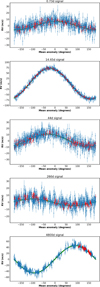 |
Fig. 5 RadVel analysis of 55 Cnc A. Shown are the individual signals, including the five planets. |
5.3.3 Outer system
In the following, we revisit the assumption from Bourrier et al. (2018) that one of the long-term signals is due to the magnetic cycle of the star. In this previous work, the semi-amplitude of the cycle (fitted as a Keplerian with a period of 3822±77 days) is 15.2 ± 1.7 m/s. Here, we find that the best-fit global model favours a  day period signal with a semi-amplitude of 13.06 ± 0.48 m/s, in agreement with the previous analysis and stable over the 28.7 years of data. However, as shown in the previous section, 55 Cnc A is a very quiet star: 1) The rotational modulation is barely seen, or not seen at all, in sensitive activity proxies despite very high S/N values (dTemp, Bl). 2) The large-scale magnetic field strength is 0.3 G during the cycle minimum and up to 3 G during the maximum (possibly hampered due to cancellation between the north and south hemispheres). 3) The mean log
  over 21 years is −5.01 (from data in Isaacson et al. (2024)). This level of activity is lower than the average Sun’s magnetic field, which ranges from 7 to 15 G and exhibits a log
  variation from −5.05 to −4.85 over the 11 year cycle, spanning from minimum to maximum. This variation results in a 2 to 6 m/s scatter (Haywood et al. 2022; Meunier et al. 2010, 2024), mostly due to changes in line shape rather than RV position variability (Klein et al. 2024). In addition, Meunier et al. (2010) mentions an amplitude of 8 m/s, and Meunier & Lagrange (2019) predicts a 1–3 m/s scatter during the stellar cycle of a solar-type star. Other examples in which a magnetic cycle has been identified for stars similar to 55 Cnc A (e.g. the analogues HD 1461, HD 40307, HD 204313, and HD 137388) show a cycle-induced, full RV amplitude of 0.5 to 10 m/s at maximum (e.g. Dumusque et al. 2011; Lovis et al. 2011; Díaz et al. 2016). Finally, we compared optical and nIR RV data over the ∼4000 d variation cycle of 55 Cnc A RVs. They are shown in Figure 6. The signal appears achromatic, with a steep RV increase of about 30 m/s, particularly during the SPIRou observations, which matches the slope observed in previous years with optical spectrographs. Given that SPIRou RVs are measured in a much redder spectral range and during the S index magnetic minimum, such consistent variations and large amplitudes are more indicative of a planetary signal rather than a magnetic cycle. The cycle, however, exists and is probably responsible for part of the RV variation at this 4000 d timescale. If ignored, the derived minimum mass might be slightly overestimated. In Figure 6, the expected cycle signal obtained from the S -index sinusoidal variation is overplotted in light blue. The factor used here between log R′HK and RV is 25 m/s/dex (Meunier & Lagrange 2019). Nevertheless, the factor should rather be 120 m/s/dex to match the observed amplitude at this period. In addition, the period is quite different, and both cycles appear to diverge in recent years. At this point, the absence of chromaticity, the mismatch in periods, and the larger-than-expected amplitude challenge the interpretation of the 3830-d signal as being solely due to the magnetic cycle, suggesting instead that it is mostly caused by another outer planet in the system. Were the entire signal amplitude at this period due to a planet, this would correspond to a minimum mass of 0.9 MJup. It must be noted that other families of solutions rather include a 1900-d signal and a quadratic trend, in addition to the ∼4000 d signal. More data will be needed to confirm the best solution.
The outer planet d is found to have a significantly shorter orbital period of  days compared to
  days (Bourrier et al. 2018), which is 9σ longer. In past studies, the period of this planet was found to be 4905 ± 30 d (Endl et al. 2012), 4825 ± 39 d (Baluev 2015), 5285 ± 5 d (Fischer 2018), and 5218 d (Rosenthal et al. 2021). This apparent instability is obviously linked to the other long-term signal—be it due to the magnetic cycle, a planet, or both—in addition to the fact that the longer signals are naturally more sensitive to the use of multiple instruments than short-period ones. Finally, the best model includes a long-term trend, with a slope of 0.84 ± 0.06 m/s/yr, possibly indicative of another outer body in the system with a period greater than 9000d (24 years). More recent optical RV and S -index data will be published in the future, since this system attracts a great deal of attention. A combined nIR-optical modelling of outer planets and a low-RV-amplitude magnetic cycle will be made possible with the aid of a continuous activity indicator.
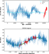 |
Fig. 6 Top: residual RV signal of the sixth Keplerian as a function of time, with all other signals removed. The expected model for the magnetic cycle is superimposed in cyan (see text). Bottom: sixth Keplerian as a function of mean anomaly with the model in green. In both figures, the blue data correspond to all optical RV measurements, and the red data indicates SPIRou nIR RV measurements. |
5.4 Planets around 55 Cnc B
We analysed the 69 RV measurements obtained with SPIRou for 55 Cnc B. SPIRou RV measurements of 55 Cnc B have a mean error of 1.8 m/s and a dispersion of 5.9 m/s. The ℓ1 periodogram (Hara et al. 2017) shows a prominent peak at 6.8d with a logBF4 of 10.3 and a logFAP5 of −0.0015 (Figure 7). Another peak is also present at 33.7 d, with a lower probability. Both periods are different from the rotational period of 92 ± 5 d (Table 2) or the first harmonics of it. The 6.8d and potentially 33.7d signals could thus be due to planetary companions. We subsequently used RadVel to derive the orbital parameters and run an MCMC analysis with one-planet and two-planet models. The best-fit model is shown in Figure 8 together with residuals. The signal is best modelled with the two-planet model in circular orbits with periods of 6.799 ± 0.002 days and 33.747 ± 0.035 d, and semi-amplitudes of 2.89 ± 0.63 m/s and 2.59 ± 0.66 m/s, respectively. RadVel finds a ∆AICc6 improvement of 604 when comparing the the two-planet model to a model with no planets, and it shows a preference for the two-planet model over any one-planet model. The planets causing these RV modulations have a minimum mass of 3.5 ± 0.8 and 5.3 ± 1.4 M⊕, and a semi-major axis of 0.045 ± 0.001 and 0.130 ± 0.003 au, respectively. When the two-planet model is removed, we find no other detected signal in the residuals, including at the rotation period, and the RMS of the residuals is 3.35 m/s. Interestingly, the period ratio is close to 5, which explains the beating pattern in Figure 8. However, this is too great a ratio for active resonance. All parameters for the 55 Cnc B planets are summarised in Table 4.
The available archival data are either too noisy or too scarce to detect the signal seen in the SPIRou data. For example, when the 6.8 d signal was injected 1000 times into the precise but scarce CARMENES data, it was retrieved only 21 times with a FAP smaller than 0.1% (0 times in the HIRES data, and 145 times with both). The complete model is shown in Figure C.7.
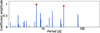 |
Fig. 7 ℓ1 periodogram of 55 Cnc B SPIRou RV data, showing prominent peaks at 6.8 and 33.7 d. |
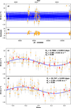 |
Fig. 8 Orbital solution obtained from SPIRou (‘s’) RV data of 55 Cnc B as a function of time (top) and phase (middle and bottom for planets b and c, respectively). The residuals are shown in panel b. Red points are mean measurements per regular 0.1 phase bins as calculated with RadVel when sufficient data is available. |
Fitted parameters for planets b and c of 55 Cnc B.
6 Discussion
6.1 Habitable zones
From this new RV analysis, no new RV signal is detected between the inner set of four planets and the outer planet(s) of 55 Cnc A with a 10 year period or more. The outer part of the habitable zone remains unpopulated at this time. A planet with more than ∼8 M⊕ in a circular 400 d period orbit (or semi-major axis of about 1 au) could be detected in our dataset. However, there remains a suspicion of tentative detections near 1 yr orbital periods. The eccentricity of planet f is 0.063 ± 0.048 in our analysis, slightly smaller than that reported in Bourrier et al. (2018). This confirms and reinforces the dynamical stability of a potential temperate Earth-like planet between 1 and 2 au in the system (Satyal & Cuntz 2019). Although challenging, the detection of a 1–3 M⊕ exoplanet at 1–1.5 au in this complex dataset may be feasible due to the quiet surface of the star but will require several more years of regular observations, both in optical and nIR wavelengths. We note that planet f is also located in the habitable zone of its star in between the runaway and maximum greenhouse limits (Hill et al. 2022), with a minimum mass of about 48.5 M⊕.
Concerning the two planets in the 55 Cnc B system, we find that the first planet has an insolation of 2.6 S⊕ and an equilibrium temperature of 330–370 K, while the second planet has an insolation of 0.3 S⊕ and an equilibrium temperature of 190–210 K, assuming an albedo in the range of 0.50–0.25, respectively. It is safe to say that 55 Cnc Bc lies near the outer edge of the habitable zone of its star, receiving about as much energy as Mars from the Sun. Thus, it seems that the lower mass secondary star of the 55 Cnc system also has at least a temperate planet in its habitable zone extending from approximately 0.055 to 0.14 au. The 55 Cnc system may be the first binary with one planet in each habitable zone.
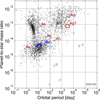 |
Fig. 9 Planet-to-star mass ratio as a function of the orbital period for all known exoplanets. The planets orbiting both components of 55 Cnc are highlighted. The Symbol ‘Ag?’ corresponds to the maximum mass of a planet at a 3830 d period, if confirmed in the future. |
6.2 Planets in binary systems
55 Cnc is only the sixth binary system (out of 739 planet-hosting binaries known to date) in which both stellar components are known to host a planetary system, together with WASP-94 (A and B), Kepler-132 (A and B), XO-2 (N and S), HD 20782 and HD 20781, and HD 113131 (A and B) 7. We stress that this low number is likely strongly biased by the fact that, for a large fraction of planet-hosting binaries, no dedicated investigation of planets around the companion star has been performed. However, it is worth pointing out that among these six systems, 55 Cnc stands out due to the very low mass ratio (0.27) between the two stellar components, while the other five systems have mass ratios close to 1. In fact, 55 Cnc B is one of the smallest known planet-hosting stars that reside in a binary.
Figure 9 presents the planet-to-star mass ratio versus orbital period for the confirmed planets and a potential candidate (marked by ‘Ag?’ and a large ellipse) in the 55 Cnc system, compared to other systems. While the two planets of the secondary join a populated region of this diagram with numerous inner super-Earths, the planets of the primary lie in less populated locations. Comparing the multiple 55 Cnc systems to other systems around similar stars, as in Figure 10, illustrates a large observed difference: systems around fully convective stars (bottom plot, with stellar masses less than 0.35 M⊙, 27 systems) are vastly composed of low-mass planets whose mass increases with increasing orbital period, as previously noted by Weiss et al. (2018). The 55 Cnc B system matches this behaviour. On the other hand, systems around solar-like stars (top plot, 45 systems) contrast largely in terms of mass. They often include an outer giant planet and at times a giant planet in between less massive planets.
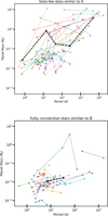 |
Fig. 10 Projected mass and orbital period of multiple systems around stars similar to 55 Cnc A (top) and 55 Cnc B (bottom). Symbols for the same system are connected by a line. The dashed black lines show the confirmed planets of 55 Cnc stars. Data are obtained from the Exoplanet Encyclopedia8. |
7 Conclusion
We conducted a comprehensive analysis of the 55 Cnc system, which was previously known to consist of two stars and five planets. We used the data acquired with CFHT/SPIRou over several years and studied both the RV and the circular polarisation in the stellar lines for both stars.
The magnetic properties of the primary. The primary star is an old Sun analogue and has a rotation period of 39 ± 1 days. The magnetic signal of 55 Cnc A dropped in amplitude in the early 2020s due to the expected cycle minimum. This contrasts with a previous campaign carried out during the cycle maximum in 2017, which recorded amplitudes approximately 10 times larger. We may expect the star to invert its polarity near the next maximum of the cycle in 2029 if its behaviour is solar-like (Charbonneau 2020). The updated cycle length is ∼4000 days or 10.96 years, coincidentally close to the solar cycle. A tenfold increase in the large-scale field amplitude results in a corresponding increase in stellar wind intensity and mass loss. Magneto-hydro-dynamical simulations of space weather around 55 Cnc A were conducted by Folsom et al. (2020) at cycle maximum, and their outputs can be scaled down by typically an order of magnitude at cycle minimum. Moreover, the small-scale magnetic field of the star during the SPIRou campaign, at minimum, is on average 250 ± 20 G.
The magnetic properties of the secondary. The rotational period of 55 Cnc B was estimated to be 92 ± 5 d from modulations of the differential temperature in the SPIRou data. Observed for the first time in high-resolution spectropolarimetry, the magnetic field of the secondary 55 Cnc B appears to be weak compared to other slowly rotating low-mass stars (e.g. Lehmann et al. 2024). It is characterised by a small-scale unsigned amplitude less than 60 G and a large-scale amplitude less than 10 G (3σ upper limit). With no detection in the nIR, it was not possible to find any modulation or derive its most probable topology. These upper limits support the presence of a quiet stellar surface, which is favourable for exoplanet searches using the RV method.
The exoplanet system around 55 Cnc A. The four inner planets (periods from 0.73 to 260 days) are confirmed, and their parameters are reassessed by this analysis. The errors on their orbital parameters have improved with the addition of new data. In particular, the eccentricity of the inner planet b is found to be smaller than previously reported (Nelson et al. 2014; Bourrier et al. 2018) and is consistent with 0 within the 1.1σ range. This new value supports the tidally damped dynamics of the orbit, characterised by rapid circularisation and the absence of a 3:2 spin-orbit resonance, as discussed in Ferraz-Mello & Beaugé (2025).
There is greater ambiguity regarding the outer system of this star. The period of the giant planet is now best modelled with an orbital period of 4800 days and a mass of 3.8 MJup. This orbit is only slightly eccentric or compatible with the circular one (eccentricity of 0.09 ± 0.07). Another signal at 3827 ± 9 days is also seen with an RV semi-amplitude of 13.1 ± 0.5 m/s. This signal is in phase with the magnetic cycle, as observed in the S index, at least during the first recorded cycle between 1994 and 2017. There are indications that the RV signal at this period is less in phase with the S index over the last decade, and also that the amplitude of this signal may be too large to be attributed to magnetic activity. In addition, the amplitude is not chromatic, and the star is extremely quiet. It is therefore possible that part of the RV signal at a 4000 d period (typically a few meters per second) is due to both the cycle and an outer planet intertwinned at a similar period. In the Solar System, the Jupiter orbit (4330 days) and the solar cycle (4015 days) are also coincidentally very close. Only additional data – both optical and nIR – and spectropolarimetry will allow us to disentangle RV magnetic cycle signatures as well as potential planetary signals in the long term. The potential confirmation of a second outer planet will require performing in-depth dynamical stability analyses, as strong interactions with the massive outer planet are expected. Moreover, it remains possible that the best-fit orbital periods of these outer planets evolve with additional data, as seen previously for planet d.
Spectropolarimetry in both optical and nIR spectral domains would be interesting to compare, as the physical processes responsible for the cycle may have different chromatic behaviour in both amplitude and scatter. This has never been studied in any star, not even in the Sun. This combined optical-nIR analysis will soon be possible with instruments such as VISION at the Télescope Bernard Lyot and Wenaokeao at CFHT, which will preserve the polarimetric information while giving simultaneous access to the relative spectrographs covering 370 to 2450 nm in one shot.
The first planets around 55 Cnc B. The presence of exoplanets around the secondary component was expected for several reasons: 1) common formation conditions with the primary, 2) the system’s metal-rich composition (although B is less metal-rich than A), and 3) the general tendency of low-mass stars forming with several low-mass planets (e.g. Dressing & Charbonneau 2015; Burn et al. 2021). However, due to its fainter luminosity, finding these planets with the RV method requires long exposures in the optical or the use of nIR spectrographs. SPIRou is well-suited for observing such stars and successfully detected two initial signals that we interpret as caused by exoplanets, based on 69 epochs of RV measurements. The most prominent short-period planet in the system has a 6.8 d period and a minimum mass of 3.5 M⊕. It is located at a semi-major axis of 0.044 ± 0.001 au and is currently best modelled with a circular orbit. The second planet is characterised by a larger minimum mass (5.3 M⊕) and an orbital period that is about five times longer. This pair of planets has a 5:1 period ratio, leaving room for additional low-mass planets in the system. More data would help strengthen the detection of the 33.7 d signal of 55 Cnc B, as this signal is detected at only 3.7σ given the current data. However, the presence of giant planets in the 55 Cnc B system is excluded by the data at this stage up to orbital periods of a couple of years. The ‘small sister’ of 55 Cnc A has its own planetary system, characterised by a more modest size and total mass than its primary.
Data availability
Full Tables A.1–A.3 are available at the CDS via https://cdsarc.cds.unistra.fr/viz-bin/cat/J/A+A/705/A190.
Acknowledgements
We are grateful to the referee for the careful reading and insightful suggestions that greatly improved the manuscript. This project received funding from the European Research Council under the H2020 research & innovation program (grant 740651 NewWorlds). We acknowledge the funding from Agence Nationale pour la Recherche (ANR, project ANR-18-CE31-0019 SPlaSH) and from the Investissements d’Avenir program (ANR-15-IDEX-02), through the “Origin of Life” project of the Université Grenoble Alpes. This publication makes use of The Data & Analysis Center for Exoplanets (DACE), which is a facility based at the University of Geneva (CH) dedicated to extrasolar planets data visualisation, exchange and analysis. DACE is a platform of the Swiss National Centre of Competence in Research (NCCR) PlanetS, federating the Swiss expertise in Exoplanet research. The DACE platform is available at https://dace.unige.ch. This research has made use of the SIMBAD database, operated at CDS, Strasbourg, France (Wenger et al. 2000). This work has made use of the VALD database, operated at Uppsala University, the Institute of Astronomy RAS in Moscow, and the University of Vienna.
References
- Artigau, É., Cadieux, C., Cook, N. J., et al. 2022, AJ, 164, 84 [NASA ADS] [CrossRef] [Google Scholar]
- Artigau, É., Cadieux, C., Cook, N. J., et al. 2024, AJ, 168, 252 [Google Scholar]
- Baluev, R. V. 2015, MNRAS, 446, 1493 [Google Scholar]
- Barnes, S. A. 2007, ApJ, 669, 1167 [Google Scholar]
- Boro Saikia, S., Jeffers, S. V., Morin, J., et al. 2016, A&A, 594, A29 [NASA ADS] [CrossRef] [EDP Sciences] [Google Scholar]
- Bourrier, V., Dumusque, X., Dorn, C., et al. 2018, A&A, 619, A1 [NASA ADS] [CrossRef] [EDP Sciences] [Google Scholar]
- Burn, R., Schlecker, M., Mordasini, C., et al. 2021, A&A, 656, A72 [NASA ADS] [CrossRef] [EDP Sciences] [Google Scholar]
- Butler, R. P., Marcy, G. W., Williams, E., Hauser, H., & Shirts, P. 1997, ApJ, 474, L115 [Google Scholar]
- Butler, R. P., Vogt, S. S., Laughlin, G., et al. 2017, AJ, 153, 208 [Google Scholar]
- Camacho, J. D., Faria, J. P., & Viana, P. T. P. 2023, MNRAS, 519, 5439 [NASA ADS] [CrossRef] [Google Scholar]
- Charbonneau, P. 2020, Liv. Rev. Sol. Phys., 17, 4 [Google Scholar]
- Cifuentes, C., Caballero, J. A., Cortés-Contreras, M., et al. 2020, A&A, 642, A115 [NASA ADS] [CrossRef] [EDP Sciences] [Google Scholar]
- Cook, N. J., Artigau, É., Doyon, R., et al. 2022, PASP, 134, 114509 [NASA ADS] [CrossRef] [Google Scholar]
- Crida, A., Ligi, R., Dorn, C., & Lebreton, Y. 2018, ApJ, 860, 122 [NASA ADS] [CrossRef] [Google Scholar]
- Cristofari, P. I., Donati, J. F., Folsom, C. P., et al. 2023a, MNRAS, 522, 1342 [NASA ADS] [CrossRef] [Google Scholar]
- Cristofari, P. I., Donati, J. F., Moutou, C., et al. 2023b, MNRAS, 526, 5648 [NASA ADS] [CrossRef] [Google Scholar]
- Dawson, R. I., & Fabrycky, D. C. 2010, ApJ, 722, 937 [Google Scholar]
- Delisle, J. B., Ségransan, D., Dumusque, X., et al. 2018, A&A, 614, A133 [NASA ADS] [CrossRef] [EDP Sciences] [Google Scholar]
- Díaz, R. F., Ségransan, D., Udry, S., et al. 2016, A&A, 585, A134 [Google Scholar]
- Donati, J. F., Semel, M., Carter, B. D., Rees, D. E., & Collier Cameron, A. 1997a, MNRAS, 291, 658 [Google Scholar]
- Donati, J. F., Semel, M., Carter, B. D., Rees, D. E., & Collier Cameron, A. 1997b, MNRAS, 291, 658 [Google Scholar]
- Donati, J. F., Howarth, I. D., Jardine, M. M., et al. 2006, MNRAS, 370, 629 [NASA ADS] [CrossRef] [Google Scholar]
- Donati, J. F., Kouach, D., Moutou, C., et al. 2020, MNRAS, 498, 5684 [Google Scholar]
- Donati, J. F., Cristofari, P. I., Finociety, B., et al. 2023, MNRAS, 525, 455 [NASA ADS] [CrossRef] [Google Scholar]
- Dressing, C. D., & Charbonneau, D. 2015, ApJ, 807, 45 [Google Scholar]
- Dumusque, X., Lovis, C., Ségransan, D., et al. 2011, A&A, 535, A55 [NASA ADS] [CrossRef] [EDP Sciences] [Google Scholar]
- Eggenberger, A., Udry, S., & Mayor, M. 2004, A&A, 417, 353 [NASA ADS] [CrossRef] [EDP Sciences] [Google Scholar]
- Endl, M., Robertson, P., Cochran, W. D., et al. 2012, ApJ, 759, 19 [Google Scholar]
- Ferraz-Mello, S., & Beaugé, C. 2025, A&A, 697, L8 [NASA ADS] [CrossRef] [EDP Sciences] [Google Scholar]
- Fischer, D. A. 2018, in Handbook of Exoplanets, ed. H. J. Deeg, & J. A. Belmonte, 3 [Google Scholar]
- Fischer, D. A., Marcy, G. W., Butler, R. P., et al. 2008, ApJ, 675, 790 [Google Scholar]
- Folsom, C. P., Bouvier, J., Petit, P., et al. 2018a, MNRAS, 474, 4956 [NASA ADS] [CrossRef] [Google Scholar]
- Folsom, C. P., Fossati, L., Wood, B. E., et al. 2018b, MNRAS, 481, 5286 [Google Scholar]
- Folsom, C. P., Ó Fionnagáin, D., Fossati, L., et al. 2020, A&A, 633, A48 [NASA ADS] [CrossRef] [EDP Sciences] [Google Scholar]
- Fulton, B. J., Petigura, E. A., Blunt, S., & Sinukoff, E. 2018, PASP, 130, 044504 [Google Scholar]
- Gaia Collaboration. 2020, VizieR Online Data Catalog, I/350 [Google Scholar]
- Gallet, F., & Bouvier, J. 2013, A&A, 556, A36 [NASA ADS] [CrossRef] [EDP Sciences] [Google Scholar]
- Gustafsson, B., Edvardsson, B., Eriksson, K., et al. 2008, A&A, 486, 951 [NASA ADS] [CrossRef] [EDP Sciences] [Google Scholar]
- Hara, N. C., Boué, G., Laskar, J., & Correia, A. C. M. 2017, MNRAS, 464, 1220 [Google Scholar]
- Haywood, R. D., Milbourne, T. W., Saar, S. H., et al. 2022, ApJ, 935, 6 [NASA ADS] [CrossRef] [Google Scholar]
- Hill, M. L., Bott, K., Dalba, P. A., et al. 2022, in LPI Contributions, 2687, Exoplanets in Our Backyard 2, 3046 [Google Scholar]
- Houdebine, E. R., Mullan, D. J., Paletou, F., & Gebran, M. 2016, ApJ, 822, 97 [NASA ADS] [CrossRef] [Google Scholar]
- Houdebine, É. R., Mullan, D. J., Doyle, J. G., et al. 2019, AJ, 158, 56 [NASA ADS] [CrossRef] [Google Scholar]
- Isaacson, H., Howard, A. W., Fulton, B., et al. 2024, ApJS, 274, 35 [NASA ADS] [CrossRef] [Google Scholar]
- Klein, B., Aigrain, S., Cretignier, M., et al. 2024, MNRAS, 531, 4238 [Google Scholar]
- Kochukhov, O., Makaganiuk, V., & Piskunov, N. 2010, A&A, 524, A5 [NASA ADS] [CrossRef] [EDP Sciences] [Google Scholar]
- Laliotis, K., Burt, J. A., Mamajek, E. E., et al. 2023, AJ, 165, 176 [NASA ADS] [CrossRef] [Google Scholar]
- Lehmann, L. T., Donati, J. F., Fouqué, P., et al. 2024, MNRAS, 527, 4330 [Google Scholar]
- Ligi, R., Creevey, O., Mourard, D., et al. 2016, A&A, 586, A94 [NASA ADS] [CrossRef] [EDP Sciences] [Google Scholar]
- Lovis, C., Dumusque, X., Santos, N. C., et al. 2011, arXiv e-prints [arXiv:1107.5325] [Google Scholar]
- Mann, A. W., Dupuy, T., Kraus, A. L., et al. 2019, ApJ, 871, 63 [Google Scholar]
- Marcy, G. W., Butler, R. P., Fischer, D. A., et al. 2002, ApJ, 581, 1375 [Google Scholar]
- Marfil, E., Tabernero, H. M., Montes, D., et al. 2021, A&A, 656, A162 [NASA ADS] [CrossRef] [EDP Sciences] [Google Scholar]
- McArthur, B. E., Endl, M., Cochran, W. D., et al. 2004, ApJ, 614, L81 [Google Scholar]
- Mengel, M. W., Fares, R., Marsden, S. C., et al. 2016, MNRAS, 459, 4325 [NASA ADS] [CrossRef] [Google Scholar]
- Meunier, N., & Lagrange, A. M. 2019, A&A, 628, A125 [NASA ADS] [CrossRef] [EDP Sciences] [Google Scholar]
- Meunier, N., Lagrange, A. M., & Desort, M. 2010, A&A, 519, A66 [NASA ADS] [CrossRef] [EDP Sciences] [Google Scholar]
- Meunier, N., Lagrange, A. M., Dumusque, X., & Sulis, S. 2024, A&A, 687, A303 [NASA ADS] [CrossRef] [EDP Sciences] [Google Scholar]
- Nelson, B. E., Ford, E. B., Wright, J. T., et al. 2014, MNRAS, 441, 442 [Google Scholar]
- Newton, E. R., Irwin, J., Charbonneau, D., et al. 2016, ApJ, 821, 93 [Google Scholar]
- Ould-Elhkim, M., Moutou, C., Donati, J. F., et al. 2023, A&A, 675, A187 [NASA ADS] [CrossRef] [EDP Sciences] [Google Scholar]
- Ould-Elhkim, M., Moutou, C., Donati, J. F., et al. 2025, A&A, 696, A152 [NASA ADS] [CrossRef] [EDP Sciences] [Google Scholar]
- Ould-Elhkim, M., Moutou, C., Donati, J.-F., et al. 2026, A&A, in press, https://doi.org/10.1051/0004-6361/202555469 [NASA ADS] [CrossRef] [EDP Sciences] [Google Scholar]
- Petit, P., Dintrans, B., Solanki, S. K., et al. 2008, MNRAS, 388, 80 [NASA ADS] [CrossRef] [Google Scholar]
- Petit, P., Louge, T., Théado, S., et al. 2014, PASP, 126, 469 [NASA ADS] [CrossRef] [Google Scholar]
- Petit, P., Böhm, T., Folsom, C. P., Lignières, F., & Cang, T. 2022, A&A, 666, A20 [NASA ADS] [CrossRef] [EDP Sciences] [Google Scholar]
- Rees, D. E., & Semel, M. D. 1979, A&A, 74, 1 [NASA ADS] [Google Scholar]
- Ribas, I., Reiners, A., Zechmeister, M., et al. 2023, A&A, 670, A139 [NASA ADS] [CrossRef] [EDP Sciences] [Google Scholar]
- Rosenthal, L. J., Fulton, B. J., Hirsch, L. A., et al. 2021, ApJS, 255, 8 [NASA ADS] [CrossRef] [Google Scholar]
- Ryabchikova, T., Piskunov, N., Kurucz, R. L., et al. 2015, Phys. Scr, 90, 054005 [Google Scholar]
- Satyal, S., & Cuntz, M. 2019, PASJ, 71, 53 [Google Scholar]
- Semel, M. 1989, A&A, 225, 456 [NASA ADS] [Google Scholar]
- Soubiran, C., Creevey, O. L., Lagarde, N., et al. 2024, A&A, 682, A145 [NASA ADS] [CrossRef] [EDP Sciences] [Google Scholar]
- Stassun, K. G., Oelkers, R. J., Paegert, M., et al. 2019, AJ, 158, 138 [Google Scholar]
- Thebault, P., & Bonanni, D. 2025, A&A, 700, A106 [NASA ADS] [CrossRef] [EDP Sciences] [Google Scholar]
- Thebault, P. & Haghighipour, N. 2015, in Planetary Exploration and Science: Recent Results and Advances, eds. S. Jin, N. Haghighipour, & W.-H. Ip, 309 [Google Scholar]
- Weiss, L. M., Marcy, G. W., Petigura, E. A., et al. 2018, AJ, 155, 48 [Google Scholar]
- Wenger, M., Ochsenbein, F., Egret, D., et al. 2000, A&AS, 143, 9 [NASA ADS] [Google Scholar]
- Winn, J. N., Matthews, J. M., Dawson, R. I., et al. 2011, ApJ, 737, L18 [Google Scholar]
- Zechmeister, M., & Kürster, M. 2009, A&A, 496, 577 [CrossRef] [EDP Sciences] [Google Scholar]
Values retrieved from the SIMBAD database are available at https://simbad.cds.unistra.fr/simbad
BF stands for the Bayes factor, defined as the differential Bayes information criterion in Ould-Elhkim et al. (2025)
The acronym FAP stands for the false alarm probability, which encodes the probability that a given peak in the periodogram is due to noise rather than a periodic signal.
The ∆AICc is the relative Akaike information criterion, defined in https://radvel.readthedocs.io/.
Information retrieved from the ‘planets in binaries’ database (Thebault & Bonanni 2025): https://exoplanet.eu/planets_binary/
Appendix A Table of data and parameters
SPIRou data of 55 Cnc A.
SPIRou data of 55 Cnc B.
PolarBase data of 55 Cnc A.
The full tables of SPIRou data are available in electronic format at CDS. Exerts are shown in Tables A.1 and A.2. Table A.3 lists the optical spectropolarimetric data found in Polarbase for 55 Cnc A, also available electronically in its full length.
Table C.1 lists the complete set of derived parameters for the planetary system of the primary star.
Appendix B Corner plots
In this Appendix, the corner plots of the fits computed in this article are shown. Figures C.1 and C.2 show the fundamental stellar parameters obtained from the SPIRou templates of 55 Cnc A and B, as modelled with Zeeturbo.
Figures C.3 and C.4 show the parameters of the time series of the differential effective temperature estimated in SPIRou spectra for 55 Cnc A and B, respectively.
Appendix C Full RV models
Figure C.6 shows all RV data used in the analysis of 55 Cnc A, with blue symbols for all optical data and red symbols for nIR SPIRou data. The raw RVs are shown in the top plot, the O-C residuals are shown in the middle plot after subtraction of 6 Keplerian signals, and the bottom plot shows the periodogram of the residuals with the modelled orbital periods and the rotation period.
Figure C.7 shows the full model for the RV time series of 55 Cnc B, including HIRES and CARMENES data (blue symbols) and SPIRou data used for the fit (red symbols). It also shows the residuals and its periodogram.
Finally, Figure C.5 shows the model parameters for the 55 Cnc B planetary system, assuming circular orbits.
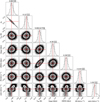 |
Fig. C.1 Posterior distribution of the fundamental parameters of 55 Cnc A as derived with SPIRou. Shown are the effective temperature, logg, [M/H], RV, vsini, and filling factors of the 0 and 2 kG surface small-scale magnetic field, a0 and a2. |
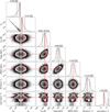 |
Fig. C.2 Same as Figure C.1, but for 55 Cnc B. |
Best-fit parameters of six Keplerian signals modelled in the time series of 55 Cnc A.
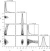 |
Fig. C.3 Corner plot of the quasi-periodic Gaussian process modelling for dTemp of 55 Cnc A. Shown are the amplitude of temperature variations in K (η1), the rotation period (η3), the smoothing parameter (η4), and the jitter. |
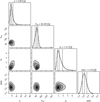 |
Fig. C.4 Same as Figure C.3, but for 55 Cnc B. |
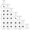 |
Fig. C.5 Corner plot of derived parameters of planets around 55 Cnc B. The orbits are assumed to be circular. |
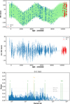 |
Fig. C.6 RadVel analysis of 55 Cnc A. Top: All instruments (optical instruments in blue, SPIRou in red) and all signals, as a function of time. Middle: O − C residuals. Bottom: GLS periodogram of residuals. |
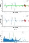 |
Fig. C.7 RadVel analysis of 55 Cnc B: Top: All instruments (HIRES and CARMENES in blue, SPIRou in red) and all signals, as a function of time. Middle: O − C residuals. Bottom: GLS periodogram of residuals. Top panel: Model calculated using SPIRou data only and overplotted over all data. |
All Tables
Best-fit parameters of six Keplerian signals modelled in the time series of 55 Cnc A.
All Figures
|
Fig. 1 Quasi-periodic GPR model of the differential temperature time series of 55 Cnc A (top) and B (bottom). |
| In the text | |
|
Fig. 2 Top: Time variations of the |
| In the text | |
|
Fig. 3 Magnetic geometry of 55 Cnc A. From left to right: ZDI models derived from observations from January to May 2023 (subset #1), September 2023 to May 2024 (subset #2), and October 2024 to February 2025 (subset #3). The stellar surface is shown in equatorial projection, with phases of observation indicated as vertical ticks above the top panel. The vector magnetic field is projected onto a spherical frame, with the radial, azimuthal, and meridional components displayed from top to bottom. The field strength is expressed in Gauss. |
| In the text | |
|
Fig. 4 Investigating magnetic field signatures for 55 Cnc B. Top: Intensity (Stokes I), null (Stokes N), and circularly polarised (Stokes V) profiles. Bottom: Variations of the longitudinal magnetic field as a function of time. |
| In the text | |
|
Fig. 5 RadVel analysis of 55 Cnc A. Shown are the individual signals, including the five planets. |
| In the text | |
|
Fig. 6 Top: residual RV signal of the sixth Keplerian as a function of time, with all other signals removed. The expected model for the magnetic cycle is superimposed in cyan (see text). Bottom: sixth Keplerian as a function of mean anomaly with the model in green. In both figures, the blue data correspond to all optical RV measurements, and the red data indicates SPIRou nIR RV measurements. |
| In the text | |
|
Fig. 7 ℓ1 periodogram of 55 Cnc B SPIRou RV data, showing prominent peaks at 6.8 and 33.7 d. |
| In the text | |
|
Fig. 8 Orbital solution obtained from SPIRou (‘s’) RV data of 55 Cnc B as a function of time (top) and phase (middle and bottom for planets b and c, respectively). The residuals are shown in panel b. Red points are mean measurements per regular 0.1 phase bins as calculated with RadVel when sufficient data is available. |
| In the text | |
|
Fig. 9 Planet-to-star mass ratio as a function of the orbital period for all known exoplanets. The planets orbiting both components of 55 Cnc are highlighted. The Symbol ‘Ag?’ corresponds to the maximum mass of a planet at a 3830 d period, if confirmed in the future. |
| In the text | |
|
Fig. 10 Projected mass and orbital period of multiple systems around stars similar to 55 Cnc A (top) and 55 Cnc B (bottom). Symbols for the same system are connected by a line. The dashed black lines show the confirmed planets of 55 Cnc stars. Data are obtained from the Exoplanet Encyclopedia8. |
| In the text | |
|
Fig. C.1 Posterior distribution of the fundamental parameters of 55 Cnc A as derived with SPIRou. Shown are the effective temperature, logg, [M/H], RV, vsini, and filling factors of the 0 and 2 kG surface small-scale magnetic field, a0 and a2. |
| In the text | |
|
Fig. C.2 Same as Figure C.1, but for 55 Cnc B. |
| In the text | |
|
Fig. C.3 Corner plot of the quasi-periodic Gaussian process modelling for dTemp of 55 Cnc A. Shown are the amplitude of temperature variations in K (η1), the rotation period (η3), the smoothing parameter (η4), and the jitter. |
| In the text | |
|
Fig. C.4 Same as Figure C.3, but for 55 Cnc B. |
| In the text | |
|
Fig. C.5 Corner plot of derived parameters of planets around 55 Cnc B. The orbits are assumed to be circular. |
| In the text | |
|
Fig. C.6 RadVel analysis of 55 Cnc A. Top: All instruments (optical instruments in blue, SPIRou in red) and all signals, as a function of time. Middle: O − C residuals. Bottom: GLS periodogram of residuals. |
| In the text | |
|
Fig. C.7 RadVel analysis of 55 Cnc B: Top: All instruments (HIRES and CARMENES in blue, SPIRou in red) and all signals, as a function of time. Middle: O − C residuals. Bottom: GLS periodogram of residuals. Top panel: Model calculated using SPIRou data only and overplotted over all data. |
| In the text | |
Current usage metrics show cumulative count of Article Views (full-text article views including HTML views, PDF and ePub downloads, according to the available data) and Abstracts Views on Vision4Press platform.
Data correspond to usage on the plateform after 2015. The current usage metrics is available 48-96 hours after online publication and is updated daily on week days.
Initial download of the metrics may take a while.