| Issue |
A&A
Volume 705, January 2026
|
|
|---|---|---|
| Article Number | A166 | |
| Number of page(s) | 12 | |
| Section | Astrophysical processes | |
| DOI | https://doi.org/10.1051/0004-6361/202556880 | |
| Published online | 16 January 2026 | |
Semi-analytic studies of the accretion disk and magnetic field geometry in M 87*
1
Max-Planck-Institut für Radioastronomie Auf dem Hügel 69 D-53121 Bonn, Germany
2
Instituto de Astrofísica de Andalucía-CSIC Glorieta de la Astronomía s/n E-18008 Granada, Spain
3
Research Centre for Theoretical Physics and Astrophysics, Institute of Physics, Silesian University in Opava CZ-74601 Opava, Czech Republic
4
Center for Astrophysics | Harvard & Smithsonian 60 Garden Street Cambridge MA 02138, USA
★★ Corresponding authors: This email address is being protected from spambots. You need JavaScript enabled to view it.
; This email address is being protected from spambots. You need JavaScript enabled to view it.
Received:
15
August
2025
Accepted:
3
November
2025
Abstract
Context. Magnetic fields play a pivotal role in the dynamics of black hole accretion flows and in the formation of relativistic jets. Observations by the Event Horizon Telescope (EHT) provided unprecedented insights into accretion structures near black holes. Interpreting these observations requires a theoretical framework that links polarized emission to the underlying system properties and magnetic field geometries.
Aims. We investigated how the system properties, in particular, the magnetic field geometry in the region of the event horizon scale, affect the structure of the observable synchrotron emission in M 87*. Specifically, we characterized the sensitivity of observables used by the EHT to black hole spin, plasma dynamics, accretion disk thickness, and magnetic field geometry.
Methods. We adopted a semi-analytic radiatively inefficient accretion flow model in Kerr spacetime. We varied the magnetic field geometry, black hole spin, accretion disk dynamics, and geometric thickness of the disk. We performed general relativistic ray-tracing with a full polarized radiative transfer to obtain synthetic images of M 87*. We extracted EHT observables, such as disk diameter, asymmetry, and polarimetric metrics from synthetic models. We also considered a number of general relativistic magnetohydrodynamics simulations and compared them with the semi-analytical models.
Results. The effect of the disk thickness on the observables is limited. On the other hand, magnetic configurations dominated by the toroidal and poloidal fields can be distinguished reliably. The flow dynamics, in particular, radial inflow, also significantly affects the EHT observables.
Conclusions. The M 87* system is most consistent with a flow dominated by the poloidal magnetic field with partially radial inflow. While the spin remains elusive, moderate or high positive values are preferred.
Key words: accretion / accretion disks / black hole physics / gravitation / magnetic fields / polarization / radiative transfer
Member of the International Max Planck Research School (IMPRS) for Astronomy and Astrophysics at the Universities of Bonn and Cologne.
© The Authors 2026
 Open Access article, published by EDP Sciences, under the terms of the Creative Commons Attribution License (https://creativecommons.org/licenses/by/4.0), which permits unrestricted use, distribution, and reproduction in any medium, provided the original work is properly cited.
This article is published in open access under the Subscribe to Open model.
Open access funding provided by Max Planck Society.
1. Introduction
It is unclear how magnetic fields govern the behavior of matter near black holes (BHs), as is the role they play in the formation of powerful jets and accretion flows in these extreme environments. This question remains central to our understanding of BH astrophysics. The interplay between magnetic fields and accretion flows significantly affects the immediate vicinity of BHs and extends to broader implications for galaxy dynamics and the evolution of supermassive BHs in active galactic nuclei (AGN; Blandford & Znajek 1977; Fabian 2012). At the event horizon scale, magnetic fields are thought to be crucial for angular momentum transport and energy dissipation within accretion flows (Balbus & Hawley 1991), thereby affecting the accretion rate and playing a key role in launching and collimating relativistic jets (Kovalev et al. 2005; Beckwith et al. 2008). These processes can be modeled with the equations of magnetohydrodynamics (MHD; e.g., Gammie et al. 2003; McKinney et al. 2012), with the structure and evolution of magnetic fields being key to deciphering the observed properties of BH systems, including their polarized emission.
It was not until the recent radio observations of the centers of galaxies Messier 87 (M 87*) and the Milky Way, Sagittarius A* (Sgr A*), by the Event Horizon Telescope (EHT; EHTC 2019a,d, 2022a,b) and the near-infrared (NIR) observations by the GRAVITY instrument (GRAVITY Collaboration 2018) that new avenues were opened to probe horizon-scale properties of BHs. EHT observations of M 87* and Sgr A* revealed compact bright ring-like emission structures with substantial central brightness depression, providing compelling evidence for the existence of supermassive compact objects in their cores (EHTC 2019a, 2022a). Subsequent analyses of the EHT observations yielded further insights into the physics of these systems, particularly through the study of polarized emission structures. They constrained the magnetic field geometry in the core region (EHTC 2021a,b, 2024a,b). These observations revealed dynamically important magnetic fields that are expected to play a crucial role in launching and collimating relativistic jets.
In order to explain the observations and model the behavior of magnetized plasma in the strong gravitational field near BHs, general relativistic magnetohydrodynamics (GRMHD) simulations are employed (Gammie et al. 2003; McKinney & Gammie 2004). These simulations have become an indispensable tool for investigating the intricate interplay between magnetic fields (McKinney et al. 2012; Gold et al. 2017; Ripperda et al. 2022), accretion flows (Porth et al. 2019; Narayan et al. 2022), and spacetime geometry (Mizuno et al. 2018; Chatterjee et al. 2023), and their combined effects (EHTC 2019a; Chatterjee et al. 2020; Nathanail et al. 2022).
While GRMHD simulations offer the most physically self-consistent framework for studying BH accretion, the inference based on these models remains contentious (e.g., Gralla 2021; Wielgus 2021). Despite its successes as an effective model, the set of equations solved by GRMHD is inadequate to describe collisionless plasma, assuming highly uncertain initial conditions. Furthermore, most of the results are obtained within the ideal MHD framework, while the important role of nonideal MHD effects such as magnetic reconnection in turbulent accretion flows near the event horizon is recognized (e.g., Ripperda et al. 2022). Global stationary semi-analytic approaches offer a complementary perspective by enabling parametric studies of accretion flows and magnetic field geometries. They allow us to investigate the effect of the prescribed disk properties and magnetic field geometry on the observable properties, including polarization of the emitted radiation (Narayan & Yi 1995; Pu & Broderick 2018). This approach constitutes a bridge between toy models that are useful for building intuition (e.g., Narayan et al. 2021) and computationally exhaustive GRMHD, where the parameters of the accretion disk and magnetic field follow the evolution of the MHD equations and cannot be modified explicitly.
A low-luminosity AGN system of M 87* falls into the category of radiatively inefficient accretion flows (RIAFs; Yuan et al. 2003) with a geometrically thick and optically thin accretion disk. Unlike optically thick and geometrically thin disks (Shakura & Sunyaev 1973), which efficiently cool down by blackbody radiation, RIAFs are characterized by low number densities and an extremely high temperature of ions that is decoupled from that of the radiating electrons. Thus, radiative cooling is inefficient, and excess energy is removed from the system through advection. A stationary semi-analytic RIAF model framework for M 87* was proposed (e.g., Broderick & Loeb 2009; Vincent et al. 2021). We systematically study the effect of the magnetic field configuration, BH spin, as well as geometric thickness and dynamics of the accretion disk on the observational appearance of RIAF models. We compare the RIAF results with GRMHD simulations, as well as with the characteristic observables extracted from the EHT data, including polarimetric quantities.
2. Model images of a black hole
We set up a stationary axisymmetric RIAF model in Kerr spacetime and subsequently performed numerical general relativistic ray-tracing using the open-source code ipole1 (Mościbrodzka & Gammie 2018). We assumed that the observed emission originates near the equatorial plane in the accretion flow, and we thus neglected potential contributions from the jet base. While the jet plays a major role for the source morphology and its energetic output at lower radio frequencies (e.g., Walker et al. 2018), the compact ring-like morphology of the 230 GHz EHT images of M 87* was found to be more consistent with the emission dominated by the accretion flow (e.g., EHTC 2019e, 2021b; Emami et al. 2023). This is particularly true for the favored strongly magnetized models (see EHTC 2019e and Sect. 2.4). While the extended jet in M 87* has been detected at 230 GHz (Goddi et al. 2021), observations support its subdominant role on compact scales at this frequency. The emission component corresponding to the jet on scales of ∼100 Schwarzschild radii has been weakly constrained only most recently in the EHT datasets (EHTC 2025a; Saurabh et al. 2025). Nonetheless, even if the emission is dominated by the accretion disk, the foreground jet may still act as a Faraday screen, modifying some polarimetric observables (Goddi et al. 2021; Wielgus et al. 2024). To capture these effects in the semi-analytic framework, a more complicated two-component disk + jet model would be necessary (see, e.g., preliminary work of Vincent et al. 2019). We provide relevant details of the disk model we used below.
2.1. RIAF setup
We adopted a simple semi-analytic RIAF model of a radiatively inefficient accretion flow (e.g., Broderick et al. 2016; Pu & Broderick 2018; Vos et al. 2022). In this framework, we prescribed a stationary model of the accretion flow instead of evolving conservative MHD equations. In particular, we assumed that the number density of electrons ne and electron temperature Te behaves as power laws of the spherical radius,
![Mathematical equation: $$ \begin{aligned} n_{\rm e}&= n_{\rm e,0} \left( \frac{r}{r_g} \right)^{-\delta } \exp \left[- \frac{1}{2} (H \tan \theta )^{-2} \right], \end{aligned} $$](/articles/aa/full_html/2026/01/aa56880-25/aa56880-25-eq1.gif) (1)
(1)
 (2)
(2)
for a gravitational radius rg = GMBH/c2, and we used the standard Boyer-Lindquist coordinate system (t, r, θ, ϕ) in Kerr spacetime of a rotating BH, parameterized with a spin (angular momentum) parameter a (Kerr 1963). We also defined a dimensionless spin parameter a* = a/M. Parameter H (dimensionless as well) controls the geometric thickness of the disk (Pu & Broderick 2018; Vincent et al. 2022). We took H = 0.5 as a fiducial geometrically thick model and additionally tested H = 0.1 and H = 0.3. There are some observational handles on γ in RIAF sources based on radiative spectra (e.g., Broderick et al. 2011) and VLBI brightness temperatures (Wielgus et al. 2024) of Sgr A*, and we therefore adopted a value of γ = 0.84 for our fiducial model, which is consistent with observational constraints. Our choices for all fiducial model parameters are given in Table 1.
Fiducial accretion flow model parameters.
To model the four-velocity of the accretion flow, we followed Pu et al. (2016), Tiede et al. (2020), and many others and interpolated between Keplerian orbital motion and geodesic free fall, hence
 (3)
(3)
 (4)
(4)
where (uKr, ΩK) and (uffr, Ωff) represent the radial four-velocity component ur and angular velocity Ω = uϕ/ut for Keplerian and for free-fall motion with zero angular momentum, respectively. In the Keplerian case, fluid motion inside the innermost stable circular orbit (ISCO) is modeled as a radial inspiral, following from the conservation of the ISCO values of energy E = −ut and angular momentum L = uϕ. We set uθ = 0 and obtained ut from the four-velocity normalization. We assumed ur < 0, that is, we did not allow for outflows (hence, no emission from the jets). Under the assumed parameterization, Keplerian motion corresponds to (κff, κK) = (0, 1), and free fall corresponds to (κff, κK) = (1, 0). Fractional values of these parameters result in a mixed nongeodesic prescription that is more appropriate for a model of a realistic astrophysical flow in M 87*, where a sub-Keplerian azimuthal velocity profile and advection are expected (e.g., Takahashi & Mineshige 2011). We considered (κff, κK) = (0, 1), (1, 0) and (0.5, 0.5), with the latter used as the fiducial RIAF model.
2.2. Magnetic field geometry
We considered several geometries of the magnetic field, embedded in the accretion flow described in Sect. 2.1. These are typically defined through vector potential A, thus enforcing the vanishing divergence of the magnetic field ∇iBi = 0. In our convention, Latin indices correspond to three spatial dimensions, while Greek ones span over all four spacetime dimensions. We assumed axisymmetric configuration, with the only nonzero component Aϕ, that is, Ar = Aθ = 0. The frame–dragging effect twists magnetic field lines and inevitably induces an electric field. As shown by Komissarov (2004, 2022), this induced electric field cannot be completely screened in the vicinity of a rotating BH. In particular, it is unscreened within the ergosphere. This is a general feature of this class of semi-analytic models, and we only focused on the magnetic field effect on the observables here. We considered the following seven geometries, illustrated in Fig. 1:
-
Radial (split monopole, e.g., Blandford & Znajek 1977)
 (5)
(5) -
vertical (e.g., Vos et al. 2022)
 (6)
(6) -
dipole (McKinney & Blandford 2009)
 (7)
(7)where ℱ− = 1 − cosμθ, ℱ+ = 1 + cosμθ, ν = 3/4, μ = 4, and r0 = 4rg,
-
quadrupole (McKinney & Blandford 2009)
 (8)
(8) -
parabolic (e.g., Tchekhovskoy et al. 2010; Kološ et al. 2023)
 (9)
(9)where we set k = 0.75 and for k = 0, this expression reduces to the radial magnetic field (split monopole),
-
combined field (Kenzhebayeva et al. 2024). This solution combines two fundamental field configurations, namely the vertical homogeneous solution of Wald (1974) and the radial (split-monopole), resulting in a paraboloidal field that is a self-consistent solution to the Maxwell equations in Kerr spacetime,
 (10)
(10)where p0 is the ratio of the radial to vertical magnetic field components.
-
Finally, for a toroidal configuration, it is straightforward to directly define a divergence-free magnetic field as
 (11)
(11)where g is the Kerr metric determinant.
For the configurations defined with a vector potential, with Ar = Aθ = 0, the laboratory frame (static observer’s frame) magnetic field components can be defined simply as
 (12)
(12)
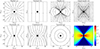 |
Fig. 1. Panels a–g: Schematic representation of the magnetic field configurations discussed in Sect. 2. Last panel: Example number density map for an RIAF model with a default disk thickness parameter H = 0.5. |
The asymptotic behavior of the magnetic field strength following these prescriptions is |B|∝r−1 for the vertical and toroidal configurations, |B|∝rk − 2 for the parabolic field, and |B|∝r−2 for the case of a radial field, dipole and quadrupole. The combined field asymptotes to a constant vertical magnetic field. Furthermore, the dipole field is predominantly vertical in the equatorial plane, and the quadrupole is predominantly radial in the equatorial plane, which is relevant for the signatures of a geometrically thin disk.
Subsequently, we normalized the magnetic fields by a constant factor, so that the magnetic field strength at the equatorial ring (r = 3rg, θ = π/2) was equal to B0 = 5 G, which is comparable to the EHT estimates (EHTC 2021b). In ideal magnetohydrodynamics the laboratory frame magnetic field Bμ is related to the fluid-frame magnetic field four-vector bμ as (Gammie et al. 2003)
 (13)
(13)
for the fluid four-velocity uμ, which we have defined in Sect. 2.1. The magnitude of bμ and its angle with respect to the momentum of the emitted photon kμ were then used to compute the intrinsic synchrotron emission, along with other radiative transfer parameters. While the magnetic fields that we defined are divergence-free by construction, we did not enforce the resulting configuration of (bμ, uμ) to be a stationary solution of the full induction equation in Kerr metric.
2.3. Emission and synthetic images
In order to perform the radiative transfer and ray-trace the synthetic images of the source, we followed the numerical setup described by Mościbrodzka & Gammie (2018). At radio frequencies, the emission from RIAF systems is dominated by the synchrotron radiation produced by hot electrons gyrating in the magnetic field (Yuan & Narayan 2014). We assumed a relativistic thermal (Maxwell-Jüttner) energy distribution of electrons and followed the fitting formulas of Pandya et al. (2016) to compute the necessary coefficients of the fully polarized radiative transfer, including emission, absorption, and Faraday effects.
For the mass and distance of M 87*, we assumed MBH = 6.4 × 10⁹ M⊙ and Ds = 16.9 Mpc, respectively (Gebhardt et al. 2011; EHTC 2019f, 2025b). We set the observing frequency to νobs = 230 GHz, which is within the observing frequency band of the EHT (EHTC 2019b,c). The inclination (viewing angle) with respect to the jet axis θi was estimated observationally (Mertens et al. 2016; Walker et al. 2018), with the ambiguity between θi and 180° −θi following from the overall symmetry of the system. The symmetry is broken by the orientation of the rotation, however. We adopted θi = 17° or θi = 163° = 180° −17°, assuming that the jet axis, angular momentum vector of the BH, and that of the accretion flow are all aligned along the same axis. The sign of the BH spin a* informs us whether the accretion flow and BH angular momenta are parallel (prograde rotation, a* > 0) or antiparallel (retrograde accretion, a* < 0). For our RIAF model, which lacks a jet, we identified θi with the angle calculated with respect to the angular momentum vector of the accretion disk rather than that calculated with respect to the angular momentum of the BH (which is either parallel or antiparallel). An additional prior comes from the EHT results EHTC (2019a), which constrain the brighter side of the observed ring to be located in the bottom side of the image. EHTC (2019e) argued that reproducing this orientation within the GRMHD library of images requires that the angular momentum vector of the BH is pointed away from the observer’s screen (see also comments in Sect. 4.2). Thus, we followed the convention of the EHT and took θi = 163° for the BH spins a* ≥ 0 and θi = 17° for a* < 0, which guarantees that the BH spin vector points away from the observer in all cases. Keeping θi = 163° for all BH spin values would result in a bright side of the ring flipped to the upper part of the image for a* < 0 GRMHD models, which is inconsistent with the EHT results.
We ray-traced images in the field of view (FOV) of 200 μas, corresponding to about 40 rg/Ds. The emission in the wider FOV in our idealized RIAF disk model is negligible, similarly as in the images reconstructed by the EHT (EHTC 2019d, 2024c). For each considered magnetic field model, accretion flow parameters κff, κK, and disk thickness parameter H, we tuned the number density scale ne, 0 and temperature scale Te, 0 to match the typically observed compact scale emission in M 87* of ℐtot = 0.5 Jy at 230 GHz (EHTC 2019d; Wielgus et al. 2020; EHTC 2024c) within 10% for the model with dimensionless spin a* = −0.94. We kept the same normalization for other spin values, which led to a flux density deviation from 0.5 Jy of up to a factor of 2. In all cases, our ne, 0 was within an order of magnitude from 104 cm−3, and Te, 0 was within an order of magnitude from 1011 K. This is reasonably consistent with the EHT estimates (EHTC 2021b).
2.4. GRMHD images
For comparison purposes, we also considered time-averaged GRMHD images from the EHT 230 GHz images library (EHTC 2021b; Wong et al. 2022; Dhruv et al. 2025). In these simulations, plasma and magnetic field co-evolve following the conservative MHD equations in a curved Kerr spacetime, reaching a quasi-stationary turbulent state of accretion. We considered ten simulations, computed for five different values of BH spin and for two different states of magnetization, a magnetically arrested disk (MAD), characterized by strong, coherent magnetic fields (Narayan et al. 2003), and a weak, turbulent magnetic field solution, “standard and normal evolution” (SANE; Narayan et al. 2012). Each of these two states predicts distinct dynamical outcomes and observable phenomena (Tchekhovskoy et al. 2011; Narayan et al. 2012). The models differ primarily in the strength and configuration of the magnetic fields threading the accretion flow, leading to distinct predictions for accretion rates, jet power, and observable emission characteristics. In the MAD regime, the magnetic flux threading the BH accumulates until it reaches a saturation point, which results in a magnetically dominated inner accretion flow. The accretion flow becomes highly nonaxisymmetric, with low-density magnetic flux bundles alternating with high-density streams of gas (Igumenshchev 2008), and the magnetic field lines exhibit a characteristic split-monopole configuration in the inner regions (Tchekhovskoy et al. 2011). In contrast, the SANE model represents a weakly magnetized accretion flow in which the accretion flow maintains a more axisymmetric structure than in MAD (Narayan et al. 2012). In this case, the magnetic field lines exhibit a more tangled and turbulent configuration (Sądowski et al. 2014). The location of the compact scale emission observed by the EHT in M 87* was discussed in EHTC (2019e). All MAD models considered in the EHT library were found to be dominated by the near-equatorial emission from the accretion flow. Emission from the jet base only manifests itself in some of the SANE models under assumptions resulting in a relatively low temperature of the electrons in the accretion disk.
For all models we considered, the electron energy distribution was relativistic thermal, which is a common assumption for modeling emission at frequencies νobs relevant for this work (EHTC 2019e). While the electron temperature Te in our RIAF models is governed by a radial power law given by Eq. (2), however, the GRMHD models prescribe Te as a function of the ion temperature Ti and the plasma βp parameter, a local ratio of gas pressure to magnetic pressure. These two quantities are constrained within a GRMHD simulation, and the local ion-to-electron temperature ratio is then evaluated as a postprocessing step with a parameter Rh, following Mościbrodzka et al. (2016)
 (14)
(14)
The results of EHTC (2019e, 2021b, 2023), and Joshi et al. (2024), where a range of values 1 ≤ Rh ≤ 160 were investigated, indicate a preference for a high value of Rh. In particular, most SANE models are inconsistent with a rather conservative lower limit on the observed jet power with only high negative BH spin or high positive BH spin, and Rh ≥ 80 surviving this constraint (EHTC 2019e). Hence, for comparisons with our RIAF models, we adopted a fixed value of Rh = 160, resulting in relatively cold electrons in the accretion disk region, and as a consequence, in stronger Faraday effects (Quataert & Gruzinov 2000) and associated depolarization EHTC (2021b, 2024b). Another consequence of larger Rh is that in order to reproduce the observed total intensity with colder electrons, a higher mass-accretion rate is required, which further increases the Faraday depth and generally enhances the jet power.
3. Method
To compare our synthetic images of the RIAF model and the EHT observations of M 87* (EHTC 2019a, 2021a), we defined quantifiable image metrics (not to be confused with the metric tensor) characterizing the source appearance in observations and in model images. We discuss the angular diameter of the ring and its brightness asymmetry as total intensity image metrics. Furthermore, we considered polarimetric consistency metrics following the method of EHTC (2021b). The summary of the EHT constraints for the image metrics we considered is given in Table 2.
EHT constraints on M 87* (EHTC 2019a, 2021a,b, 2024c).
3.1. Angular diameter of the ring
We extracted the size of the ring from the images using the REx module in the eht-imaging2 library (Chael et al. 2016), following the procedures of EHTC (2019d). The REx module allowed us to calculate the radial profiles of the intensity distribution, which can be used to determine the center and diameter of the ring. The diameter 𝒟 was estimated by the radial distance of the pixel with the peak intensity in the images. We blurred the synthetic RIAF images with a 15 μas circular Gaussian before extracting the profiles, in order to mimic the effective resolution of the EHT. Since the observable angular diameter scales with the uncertain mass over distance estimate θg = rg/Ds, equal to 3.74 μas for our fiducial parameters, we report the following normalized parameter (EHTC 2019f):
 (15)
(15)
The EHTC reported a measurement of parameter α for M 87* to be α = 11.0 ± 0.7, corresponding to a diameter of 42 ± 3 μas under the assumed rg/Ds (EHTC 2019a, 2024c). This is remarkably close to the theoretical prediction for the geometric BH shadow, in the sense of a trace of the photon shell (e.g., Bardeen et al. 1972) on the distant observer’s screen (the “apparent boundary” of Bardeen 1973 or the “critical curve” of Gralla et al. 2019). This prediction, which is dictated exclusively by GR through the null geodesic structure of spacetime, gives  for a Schwarzschild BH.
3.2. Brightness asymmetry
To quantify the brightness asymmetry in the total intensity image, we considered the ratio of the observed flux density between two halves of the image, separated by the line of the projected spin axis as indicated by Fig. 2,
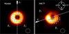 |
Fig. 2. Left: Example of an RIAF model with a* > 0 ray-traced at an inclination of 163°, blurred with a 15 μas circular Gaussian, indicated with a circle in the bottom right corner, before the 108° counterclockwise rotation to match it with the observed appearance of the M 87*. The ticks indicate the direction of polarization, vector a∗ shows the observer’s screen projection of the BH spin vector pointing away from the observer (into the screen). Right: Image of M 87* reconstructed from the EHT 2017 observations (EHTC 2019d). The axis shows the observed position angle of the jet, with the forward jet appearing toward the west at about 288° (Walker et al. 2018). The arrow shows the expected direction of the BH spin projection, pointing away from the observer. The 15 μas effective resolution of the image is indicated with a circle in the bottom right corner. Polarization ticks are shown in the region where ℐ > 0.1ℐmax and |

 (16)
(16)
We used REx in order to define the center of the ring. We used the position angle of the forward jet, constrained by the lower-frequency radio observations to be θPA = 288° (Walker et al. 2018), as a proxy for the BH spin axis (see Fig. 2 and comments in Sect. 2.3). We measured ℐr in the 2017 EHT images of M 87* (EHTC 2019d) to be 0.7±0.1 and in the 2018 EHT images of M 87* (EHTC 2024c) to be 0.6 ± 0.1, and we therefore took 0.65 ± 0.10 as the measurement of ℐr to be compared to the models.
3.3. Polarimetric observables
We followed EHTC (2021a,b) to define the metrics quantifying the polarization properties in the resolved and unresolved images. We denote the flux densities integrated over the field of view solid angle A as ℐtot for the total intensity,
 (17)
(17)
and 𝒫tot for the linear polarization,
 (18)
(18)
ℐtot and 𝒫tot are measured in jansky (Jy), while quantities with a tilde refer to the flux density per solid angle (brightness). ℐ, 𝒬, 𝒰, 𝒱 are the four Stokes parameters, describing the observed state of polarized emission. 𝒫tot is a complex number defining the strength and orientation of the polarized emission. The net polarization fraction, corresponding to a coherent average of  over the field of view and thus measurable from unresolved observations, is defined as
 (19)
(19)
For resolved EHT images, we also defined the incoherently averaged linear polarization fraction
 (20)
(20)
This metric depends on the effective image resolution, and following EHTC (2021a), we computed it on images blurred with a 15 μas circular Gaussian to mimic the effective EHT resolution. Furthermore, we considered the second mode of the azimuthal (in the ϕ angle direction) Fourier decomposition of the polarized image, denoted as β2 (Palumbo et al. 2020),
 (21)
(21)
The β2 metric exploits the approximate polar symmetry of the BH image observed at low inclination θi. The argument of this complex number characterizes the angle between the EVPA pattern and the BH image ring, while its absolute value informs us about how rotationally symmetric the EVPA pattern is.
4. Results
We present a grid of RIAF model images in Fig. 3. They were calculated for the fiducial parameters given in Table 1 and incorporate the various magnetic field geometries discussed in Sect. 2.2 and different values of the BH spin a*. All images exhibit a general ring morphology, with a prominent narrow photon ring (Johnson et al. 2020; Paugnat et al. 2022), formed by photons executing at least half loop around the BH on their way to the observer’s screen. The reconstructed EHT images, achieving an effective resolution of ∼15 μas, generally blend this feature with the diffused direct emission (see Fig. 2). The morphology of RIAF images is very similar to that found in time-averaged GRMHD images shown in Fig. 4. One outstanding feature is the second smaller ring that can be seen in SANE Rh = 160, a* = 0.94, which is the model for which the jet base emission dominates the disk emission (EHTC 2019e). A similar feature appears in the RIAF models for a dipole magnetic field configuration, where it is connected to the enhanced emission in the off-equatorial high-density region of magnetic field lines at intermediate values of θ (see panel (c) of Fig. 1). Another apparent feature in the GRMHD images is the depolarization of the northeast part of the ring seen in many of the images. This effect has been attributed to the Faraday rotation scrambling the polarization along light rays that spend a longer time in the accreting plasma (EHTC 2021b). The depolarization does not affect our fiducial RIAF images, which generally remain Faraday-thin. This is discussed further in Sect. 5.
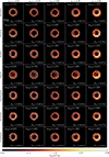 |
Fig. 3. Ray-traced images of the fiducial RIAF model (Table 1) with various magnetic field geometries and different BH spin a* values, shown in units of brightness temperature. The conventions for the inclination angle θi and the position angle θPA are described in Sect. 2.3. The total flux density ℐtot and the net fractional polarization |mnet| are indicated. The convention for showing EVPA ticks is the same as in Fig. 2. |
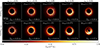 |
Fig. 4. Time-averaged ray traced GRMHD images from the EHT image library (EHTC 2019e, 2021b; Wong et al. 2022), representing different BH spin values a* and MAD or SANE states of magnetization. The conventions for the inclination angle θi and the position angle θPA are described in Sect. 2.3. The convention for showing EVPA ticks is the same as in Fig. 2. |
EHTC (2021b) and Narayan et al. (2021) discussed the relation between the magnetic field geometry and the observable EVPA pattern of the accretion system modeled as a thin emission ring. Following a simple argument of perpendicularity between polarization vector P, magnetic field B, and wave vector k for synchrotron emission, expressed with a P ∝ k × B relation, they concluded that toroidal magnetic fields produce a radial EVPA pattern and poloidal magnetic fields generally produce azimuthal EVPA patterns. With the images shown in Fig. 3, we confirm that these conclusions hold well for a more realistic spatially extended global emission models and geometries, as long as the Faraday depth is low.
4.1. Angular diameter of the ring
The ring size α parameter estimates for the fiducial velocity model are given in the left panel of Fig. 5. There is a small bias, with most models producing a slightly lower α than the observational constraints of the EHT. This can easily be explained through errors on the assumed a priori θg = rg/Ds, however, which are about 10%. The ring diameter depends weakly on the BH spin seen in the RIAF and in GRMHD simulations, with low spin models forming slightly larger rings. The effect is related to the BH event horizon and BH shadow, in the sense of a trace of the photon shell (e.g., Bardeen et al. 1972) on the distant observer’s screen (“apparent boundary” of Bardeen 1973 or the “critical curve” of Gralla et al. 2019) that decreases with the increase in |a*|.
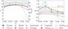 |
Fig. 5. Left: Diameter of the ring 𝒟 and normalized diameter α for the fiducial RIAF model with various magnetic field configurations and for GRMHD images as a function of BH spin a*. Right: Same for the brightness ratio parameter ℐr. The gray bands indicate constraints derived from the EHT observations of M 87*. |
It is notable that the sign of a* only plays a secondary role for the image size. The magnetic field configuration, on the other hand, does not significantly affect the measured diameter for the fiducial RIAF model. The high-spin SANE GRMHD model results in a significantly lower measurement of the diameter as a consequence of the jet base emission. This demonstrates that models dominated by jet emission are discouraged under rg/Ds priors and given the EHT observations (EHTC 2019e, 2021b, and Sect. 2 of this paper). Furthermore, in the first row of Fig. 7, we inspect the effect of the accretion flow velocity model on the normalized diameter α. While the fiducial sub-Keplerian and free-fall four-velocity models are close to the EHT constraints as well as to the GR predictions of the geometric BH shadow, Keplerian models with a high spin produce significantly smaller observable rings, with a size decreasing with a*. In these models, the accretion flow velocity remains purely azimuthal above the ISCO, while below the ISCO, the growing radial inflow velocity component in the plunging region results in beaming radiation toward the BH. This reduces the observed brightness and adds to the effects of gravitational redshift. Thus, most of the observed emission in the images of Keplerian models corresponds to the region close to ISCO. The ISCO radius is very sensitive to (signed) BH spin, changing from 9M for a* = −1 to 1M for a* = 1 (Bardeen et al. 1972). At the same time, the radius of the image of ISCO changes from about 10 θg to about 2 θg (see, e.g., Fig. 4 of Wielgus 2021). This means that for high positive BH spins, the primary image of ISCO manifests itself as a bright compact emission region contained within the geometric shadow (which itself is weakly dependent on spin). This biases the ring size measurements toward lower values. A similar behavior of Keplerian models has been reported by Vincent et al. (2022). As a consequence, high positive spin models can only be consistent with the θg prior for a non-Keplerian four-velocity, with significant inflow already above the ISCO. This effect underscores the importance of the astrophysical setup and that the measured ring diameter does not always approximately track the size of the geometric shadow (see also Gralla et al. 2019; Wielgus 2021; Urso et al. 2025). Finally, the geometric thickness of the disk does not affect the diameter strongly, as demonstrated in Fig. 8.
 |
Fig. 6. Variation in the net fractional polarization |m|net, resolved fractional polarization ⟨|m|⟩, amplitude and phase of the β2 parameter, and the net EVPA for the fiducial RIAF model with various magnetic field configurations and for GRMHD images as a function of BH spin a*. The gray bands indicate constraints derived from the EHT observations of M 87*. |
4.2. Brightness asymmetry
The emission forming the 230 GHz M 87* ring is expected to originate from the extremely compact region near the BH event horizon. The EHT observations and their interpretation confirm that most of the observed intensity originates at around 4–5 rg (EHTC 2019e). In this region, the effect of the BH spin on the photon trajectories is significant. Hence, the brightness asymmetry ℐr of the M 87* image essentially originates from the interplay of two effects: special relativistic Doppler boosting associated with the fluid motion, and general relativistic effects related to the BH spin. These effects deform the null geodesics and affect the length of the path that is within the emission region. EHTC (2019e) pointed out that for the GRMHD models in the EHT library, the BH spin position controls the direction of the image asymmetry, which is the origin of the convention for the image inclination dependent on the BH spin (see Sect. 2.3). Following this convention, if the ℐr estimates presented in the right panel of Fig. 5 are smaller than ℐr = 1, then the brighter side of the image is the bottom one (ℐ1 defined in Fig. 2). This is consistent with the EHT observations. In particular, for a negative BH spin, ℐr < 1 implies that the location of the brighter side is decided by the BH spin and is opposite to what would be observed if the BH did not spin (in which case, the Doppler boost would be the only cause of the brightness asymmetry). For most of our RIAF models, we found ℐr < 1 for a negative BH spin. Nonetheless, some Keplerian velocity models with negative BH spin indicate ℐr > 1 and might be brought into consistency with the observations by the image position angle rotation (see Fig. 7). The Keplerian models are also generally most asymmetric, and their brightness asymmetry is driven predominantly by the Doppler effect. Many of these Keplerian models can be rejected based on the excessive amount of asymmetry in comparison to the EHT images. On the other hand, far less asymmetry is observed in RIAF images corresponding to radial infall, for which no Doppler effect is associated with the azimuthal motion (Fig. 7). As a consequence, the zero angular momentum radial inflow RIAF models are too symmetric and thus inconsistent with the observations for all magnetic field configurations and all BH spins.
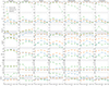 |
Fig. 7. Dependence of the image metrics discussed in Sect. 3 on the magnetic field geometry and BH spin a* for the fiducial RIAF model. Three models of plasma four-velocity pattern are considered (see Sect. 2.1). The gray bands indicate the constraints derived from the EHT observations of M 87*. |
With the exception of the negative spin MAD models, GRMHD images appear to be more asymmetric than the RIAF images with the fiducial sub-Keplerian velocity pattern (see Fig. 5). To obtain the amount of asymmetry similar to the positive spin GRMHD within RIAF framework, we require a more strongly azimuthal velocity pattern and a more azimuthally aligned velocity pattern in conjunction with a toroidal magnetic field (Fig. 7). A mixture of toroidal and poloidal magnetic fields is present in the GRMHD models, while the RIAF models we considered are either purely toroidal or purely poloidal.
The dependence of ℐr on the BH spin a* in Figs. 5–7 shows that the brightness asymmetry generally increases with growing positive spin because the Doppler and spin effects act in the same direction in this case. For a* < 0, the effects related to BH spin and the Doppler boosting act against one another and in most cases, produce a too symmetric image that is inconsistent with the observational constraints. Hence, the brightness asymmetry constrains the BH spin in a model-dependent way, with a preference toward high positive values of a* in fiducial RIAF models and moderate positive values for GRMHD. The models with a low negative BH spin are disfavored in both frameworks. Similarly as in case of the ring diameter, the accretion disk thickness H has a very limited effect on the brightness asymmetry (Fig. 8).
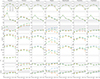 |
Fig. 8. Same as Fig. 7, but comparing three values of the geometric thickness H, as defined in Sect. 2.1. |
4.3. Polarimetric quantities
For a low inclination angle θi, a polarization pattern from an axisymmetric magnetic field averages out to a low value of |m|net. Many models, both GRMHD and RIAF, survive this observational constraint (see the first panel of Fig. 6). On the other hand, the resolved polarization fraction ⟨|m|⟩ is always too large in our RIAF models, significantly larger than observations and GRMHD models. Many SANE models are even too depolarized, and only some of the MAD models for low or mildly negative BH spin match the observational constraints. The reason for the large ⟨|m|⟩ in our RIAF models is likely the low contribution from Faraday effects, which causes significant depolarization in GRMHD models (particularly for a high assumed value of Rh) and, presumably, in the EHT observations (EHTC 2021b). For similar physical reasons, the absolute value of β2 is high for the circularly symmetric patterns in RIAF models, but much lower in GRMHD images as well as in the EHT observations. Keplerian models generally produce the least symmetric images (Sect. 4.2) and yield the lowest |β2|. Nonetheless, the argument of β2 appears to be a powerful test of the magnetic field geometry, particularly for a distinction between the dominance of the azimuthal magnetic field component, yielding argβ2 ≈ 0°, and various poloidal magnetic field configurations, for which argβ2 ≈ 180°. These findings also agree with the results obtained by Emami et al. (2023). GRMHD models reach values in between, which is expected from a mixed magnetic field configuration (see the fourth panel of Fig. 6). Keplerian RIAF models with poloidal magnetic fields exhibit a somewhat similar behavior (Fig. 7). Unlike GRMHD, these RIAF models do not obey the fluid four-velocity and magnetic field relation, constrained by the ideal MHD induction equation. The observed β2 angle is also in the intermediate range ( − 163° , − 127° ), indicating either a mixed magnetic field geometry or an impact from Faraday rotation. For vertical magnetic field configurations, we recovered the trends discussed by Palumbo (2025) and proposed as a test of a BH spin. While the trends are there, however, the values obtained with a global RIAF model differ from the predictions of a thin ring model used by Palumbo (2025), and a different magnetic field configuration may shift the values further or even reverse the trend direction. Finally, net EVPA, another quantity sensitive to the magnetic field geometry, was only weakly constrained by EHTC (2021a), but broadly corresponds to the direction parallel to the jet (θPA = −72°). We reproduced the observed EVPA with a number of RIAF models of various magnetic field configurations. The GRMHD models we considered, however, produce small positive net EVPA and are inconsistent with the observations. In a very simplistic (although commonly used) framework, vertical magnetic fields (parallel to the jet axis) would produce a perpendicular net EVPA at about 18°, while azimuthal magnetic fields (perpendicular to the jet axis) would produce a net EVPA around –72°. This heuristic works reasonably well for infalling and sub-Keplerian RIAF models with an azimuthal or vertical magnetic field structure (last panel of Fig. 6), but the higher azimuthal velocity and more complicated magnetic field structure affect this simple picture in a nontrivial way, however (last row of Fig. 7). Furthermore, we ignored the potential effect of Faraday rotation. For the M 87* rotation measure ∼105 rad m−2 (Goddi et al. 2021), the argument of β2 can be affected by up to about 20° and EVPA by up to about 10°.
4.4. Effect of the geometric disk thickness
The RIAF flows are expected to be very hot, and as a consequence, to be geometrically thick. Models often make a simplifying assumption of equatorial emission (e.g., Gralla et al. 2019; Paugnat et al. 2022; Urso et al. 2025). We tested the effect of geometric thickness on a number of observables. We summarize the results in Fig. 8. In most cases, the geometric thickness does not affect the results significantly. Hence, as long as the disk (and not the off-equatorial jet base) dominates the emission, the equatorial emission assumption provides a reasonable approximation of a more realistic thick disk. One exception is the dipolar magnetic field configuration, for which the geometrically thin disk is mostly threaded by a vertical magnetic field, but as the thickness increases, the emission region extends more into the off-equatorial radial magnetic field region (see Fig. 1). The effect is particularly strong for polarimetric observables, which are more sensitive to the magnetic field geometry.
5. Discussion and conclusions
We used a semi-analytic geometric RIAF disk model of BH accretion to study the effect of the system parameters on the seven observables, polarimetric ones in particular, that are used for evaluating theoretical models of M 87* (EHTC 2019e, 2021b). We considered five values of BH spin, seven distinct models of magnetic field geometry, three models of the plasma velocity pattern, and three values of the geometric thickness of the accretion flow. We compared our ray-traced synthetic images with the EHT observations as well as with a subset of GRMHD simulations from the EHT M 87* library computed at the observing frequency of 230 GHz.
We aimed to verify the simplifying assumptions that matter for the observables, and to which degree results obtained under simplifying assumptions can be interpreted quantitatively. We observed that the heuristic of radial polarization pattern implying azimuthal magnetic field structure and azimuthal polarization pattern implying poloidal magnetic fields generally holds for global accretion models, particularly for flows with non-negligible inflow, as expected in RIAFs. The geometric thickness of the disk does not affect the observables significantly in most cases, which might be an argument for the validity of conclusions obtained with a simplifying assumption of the equatorial emission. On the other hand, magnetic field geometry, plasma velocity profile, and BH spin all leave a strong imprint on the resulting images.
While we adjusted parameters to match the observed M 87* flux density of ∼0.5 Jy, our models remained Faraday thin, which is not the case for GRMHD simulations. The observations also indicate an appreciable Faraday depth through partial depolarization (EHTC 2021a,b). We further inspected this discrepancy by comparing our RIAF model setup to the GRMHD results in the EHT library, discussed by Dhruv et al. (2025). We found significant differences between the assumed RIAF structure discussed in Sect. 2.1 and predictions of GRMHD, such as a much steeper decrease in the gas temperature with radius seen in GRMHD. As a consequence, lower temperatures of the electrons in the emitting region might be a reason for the more pronounced Faraday effects seen in GRMHD (Quataert & Gruzinov 2000). Attempts to reproduce the appreciable Faraday depth by roughly matching the RIAF model properties to those of the averaged GRMHD were unsuccessful, however, which led us to the tentative conclusion that either nonaxisymmetric turbulent flow structure or off-equatorial jet base region plasma cause the observed depolarization.
As a consequence of the lack of depolarization, our RIAF models are all very symmetric, resulting in a large amplitude of β2 and resolved polarization degree ⟨|m|⟩. This is inconsistent with the observations. There is a caveat, related to the fact that we did not explore the effect of the inclination angle. The uncertainties of the observational estimate of the inclination are not smaller than about 5° −10°, which leaves some space for the fine-tuning. A higher inclination would generally reduce the image symmetry, bringing measurements of |β2| down. For the other remaining observables, most of the RIAF models violate at least some of those. The argument of β2 appears to be particularly constraining. One model that fares reasonably well against these constraints is the sub-Keplerian flow with a dipolar magnetic field configuration and a spin of a* = 0.5. This solution visually disagrees with the EHT image reconstruction, however, with a presence of a second ring (see the discussion in Sect. 4). More broadly, our results (particularly the argument of β2) indicate dominance of poloidal magnetic fields in M 87*, and the relatively high image brightness asymmetry discourages zero or mildly negative BH spins. It is apparent that the EHT observations have a strong constraining power over the accretion models. The model that is most consistent with the data would necessarily combine poloidal and toroidal magnetic field components, as well as azimuthal and radial velocity patterns.
Our analysis demonstrated that the horizon-scale observables depend in a systematic and physically interpretable way on the magnetic field geometry, plasma velocity structure, and black hole spin. Our main conclusions are summarized below.
-
The magnetic field geometry (in particular the distinction between the poloidal and toroidal field) strongly affects the structure of the polarized image and the EVPA pattern.
-
The plasma velocity profile affects multiple image properties, most notably, the asymmetry (which is highest for the Keplerian model), but also the polarimetric observables.
-
The black hole spin predominantly affects the images by increasing the brightness asymmetry. There are spin-dependent trends in the EVPA structure, but the effects are degenerate with respect to the magnetic field geometry and the velocity profile.
-
The geometric thickness plays a secondary role under the assumption that the emission is dominated by the accretion disk.
We discussed the effect of RIAF model parameters on the EHT observables mostly qualitatively. Some of the limitations of this work include fixed assumptions on the power-law structure of the flow and a lack of mixed toroidal-poloidal magnetic field configurations. Fitting a more general RIAF model directly to the EHT data would constitute an interesting follow-up work. The feasibility of a similar approach was recently demonstrated by SaraerToosi & Broderick (2025). Within the RIAF framework, accretion disk configurations in non-Kerr spacetimes might also be tested without resorting to computationally exhaustive covariant MHD numerical simulations (see Vincent et al. 2021 or the recent developments from Yin et al. 2025).
Acknowledgments
We thank George Wong for helpful comments as well as Frederic Vincent and the Paris Observatory in Meudon for hospitality during the work on this project. We thank Jack Livingston for internal refereeing of the manuscript. MW is supported by a Ramón y Cajal grant RYC2023-042988-I from the Spanish Ministry of Science and Innovation. Saurabh’s visit to Paris Observatory was supported by the Procope-Mobilität 2024 grant from the Embassy of France in Germany. This work was supported by the M2FINDERS project funded by the European Research Council (ERC) under the European Union’s Horizon 2020 Research and Innovation Programme (Grant Agreement No. 101018682). AT acknowledges the Alexander von Humboldt Foundation for its Fellowship and the Czech Science Foundation (GAČR) Grant No. 23-07043S. RE warmly acknowledges the generous support of the Institute for Theory and Computation (ITC) at the Center for Astrophysics.
References
- Balbus, S. A., & Hawley, J. F. 1991, ApJ, 376, 214 [Google Scholar]
- Bardeen, J. M. 1973, in Black Holes (Les Astres Occlus), eds. C. Dewitt, & B. S. Dewitt, 215 [Google Scholar]
- Bardeen, J. M., Press, W. H., & Teukolsky, S. A. 1972, ApJ, 178, 347 [Google Scholar]
- Beckwith, K., Hawley, J. F., & Krolik, J. H. 2008, ApJ, 678, 1180 [NASA ADS] [CrossRef] [Google Scholar]
- Blandford, R. D., & Znajek, R. L. 1977, MNRAS, 179, 433 [NASA ADS] [CrossRef] [Google Scholar]
- Broderick, A. E., & Loeb, A. 2009, ApJ, 697, 1164 [NASA ADS] [CrossRef] [Google Scholar]
- Broderick, A. E., Fish, V. L., Doeleman, S. S., & Loeb, A. 2011, ApJ, 735, 110 [NASA ADS] [CrossRef] [Google Scholar]
- Broderick, A. E., Fish, V. L., Johnson, M. D., et al. 2016, ApJ, 820, 137 [Google Scholar]
- Chael, A. A., Johnson, M. D., Narayan, R., et al. 2016, ApJ, 829, 11 [Google Scholar]
- Chatterjee, K., Younsi, Z., Liska, M., et al. 2020, MNRAS, 499, 362 [NASA ADS] [CrossRef] [Google Scholar]
- Chatterjee, K., Kocherlakota, P., Younsi, Z., & Narayan, R. 2023, arXiv e-prints [arXiv:2310.20040] [Google Scholar]
- Dhruv, V., Prather, B., Wong, G. N., & Gammie, C. F. 2025, ApJS, 277, 16 [Google Scholar]
- EHTC (Akiyama, K., et al.) 2019a, ApJ, 875, L1 [Google Scholar]
- EHTC (Akiyama, K., et al.) 2019b, ApJ, 875, L2 [Google Scholar]
- EHTC (Akiyama, K., et al.) 2019c, ApJ, 875, L3 [Google Scholar]
- EHTC (Akiyama, K., et al.) 2019d, ApJ, 875, L4 [Google Scholar]
- EHTC (Akiyama, K., et al.) 2019e, ApJ, 875, L5 [Google Scholar]
- EHTC (Akiyama, K., et al.) 2019f, ApJ, 875, L6 [Google Scholar]
- EHTC (Akiyama, K., et al.) 2021a, ApJ, 910, L12 [Google Scholar]
- EHTC (Akiyama, K., et al.) 2021b, ApJ, 910, L13 [Google Scholar]
- EHTC (Akiyama, K., et al.) 2022a, ApJ, 930, L12 [NASA ADS] [CrossRef] [Google Scholar]
- EHTC (Akiyama, K., et al.) 2022b, ApJ, 930, L14 [NASA ADS] [CrossRef] [Google Scholar]
- EHTC (Akiyama, K., et al.) 2023, ApJ, 957, L20 [NASA ADS] [CrossRef] [Google Scholar]
- EHTC (Akiyama, K., et al.) 2024a, ApJ, 964, L25 [NASA ADS] [CrossRef] [Google Scholar]
- EHTC (Akiyama, K., et al.) 2024b, ApJ, 964, L26 [CrossRef] [Google Scholar]
- EHTC (Akiyama, K., et al.) 2024c, A&A, 681, A79 [NASA ADS] [CrossRef] [EDP Sciences] [Google Scholar]
- EHTC (Akiyama, K., et al.) 2025a, A&A, 704, A91 [Google Scholar]
- EHTC (Akiyama, K., et al.) 2025b, A&A, 693, A265 [NASA ADS] [CrossRef] [EDP Sciences] [Google Scholar]
- Emami, R., Ricarte, A., Wong, G. N., et al. 2023, ApJ, 950, 38 [NASA ADS] [CrossRef] [Google Scholar]
- Fabian, A. C. 2012, ARA&A, 50, 455 [Google Scholar]
- Gammie, C. F., McKinney, J. C., & Tóth, G. 2003, ApJ, 589, 444 [Google Scholar]
- Gebhardt, K., Adams, J., Richstone, D., et al. 2011, ApJ, 729, 119 [Google Scholar]
- Goddi, C., Martí-Vidal, I., Messias, H., et al. 2021, ApJ, 910, L14 [NASA ADS] [CrossRef] [Google Scholar]
- Gold, R., McKinney, J. C., Johnson, M. D., & Doeleman, S. S. 2017, ApJ, 837, 180 [Google Scholar]
- Gralla, S. E. 2021, Phys. Rev. D, 103, 024023 [NASA ADS] [CrossRef] [Google Scholar]
- Gralla, S. E., Holz, D. E., & Wald, R. M. 2019, Phys. Rev. D, 100, 024018 [Google Scholar]
- GRAVITY Collaboration (Abuter, R., et al.) 2018, A&A, 615, L15 [NASA ADS] [CrossRef] [EDP Sciences] [Google Scholar]
- Igumenshchev, I. V. 2008, ApJ, 677, 317 [NASA ADS] [CrossRef] [Google Scholar]
- Johnson, M. D., Lupsasca, A., Strominger, A., et al. 2020, Sci. Adv., 6, eaaz1310 [NASA ADS] [CrossRef] [Google Scholar]
- Joshi, A. V., Prather, B. S., Chan, C.-K., Wielgus, M., & Gammie, C. F. 2024, ApJ, 972, 135 [Google Scholar]
- Kenzhebayeva, S., Toktarbay, S., Tursunov, A., & Kološ, M. 2024, Phys. Rev. D, 109, 063005 [Google Scholar]
- Kerr, R. P. 1963, Phys. Rev. Lett., 11, 237 [Google Scholar]
- Kološ, M., Shahzadi, M., & Tursunov, A. 2023, Eur. Phys. J. C, 83, 323 [Google Scholar]
- Komissarov, S. S. 2004, MNRAS, 350, 427 [Google Scholar]
- Komissarov, S. S. 2022, MNRAS, 512, 2798 [NASA ADS] [CrossRef] [Google Scholar]
- Kovalev, Y. Y., Kellermann, K. I., Lister, M. L., et al. 2005, AJ, 130, 2473 [Google Scholar]
- McKinney, J. C., & Blandford, R. D. 2009, MNRAS, 394, L126 [Google Scholar]
- McKinney, J. C., & Gammie, C. F. 2004, ApJ, 611, 977 [Google Scholar]
- McKinney, J. C., Tchekhovskoy, A., & Blandford, R. D. 2012, MNRAS, 423, 3083 [Google Scholar]
- Mertens, F., Lobanov, A. P., Walker, R. C., & Hardee, P. E. 2016, A&A, 595, A54 [NASA ADS] [CrossRef] [EDP Sciences] [Google Scholar]
- Mizuno, Y., Younsi, Z., Fromm, C. M., et al. 2018, Nat. Astron., 2, 585 [Google Scholar]
- Mościbrodzka, M., & Gammie, C. F. 2018, MNRAS, 475, 43 [CrossRef] [Google Scholar]
- Mościbrodzka, M., Falcke, H., & Shiokawa, H. 2016, A&A, 586, A38 [Google Scholar]
- Narayan, R., & Yi, I. 1995, ApJ, 452, 710 [NASA ADS] [CrossRef] [Google Scholar]
- Narayan, R., Igumenshchev, I. V., & Abramowicz, M. A. 2003, PASJ, 55, L69 [NASA ADS] [Google Scholar]
- Narayan, R., Sądowski, A., Penna, R. F., & Kulkarni, A. K. 2012, MNRAS, 426, 3241 [Google Scholar]
- Narayan, R., Palumbo, D. C. M., Johnson, M. D., et al. 2021, ApJ, 912, 35 [NASA ADS] [CrossRef] [Google Scholar]
- Narayan, R., Chael, A., Chatterjee, K., Ricarte, A., & Curd, B. 2022, MNRAS, 511, 3795 [NASA ADS] [CrossRef] [Google Scholar]
- Nathanail, A., Mpisketzis, V., Porth, O., Fromm, C. M., & Rezzolla, L. 2022, MNRAS, 513, 4267 [NASA ADS] [CrossRef] [Google Scholar]
- Palumbo, D. C. M. 2025, ApJ, 978, L4 [Google Scholar]
- Palumbo, D. C. M., Wong, G. N., & Prather, B. S. 2020, ApJ, 894, 156 [Google Scholar]
- Pandya, A., Zhang, Z., Chandra, M., & Gammie, C. F. 2016, ApJ, 822, 34 [Google Scholar]
- Paugnat, H., Lupsasca, A., Vincent, F. H., & Wielgus, M. 2022, A&A, 668, A11 [NASA ADS] [CrossRef] [EDP Sciences] [Google Scholar]
- Porth, O., Chatterjee, K., Narayan, R., et al. 2019, ApJS, 243, 26 [Google Scholar]
- Pu, H.-Y., & Broderick, A. E. 2018, ApJ, 863, 148 [NASA ADS] [CrossRef] [Google Scholar]
- Pu, H.-Y., Akiyama, K., & Asada, K. 2016, ApJ, 831, 4 [NASA ADS] [CrossRef] [Google Scholar]
- Quataert, E., & Gruzinov, A. 2000, ApJ, 545, 842 [NASA ADS] [CrossRef] [Google Scholar]
- Ripperda, B., Liska, M., Chatterjee, K., et al. 2022, ApJ, 924, L32 [NASA ADS] [CrossRef] [Google Scholar]
- Sądowski, A., Narayan, R., McKinney, J. C., & Tchekhovskoy, A. 2014, MNRAS, 439, 503 [CrossRef] [Google Scholar]
- SaraerToosi, A., & Broderick, A. 2025, ApJ, submitted [arXiv:2504.18624] [Google Scholar]
- Saurabh, Müller, H., von Fellenberg, S. D., et al. 2025, A&A, https://doi.org/10.1051/0004-6361/202557022 [Google Scholar]
- Shakura, N. I., & Sunyaev, R. A. 1973, A&A, 24, 337 [NASA ADS] [Google Scholar]
- Takahashi, R., & Mineshige, S. 2011, ApJ, 729, 86 [Google Scholar]
- Tchekhovskoy, A., Narayan, R., & McKinney, J. C. 2010, ApJ, 711, 50 [NASA ADS] [CrossRef] [Google Scholar]
- Tchekhovskoy, A., Narayan, R., & McKinney, J. C. 2011, MNRAS, 418, L79 [NASA ADS] [CrossRef] [Google Scholar]
- Tiede, P., Pu, H.-Y., Broderick, A. E., et al. 2020, ApJ, 892, 132 [NASA ADS] [CrossRef] [Google Scholar]
- Urso, I., Vincent, F. H., Wielgus, M., Paumard, T., & Perrin, G. 2025, A&A, 700, A193 [NASA ADS] [CrossRef] [EDP Sciences] [Google Scholar]
- Vincent, F. H., Abramowicz, M. A., Zdziarski, A. A., et al. 2019, A&A, 624, A52 [NASA ADS] [CrossRef] [EDP Sciences] [Google Scholar]
- Vincent, F. H., Wielgus, M., Abramowicz, M. A., et al. 2021, A&A, 646, A37 [NASA ADS] [CrossRef] [EDP Sciences] [Google Scholar]
- Vincent, F. H., Gralla, S. E., Lupsasca, A., & Wielgus, M. 2022, A&A, 667, A170 [NASA ADS] [CrossRef] [EDP Sciences] [Google Scholar]
- Vos, J., Mościbrodzka, M. A., & Wielgus, M. 2022, A&A, 668, A185 [NASA ADS] [CrossRef] [EDP Sciences] [Google Scholar]
- Wald, R. M. 1974, Phys. Rev. D, 10, 1680 [Google Scholar]
- Walker, R. C., Hardee, P. E., Davies, F. B., Ly, C., & Junor, W. 2018, ApJ, 855, 128 [Google Scholar]
- Wielgus, M. 2021, Phys. Rev. D, 104, 124058 [NASA ADS] [CrossRef] [Google Scholar]
- Wielgus, M., Akiyama, K., Blackburn, L., et al. 2020, ApJ, 901, 67 [Google Scholar]
- Wielgus, M., Issaoun, S., Martí-Vidal, I., et al. 2024, A&A, 682, A97 [NASA ADS] [CrossRef] [EDP Sciences] [Google Scholar]
- Wong, G. N., Prather, B. S., Dhruv, V., et al. 2022, ApJS, 259, 64 [NASA ADS] [CrossRef] [Google Scholar]
- Yin, H., Chen, S., & Jing, J. 2025, arXiv e-prints [arXiv:2507.03857] [Google Scholar]
- Yuan, F., & Narayan, R. 2014, ARA&A, 52, 529 [NASA ADS] [CrossRef] [Google Scholar]
- Yuan, F., Quataert, E., & Narayan, R. 2003, ApJ, 598, 301 [Google Scholar]
All Tables
All Figures
|
Fig. 1. Panels a–g: Schematic representation of the magnetic field configurations discussed in Sect. 2. Last panel: Example number density map for an RIAF model with a default disk thickness parameter H = 0.5. |
| In the text | |
|
Fig. 2. Left: Example of an RIAF model with a* > 0 ray-traced at an inclination of 163°, blurred with a 15 μas circular Gaussian, indicated with a circle in the bottom right corner, before the 108° counterclockwise rotation to match it with the observed appearance of the M 87*. The ticks indicate the direction of polarization, vector a∗ shows the observer’s screen projection of the BH spin vector pointing away from the observer (into the screen). Right: Image of M 87* reconstructed from the EHT 2017 observations (EHTC 2019d). The axis shows the observed position angle of the jet, with the forward jet appearing toward the west at about 288° (Walker et al. 2018). The arrow shows the expected direction of the BH spin projection, pointing away from the observer. The 15 μas effective resolution of the image is indicated with a circle in the bottom right corner. Polarization ticks are shown in the region where ℐ > 0.1ℐmax and |
| In the text | |
|
Fig. 3. Ray-traced images of the fiducial RIAF model (Table 1) with various magnetic field geometries and different BH spin a* values, shown in units of brightness temperature. The conventions for the inclination angle θi and the position angle θPA are described in Sect. 2.3. The total flux density ℐtot and the net fractional polarization |mnet| are indicated. The convention for showing EVPA ticks is the same as in Fig. 2. |
| In the text | |
|
Fig. 4. Time-averaged ray traced GRMHD images from the EHT image library (EHTC 2019e, 2021b; Wong et al. 2022), representing different BH spin values a* and MAD or SANE states of magnetization. The conventions for the inclination angle θi and the position angle θPA are described in Sect. 2.3. The convention for showing EVPA ticks is the same as in Fig. 2. |
| In the text | |
|
Fig. 5. Left: Diameter of the ring 𝒟 and normalized diameter α for the fiducial RIAF model with various magnetic field configurations and for GRMHD images as a function of BH spin a*. Right: Same for the brightness ratio parameter ℐr. The gray bands indicate constraints derived from the EHT observations of M 87*. |
| In the text | |
|
Fig. 6. Variation in the net fractional polarization |m|net, resolved fractional polarization ⟨|m|⟩, amplitude and phase of the β2 parameter, and the net EVPA for the fiducial RIAF model with various magnetic field configurations and for GRMHD images as a function of BH spin a*. The gray bands indicate constraints derived from the EHT observations of M 87*. |
| In the text | |
|
Fig. 7. Dependence of the image metrics discussed in Sect. 3 on the magnetic field geometry and BH spin a* for the fiducial RIAF model. Three models of plasma four-velocity pattern are considered (see Sect. 2.1). The gray bands indicate the constraints derived from the EHT observations of M 87*. |
| In the text | |
|
Fig. 8. Same as Fig. 7, but comparing three values of the geometric thickness H, as defined in Sect. 2.1. |
| In the text | |
Current usage metrics show cumulative count of Article Views (full-text article views including HTML views, PDF and ePub downloads, according to the available data) and Abstracts Views on Vision4Press platform.
Data correspond to usage on the plateform after 2015. The current usage metrics is available 48-96 hours after online publication and is updated daily on week days.
Initial download of the metrics may take a while.