| Issue |
A&A
Volume 705, January 2026
|
|
|---|---|---|
| Article Number | A31 | |
| Number of page(s) | 9 | |
| Section | Galactic structure, stellar clusters and populations | |
| DOI | https://doi.org/10.1051/0004-6361/202557112 | |
| Published online | 07 January 2026 | |
The chemical DNA of the Magellanic Clouds
IV. Unveiling extreme element production: The Eu abundance in the Small Magellanic Cloud★
1
Dipartimento di Fisica e Astronomia “Augusto Righi”, Alma Mater Studiorum, Università di Bologna,
Via Gobetti 93/2,
40129
Bologna,
Italy
2
INAF – Osservatorio di Astrofisica e Scienza dello Spazio di Bologna,
Via Gobetti 93/3,
40129
Bologna,
Italy
3
INAF – Osservatorio Astrofisico di Arcetri,
Largo E. Fermi 5,
50125,
Firenze,
Italy
★★ Corresponding author: This email address is being protected from spambots. You need JavaScript enabled to view it.
Received:
5
September
2025
Accepted:
8
November
2025
Abstract
In this study we investigate the chemical enrichment of the rapid neutron-capture process in the Small Magellanic Cloud (SMC). We measured the [Eu/Fe] abundance ratio of 209 giant stars that are confirmed members of the SMC, providing the first extensive dataset of Eu abundances in this galaxy across its full metallicity range, spanning more than 1.5 dex. We compared the Eu abundances with those of Mg and Ba to evaluate the efficiency of the r-process relative to α-capture and s-process nucleosynthesis. The SMC shows enhanced [Eu/Fe] values at all metallicities (comparable with the values measured in the Milky Way) and a clear decline as [Fe/H] increases (from approximately −1.75 dex to approximately −0.5 dex), which is consistent with the onset of Type Ia supernovae. In contrast, [Eu/Mg] is enhanced by about +0.5 dex at all [Fe/H] and thus significantly above the values observed in Milky Way stars, where [Eu/Mg] remains close to the solar value, reflecting comparable production of r-process and α-capture elements. Moreover, [Ba/Eu] increases with metallicity beginning at [Fe/H] ≈ −1.5 dex, namely at a lower metallicity with respect to the Milky Way, where [Ba/Eu] starts to increase around [Fe/H] ≈ −1 dex. Our findings suggest the SMC has a higher production of Eu (with respect to the α-elements) than the Milky Way, but it is still in line with what has been observed in other dwarf systems within the Local Group. We confirm that galaxies with star formation efficiencies lower than the Milky Way have a high [Eu/α], probably indicating stronger efficiency of the delayed sources of the r-process at low metallicities.
Key words: galaxies: abundances / Local Group / Magellanic Clouds
Based on observations collected at the ESO-VLT under the program 113.26EF.
© The Authors 2026
 Open Access article, published by EDP Sciences, under the terms of the Creative Commons Attribution License (https://creativecommons.org/licenses/by/4.0), which permits unrestricted use, distribution, and reproduction in any medium, provided the original work is properly cited.
This article is published in open access under the Subscribe to Open model. This email address is being protected from spambots. You need JavaScript enabled to view it. to support open access publication.
1 Introduction
Neutron-capture processes overcoming the high Coulomb barriers of high-Z nuclei are responsible for the formation of the majority of the elements heavier than the Fe-peak (see e.g. Burbidge et al. 1957). Depending on the balance between the timescales of the neutron captures and of the β-decay these elements are labelled as rapid (r), intermediate, or slow (s) neutron-capture elements. The r-process is the most extreme among these, requiring a neutron flux of the order of ∼1020 cm−3.
The astrophysical sites for the occurrence of the r-process are still debated. Our current view is that two concurrent production sites contribute to produce the r-process elements: (1) a prompt source occurring on timescales shorter than tens of megayears involving some peculiar core-collapse supernovae (SNe), such as the magneto-rotationally driven SNe (e.g. Winteler et al. 2012), the supernova-triggering collapse of rapidly rotating massive stars (collapsars, e.g. Siegel et al. 2019), or highly magnetised neutron stars (magnetars, e.g. Patel et al. 2025), and (2) a delayed source occurring on timescales up to a few gigayears identified in compact binary mergers (neutron star-neutron star or neutron star-black hole, hereafter just referred to as NSMs) corresponding to explosive kilonova events connected to the previous gravitational wave emission (Argast et al. 2004; Thielemann et al. 2017). The detection of electromagnetic radiation from the gravitational wave event GW170817 (Abbott et al. 2017) has provided direct evidence of the contribution of NSMs to r-process nucleosynthesis (see e.g. Pian et al. 2017; Watson et al. 2019). Chemical evolution models reproduce fairly well the abundance patterns of r-process elements measured in our Galaxy by means of the combined action of both prompt and delayed sources (e.g. Côté et al. 2019; Molero et al. 2023; Palla et al. 2025), further contributing to the idea of multiple sources acting on different timescales as r-process production sites.
Recently, the study of r-process elements has received considerable attention in the field of Galactic archaeology. In particular, Europium has garnered interest due to its very low ‘contamination, by s-process production since, in metal-poor stars, the Eu abundance pattern is consistent with a pure r-process origin (see e.g. Burris et al. 2000). In fact, the [Eu/a] abundance ratio can serve as a powerful diagnostic for distinguishing between in situ and accreted stellar populations in the Milky Way (MW) halo (Monty et al. 2024; Ernandes et al. 2024; Ceccarelli et al. 2024). Indeed, stars and globular clusters identified as being accreted based on their dynamical properties exhibit higher [Eu/a] ratios than in situ stars at metallicities above [Fe/H]~ −1.3 dex, which is precisely where the largest chemical differences between in situ and accreted populations are observed (see e.g. Nissen & Schuster 2010; Helmi et al. 2018; Matsuno et al. 2022; Ceccarelli et al. 2024). This suggests that the production of r-process elements may be higher when compared to that of α-elements (mostly taking place in massive stars ending their lives as core-collapse SNe, e.g. Arcones & Thielemann 2023) in stars formed in now-dissolved accreted systems, whose masses were comparable to those of present-day dwarf spheroidal (dSph) or ultra-faint dwarf galaxies.
This result is consistent with studies conducted over the past two decades on both isolated dwarf galaxies and those currently interacting with or merging into the MW. In such galaxies, [«/Fe] is typically lower than in the MW at similar [Fe/H], reflecting their lower star formation efficiency (see Matteucci 2021 and references therein), while [Eu/Fe] remains elevated, indicating strong r-process activity. Indeed, these patterns have been observed in the Large Magellanic Cloud (LMC, Mucciarelli et al. 2010; Van der Swaelmen et al. 2013), in Fornax (Letarte et al. 2010) and Sculptor dSphs (Hill et al. 2019), and in the remnant of the Sagittarius dSph (Sbordone et al. 2007; Reichert et al. 2020; Liberatori et al. 2025). These findings underscore the importance of tracing the chemical evolution of dwarf galaxies in order to interpret the properties of accreted stellar populations now residing in the Galactic halo.
Recently, Palla et al. (2025) addressed the problem of modelling the r-process enrichment in Local Group galaxies by including both prompt and delayed sources, as commonly assumed in the literature (e.g. Prantzos et al. 2020; Kobayashi et al. 2020; Molero et al. 2021). Their results showed that chemical prescriptions that are able to reproduce Eu abundance patterns in MW stars well fail to reproduce the abundances measured in dwarf galaxies, predicting too-low [Eu/Fe] and [Eu/α] ratios, while they are able to reproduce the measured [«/Fe]. To solve this missing Eu problem, the authors suggested an increased production from delayed sources at low metallicity, which provides a much better match to the observed trends in the MW and Local Group dwarf galaxies.
All of these observational and theoretical findings further underscore the need to investigate in even more detail r-process enrichment (and therefore Eu abundance patterns) in Local Group systems with stellar masses and star formation efficiencies lower than those of the MW. In this context, the Small Magellanic Cloud (SMC) has received very limited attention so far (Nidever et al. 2020; Mucciarelli et al. 2023a, hereafter Paper I), and information on the Eu abundances in its stellar populations remains scarce. Indeed, the only measurements of [Eu/Fe] are available for two very metal-poor SMC field stars (Reggiani et al. 2021) and for three globular clusters at higher metallicities (Mucciarelli et al. 2023b).
This work aims to fill this gap by providing, for the first time, a large dataset of Eu abundances derived from high-resolution spectra in order to investigate the efficiency of r-process enrichment in the SMC relative to α- and s-processes. The Eu abundances are also compared with those of other nucleosyn-thetic processes, such as the α-capture, here traced by Mg and occurring in massive stars, and the s-process, traced by Ba and occurring mostly in low- and intermediate-mass asymptotic giant branch (AGB) stars. In addition, Ba serves as a further indicator of the r-process efficiency at low-metallicity, as it receives significant contribution where s-process production is disfavoured (due to the metallicity dependence of the s-process, see e.g. Arcones & Thielemann 2023). In this way, the results presented here will not only provide new constraints on the chemical evolution of the SMC but also offer valuable insights into the role of r-process nucleosynthesis in low-mass, low-efficiency star-forming systems within the Local Group.
The paper is organised as follows. In Section 2, we summarise the observations and the dataset analysed in this study. In Section 3 we describe the methods used to infer atmospheric parameters, radial velocities, and chemical abundances of the target stars. Section 4 presents the results, and in Section 5 we discuss the interpretation of the measured abundance patterns. Finally, in Section 6, we draw our conclusions.
2 Observation and data reduction
This study is based on observations (Program ID: 113.26EF, PI: Mucciarelli) performed with the multi-object spectrograph FLAMES (Pasquini et al. 2002) targeting the same fields analysed in Paper I. We focus on three SMC fields - FLD-121, FLD-339, and FLD-419 - each centred on a globular cluster (NGC 121, NGC 339, and NGC 419, respectively; see Fig. 1 in Paper I). These three fields are located in different positions of the SMC in order to sample the chemical composition of the SMC close to the main body of the galaxy (FLD-339 and FLD-419) and its outskirts (FLD-121). The observations discussed in Paper I were based on the HR11 and HR13 FLAMES setups that do not include any Eu transition in their spectral range.
The new observations presented here were carried out with the HR15n FLAMES setup (R = 19 200, 6470 Å <λ< 6790 Å), sampling the Eu II line at 6645 Å. For each field, three exposures of 45 minutes each were secured in order to obtain, for the co-added spectra, a signal-to-noise ratio (S/N) of ∼50 and ∼100 for the faintest (G ∼ 16.6) and brightest (G ∼ 16) targets, respectively. A total of 209 giant star members of the SMC were observed. Of these, 158 are also in the sample of Paper I, while the other 51 targets are new and were selected from Gaia Data Release 3 photometry (Gaia Collaboration 2021). These new stars were selected in the magnitude range G ∼ 16-16.6 and we excluded objects with poor photometric quality (as traced by the Gaia parameter phot_bp_rp_excess_factor, Lindegren et al. 2018). This magnitude range allowed us to have stars with S/N larger than 50 (faint limit) and include only stars belonging to the red giant branch (RGB) older than ∼ 1Gyr (bright limit); thus, we excluded bright stars corresponding to younger populations. We also excluded stars with companions located within 2″ and brighter by ≤2 magnitudes in G compared to the target star in order to avoid fibre contamination from nearby sources.
The spectra analysed in this work were then reduced following the ESO FLAMES-GIRAFFE pipeline1. All the reduced spectra were cleaned of cosmic rays, corrected for the heliocentric velocity, co-added, and finally normalised. Table 1 lists the main information for all the spectroscopic targets, including the Gaia identification number, the coordinates, the G magnitude, the identification number used in Paper I for the stars in common, the field, and an indication of whether the target star is a likely binary system.
3 Spectral analysis
3.1 Radial velocities
Radial velocities (RVs) for all the new spectra were measured by exploiting the standard cross-correlation technique (see e.g. Tonry & Davis 1979) as implemented in the PyAstronomy package. Synthetic spectra computed with the SYNTHE code (Kurucz 2005), following the procedure described in Section 3.2, were adopted as templates. The HR15n FLAMES setup does not include any sky emission line that allows us to check the accuracy of the wavelength calibration. We compared the RVs of the stars in common with Paper I (where the zero-point of the wavelength calibration was checked using the O emission sky line at 6300 Å), finding a median difference of −1 km/s. We applied this offset to all the RVs derived from HR15n spectra. The new 51 target stars are all members of the SMC and they have RVs compatible with the RV distribution of the galaxy (see e.g. De Leo et al. 2020; Nidever et al. 2020, Paper I). The typical uncertainties of the heliocentric RVs are ≃0.1 km/s.
To check for possible binary stars, we compared the RVs derived in the two available epochs for the stars in common with Paper I (see Fig. 1). Most of the data cluster around zero, with some points appearing as clear outliers, with absolute RV differences exceeding 10 km/s. We performed an iterative 3σ rejection on this sub-sample. Convergence (i.e. no further values being excluded) was reached for a sub-sample of 149 stars, which can be considered as normally distributed. Nine stars were excluded as outliers and considered candidate binaries. The surviving sample has a mean RV of −0.09 km/s and a standard deviation of 1.51 km/s. This dispersion is not compatible with the RV measurement errors, suggesting that the spread is real and that it can be attributed to radial pulsations, which can cause RV variations on the order of 1-2 km/s in stars near the tip of the RGB (Carney et al. 2003; Hekker et al. 2008), such as those analysed in this study.
Information about the SMC spectroscopic targets.
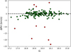 |
Fig. 1 Difference between the RVs derived in this study and those in Paper I as a function of the Gaia DR3 G magnitude. The red circles are stars with discrepant RV differences after a 3σ-clipping iterative procedure. |
3.2 Atmospheric parameters
The derived atmospheric parameters are listed in Table 2. For the stars in common with Paper I, we adopted the reported stellar parameters for these objects, namely, the effective temperatures (Teff), surface gravities (log g), and microturbulent velocities (vt). For the new targets, the stellar parameters were calculated from the photometry adopting the same approach used in Paper I. In particular, Teff were obtained from the broad-band colour (G – KS)0 using the (G – KS)0 – Teff transformation provided by Mucciarelli et al. (2021), and the values we calculated for Teff range from ∼3800 to ∼4500 K. We adopted G magnitudes from Gaia Data Release 3 (Gaia Collaboration 2021) and KS from 2MASS (Skrutskie et al. 2006). The G magnitudes were corrected for extinction following the prescriptions by Gaia Collaboration (2018), while for KS magnitudes, the extinction coefficient by McCall (2004) was adopted. The colour excess values, E(B-V), are from the infrared dust maps by Schlafly & Finkbeiner (2011).
Surface gravities were obtained from the Stefan-Boltzmann law, assuming Teff, a stellar mass equal to 1M⊙ and a true distance modulus DM0 = 18.965 ± 0.025 (Graczyk et al. 2014) and calculating the bolometric correction following Andrae et al. (2018). The assumption of 1 M⊙ is reasonable according to the age distribution of the SMC stars (see discussion in Paper I). While it is not possible to derive precise masses for individual targets, a variation of ±0.2 M⊙ from this assumed value results in a change in the log g smaller than 0.1 dex, with a negligible impact on the derived abundances. When considering the distance modulus, it should be noted that the SMC is characterised by a significant line-of-sight depth that it is not easy to properly evaluate for each single target. The depth maps provided by Subramanian & Subramaniam (2009) indicate that the three target fields discussed here should cover a depth range between 2 and 6 kpc. When a conservative distance variation of 3 kpc is assumed, the uncertainties in log g only increase by 0.02 dex, translating into variations of less than 0.02 in the abundances of single ionised lines (such as Ba and Eu lines). The final error in log g is then dominated by the uncertainties in the stellar mass. The values we calculated for log g range from 0.4 to 1.1 (in cgs units).
The microturbulent velocity vt is usually derived spectroscopically by removing any trend between the iron abundance and the strength of the lines (see Mucciarelli 2011, for a review of this approach). Our spectra have a relatively small number (∼30) of FeI lines, so the spectroscopic determination of vt could be affected by statistical fluctuations, thus leading to uncertain values of this parameter. We computed vt by exploiting the log g -vt relation from Mucciarelli & Bonifacio (2020), which is based on the spectroscopic vt obtained from high-resolution, high-S/N spectra of giant stars in 16 Galactic GCs. The values we calculated for vt are between 1.7 and 1.9 km/s, in line with the expected values for red giant stars.
Stellar parameters and chemical abundances for the SMC spectroscopic targets.
3.3 Chemical analysis
All the chemical abundances were derived with our own code, SALVADOR (D. A. Alvarez Garay et al. in prep.), which performs a χ2 minimisation between the observed lines and a grid of synthetic spectra calculated by varying the abundance of the species of interest. The latter were calculated with the code SYNTHE (Kurucz 2005) while assuming the appropriate stellar parameters for each target, adopting a new grid of ATLAS9 model atmospheres (Mucciarelli et al. 2025), and including all the atomic and molecular transitions from the compilation available in the Kurucz/Castelli linelist2. All the synthetic spectra were calculated at high resolution, including only the intrinsic mechanisms of the broadening of the lines, and then convoluted with a Gaussian profile in order to reproduce the observed broadening.
The Eu and Ba abundances were estimated for the entire sample by measuring the Eu II line at 6645 Å (for which we adopted log gf = 0.120) and the Ba II line at 6496.9 Å (log gf = − 0.407). For both lines, the synthetic spectra take into account the hyperfine and isotopic splittings affecting these transitions (Lawler et al. 2001; Kramida et al. 2024). For the stars in common with Paper I, we adopted their [Fe/H] and [Mg/Fe] values (since there are no Mg transitions in the spectral range of HR15n). Also for these stars, the Ba abundances were derived in Paper I using the Ba II line at 6141.7 Å. Comparison between the [Ba/Fe] values of Paper I and those of this study provides an average difference (this study - Paper I) of +0.22±0.02 dex. Therefore, we decided to rescale the values obtained from the 6496.9 Å line to those of Paper I for consistency with the previous work. Finally, for the 51 new targets, the Fe abundance was estimated by measuring about 30 Fe I lines that were carefully selected to be unblended given the stellar parameters, the observed spectral resolution, and the chemical composition of each target.
The computation of chemical abundances is affected by two main sources of error: the uncertainties arising from the atmospheric parameters and the measurement errors due to the fitting procedure described above. We estimated the uncertainties due to the atmospheric parameters by repeating the analysis and varying a given parameter of the corresponding 1σ error each time (±60 K for Teff, ±0.1 for log g and ±0.2 km/s for vt) while keeping the others fixed. The uncertainties related to the measurement procedure were computed as the abundance standard deviation normalised to the root mean square of the number of used lines. For Ba and Eu, for which only one transition was available, we estimated the measurement error by running Monte Carlo simulations. We created 200 synthetic spectra with a Pois-sonian noise that reproduces the observed S/N, and then we repeated the analysis. The dispersion of the abundance distribution obtained from these synthetic spectra is assumed as the 1σ uncertainty.
Finally, the two sources of uncertainty were added in quadrature, and since the results are expressed as abundance ratios, we also took into account the uncertainties in the Fe abundance. The final errors in the [Fe/H] and [X/Fe] abundance ratios were calculated as follows:
![Mathematical equation: \begin{aligned} \sigma_{\rm [Fe/H]} &= \sqrt{ \frac{\sigma_{\rm Fe}^2}{N_{\rm Fe}} + (\delta ^{T_{\rm eff}}_{\rm Fe})^2 + (\delta ^{\log g}_{\rm Fe})^2 + (\delta ^{v_{\rm t}}_{\rm Fe})^2 } \end{aligned}](/articles/aa/full_html/2026/01/aa57112-25/aa57112-25-eq1.png) (1)
(1)
![Mathematical equation: \begin{aligned} \sigma_{\rm [X/Fe]} &= \sqrt{ \frac{\sigma_{\rm Fe}^2}{N_{\rm Fe}} + \frac{\sigma_{\rm X}^2}{N_{\rm X}} + \delta T^2 + \delta g^2 + \delta v_{t}^2 }, \end{aligned}](/articles/aa/full_html/2026/01/aa57112-25/aa57112-25-eq2.png) (2)
(2)
where  ,
,  , and
, and  . The terms σFe and σX respectively represent the standard deviations of Fe and X, NX and NFe are the number of lines used to derive the abundances, and
  and
and  are the abundance variations obtained modifying the atmospheric parameter i.
4 Chemical abundance ratios
We present [Eu/Fe], [Mg/Fe], [Ba/Fe], [Eu/Mg] and [Ba/Eu] abundance ratios of the entire spectroscopic sample.
Fig. 2 shows the trends of [Eu/Fe] and [Ba/Fe] as a function of [Fe/H] for the spectroscopic sample analysed here. All stars of our sample have supersolar [Eu/Fe] abundances, covering a range of values between ~+0.2 and –+1 dex. At metallicities below approximately −1.2 dex, the targets exhibit a pronounced star-to-star scatter in [Eu/Fe], spanning nearly 1 dex - substantially larger than the typical measurement uncertainties in the sample (–0.1 dex). This points out the presence of an intrinsic scatter in [Eu/Fe] among the most metal-poor SMC stars. The existence of this scatter is readily apparent when comparing the spectra of stars with similar [Fe/H] but different [Eu/Fe]. For example, Fig. 3 shows the spectra of three stars that have similar metallicities ([Fe/H]–-1.3 dex) and atmospheric parameters but different strengths of the Eu II line, demonstrating an intrinsic difference in [Eu/Fe] at a similar metallicity.
For metallicities above approximately −1.2 dex, corresponding to the bulk of the sample, [Eu/Fe] instead exhibits a clear trend with [Fe/H], since it starts to decline with increasing [Fe/H], from [Eu/Fe]–+0.7 dex down to [Eu/Fe]~ +0.35 dex. The analysed stars originate from three fields located at different positions within the galaxy (see Sect. 2). As discussed in Paper I, the three fields have comparable chemical compositions but with small differences in some elements (i.e. Na, Ti, V, and Zr) and in the fraction of metal-poor stars, suggesting a non-uniform chemical enrichment history. We verified that the [Eu/Fe] versus [Fe/H] trend is consistent across all three fields. The observed trends between [Eu/Fe] and [Fe/H] turn out to be very similar to each other. We carried out a Kolmogorov-Smirnov test on the possible pairs of [Eu/Fe] distributions as a function of [Fe/H]. In all cases, the resulting p-values are above 0.35, showing that the null hypothesis (i.e. that the distributions are drawn from the same parent population) cannot be rejected. Therefore, we have no hints of systematic differences in the r-process production among the three SMC fields. Therefore, throughout the paper we discuss the entire sample without distinguishing between the fields. Finally, we checked the chemical abundances of the nine candidate binary stars and found that these stars have values for the abundance ratios discussed here (i.e. [Eu/Fe], [Eu/Mg], and [Ba/Eu]) that are indistinguishable from non-candidate binary stars. This points out that the possible binary nature of these stars does not affect their chemical composition.
Concerning [Ba/Fe], we highlight an increasing trend with [Fe/H]. The few metal-poor stars in the sample have sub-solar abundance ratios, and the bulk of the sample have enhanced [Ba/Fe] values despite a large star-to-star scatter and the presence of some Ba-rich stars. This is similar to the findings discussed by Mucciarelli et al. (2023a). The [Eu/Fe] and [Ba/Fe] abundance ratios of the entire spectroscopic sample are listed in Table 2. For discussion of [Mg/Fe] as a function of [Fe/H], we refer to Mucciarelli et al. (2023a) and their Figure 8 because we used their [Mg/Fe] values in this study. We note that in their sample [Mg/Fe] is mildly enhanced (–+0.1/0.2 dex) only until [Fe/H]–-1 dex, with a subsequent decrease down to sub-solar [Mg/Fe] values. In general, [Mg/Fe] in SMC stars is lower than in MW stars of similar [Fe/H].
In Fig. 4, we show the observed trend for SMC stars in [Eu/Mg]. This abundance provides an excellent indicator of the relative efficiency of the r-process production compared to the α-capture in massive stars. Notably, Mg is produced exclusively in massive stars, unlike other α-elements (e.g. Si, S, Ca), which receive non-negligible contribution by Type Ia SNe (e.g. Palla 2021). The SMC stars consistently show (except one star, Gaia DR3 4689844153950876928) super-solar values in [Eu/Mg]. Overall, the trend remains approximately flat across the metallicity range, albeit with a non-negligible scatter (σ= 0.17 dex), and is centred around [Eu/Mg] ~ +0.5 dex.
Finally, in Fig. 5, we display the [Ba/Eu] versus [Fe/H] abundance trend for our sample of SMC stars. The figure reveals the relative contributions to Ba production from the s-and r-processes as a function of metallicity. Ba is an element mostly produced by the s-process (85% at solar metallicity, e.g. Sneden et al. 2008), but a small amount is also produced by the r-process, with a ratio relative to Eu of [Ba/Eu]=−0.69 dex for the solar r-process pattern (Arlandini et al. 1999). Our abundance ratios show a scattered behaviour from the few stars in the low-metal end of the sample (up to [Fe/H]–-1.5 dex), with values ranging from [Ba/Eu]~ −0.5 dex to solar. For the bulk of the stars at a higher metallicity, we instead observe a well-defined increase in [Ba/Eu] with [Fe/H]. In particular, there is a rise from [Ba/Eu]~-0.6 dex, namely, close to the expected outcome from r-process production only, up to [Ba/Eu] ~ 0.2 dex, indicating a progressive increase of the s-process contribution with metallicity.
Additionally, we investigated the behaviour of [Eu/Mg] and [Ba/Eu], two abundance ratios useful to quantify the efficiency of r-processes relatively to α- and s-processes, as a function of [Mg/H] (see Fig. 6). In fact, [Mg/H] is often used as a metallicity scale alternative to [Fe/H], as Mg is produced almost exclusively by short-lived massive stars (core-collapse SNe), while Fe has significant delayed contributions from Type Ia SNe. Thus [Mg/H] traces early SN II-dominated enrichment more cleanly than [Fe/H] (among the studies proposing this approach, see e.g. Shigeyama & Tsujimoto 1998; Cayrel et al. 2004). Interestingly, [Eu/Mg] shows a decreasing trend with [Mg/H] that mirrors what we observed when we used Fe as a reference, while the same abundance ratio appears to be almost constant when plotted as a function of [Fe/H] (see Fig. 5). On the other hand, [Ba/Eu] shows an increasing trend with [Mg/H] similar to (but less evident than) that observed with [Fe/H]. It is worth noting that these trends are less defined than those of Figs. 4 and 5 because [Mg/H] is measured by only one transition, and therefore it is less accurately defined than [Fe/H].
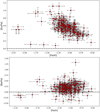 |
Fig. 2 Abundance ratios for the analysed SMC stars: [Eu/Fe] (top panel) and [Ba/Fe] (bottom panel) as a function of [Fe/H]. The dashed horizontal lines mark the solar value. |
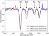 |
Fig. 3 Comparison between VLT-FLAMES spectra of three stars with similar metallicities and stellar parameters but different [Eu/Fe] abundances: 4685582751830393088 (Teff = 3881 K and log g = 0.50, green), 4687249169089083136 (Teff = 4054 K and log g = 0.45, red), and 4684827460356570624 (Teff = 4087 K and log g = 0.61, blue). The arrows mark the position of the Eu II line at 6645 Å analysed in this work and of the adjacent absorption features. |
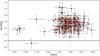 |
Fig. 4 [Eu/Mg] as a function of [Fe/H] for the spectroscopic sample discussed in this study. |
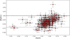 |
Fig. 5 [Ba/Eu] as a function of [Fe/H] for the spectroscopic sample discussed in this study. The black dotted line in the bottom panel marks [Ba/Eu]=−0.69 dex, which is indicative of pure r-process content in the stars (Arlandini et al. 1999). |
5 Discussion
The observed [Eu/Fe] versus [Fe/H] abundance pattern in the SMC as shown in the top panel of Fig. 2 can be viewed in light of the standard framework used to interpret the Eu abundance trends in the MW. At low metallicities, the small number of targets prevents us from drawing definitive conclusions, but the large star-to-star scatter seems to suggest an inhomogeneous mixing in the gas of the SMC in its early epochs. A similar [Eu/Fe] scatter is also observed among the MW Halo stars (see e.g. McWilliam et al. 1995; Ryan et al. 1996; Burris et al. 2000; François et al. 2007, 2024). As discussed in Paper I, the SMC stars with [Fe/H]<-1.3 dex were likely formed in the first 1-2 Gyr of life of the galaxy (see, e.g. the theoretical age-metallicity relation by Pagel & Tautvaisiene 1998). As the production of Eu is dominated by rare sources, with both prompt and delayed sources of enrichment constituting a minority in massive stars (m ≳ 8M⊙, which are already small in number due to the power-law nature of the initial stellar mass function), the observed star-to-star scatter reflects the stochastic nature of these sites of production (e.g. Cescutti et al. 2015; Cavallo et al. 2021; Hirai et al. 2022). At higher metallicities, a clear decreasing trend in [Eu/Fe] with [Fe/H] is instead found. This can be attributed to the onset of the Type Ia SNe that produce Fe but not Eu, thus reducing [Eu/Fe]. Indeed, this progressive decrease in [Eu/Fe] is in theoretical agreement with the flat trend in [Eu/Mg] (Fig. 4), as Mg is not produced by Type Ia SNe but only in massive stars (see e.g. Palla 2021). On the other hand, the decline of [Eu/Mg] as a function of [Mg/H] suggests that increasing the bulk of the metals (traced by oxygen, which has a timescale of enrichment similar to Mg) causes the relative contribution of r- and α-processes to decrease, therefore indicating the reduction of the Eu production in massive stellar populations. Nonetheless, as already stated in Section 4, some caution is needed in evaluating this trend due to the prominent uncertainties for the Mg abundances. At the same time, the [Ba/Eu] trend increases with metallicity, passing from low values, compatible with the theoretical expectations for pure r-process production (Arlandini et al. 1999; Sneden et al. 2008), to supersolar values. The increase of [Ba/Eu] with metallicity, starting at [Fe/H] ~ −1 dex in the solar vicinity and at lower [Fe/H] values in the Magellanic Clouds, is readily explained as being due to the delayed release of s-process elements in the interstellar medium by AGB stars (e.g. Karakas 2010; Cristallo et al. 2015), which occurs at lower metallicities in smaller galaxies (see below). Indeed, as [Fe/H] increases, the contribution from low- and intermediate-mass AGB stars eventually becomes the main production channel for Ba.
To better understand the chemical abundance trends displayed in Fig. 2, 4, and 5, it is crucial to compare the abundance patterns of [Eu/Fe], [Eu/Mg], and [Ba/Eu] as a function of [Fe/H] as measured in the SMC stars with the patterns observed in other systems. In this context, the MW and the LMC are the two most natural candidates to look at. The MW serves as the standard benchmark for chemical abundance trends within the Local Group, while the LMC, as a companion galaxy to the SMC, occupies an intermediate scale in galactic mass between the SMC and the MW (Stanimirovic et al. 2004; Erkal et al. 2019; Callingham et al. 2019).
In Fig. 7 we show the abundance trends in our SMC stars as compared with the observations in the MW and in the LMC. To compare our observed trends with those of the MW and the LMC, we considered the compilation of abundances for MW stars available in the SAGA database (Suda et al. 2008) and the sample of LMC giant stars analysed by Van der Swaelmen et al. (2013). The mean trends of the three galaxies (solid lines in Fig. 7) are represented using a non-parametric Gaussian KDE (Kernel Density Estimation) regression together with their corresponding 1σ confidence intervals (shaded areas). Regarding [Eu/Fe] (Fig. 7, top panel), the SMC and LMC exhibit similar trends, with comparable median [Eu/Fe] in the metallicity range in common between the two galaxies (−1.2≲[Fe/H]/dex≲-0.6 ), suggesting similar timescales for the r-process in the two Clouds. Both galaxies, however, show [Eu/Fe] values on average higher than 0.2 dex with respect to MW stars at a similar [Fe/H]. The most pronounced difference between the trends observed in the Magellanic Clouds and that of the Galaxy is seen for [Eu/Mg], displayed in the central panel of Fig. 7. Indeed, the SMC and LMC show comparable values in abundance ratios as happens for [Eu/Fe], but here their values of [Eu/Mg] reveal a much more significant offset (by ∼0.5 dex) than the trend observed for MW stars. Similar to [Eu/Fe], the comparable trends of [Eu/Mg] in the SMC and the LMC point out similar timescales also for α-processes in the two Clouds.
For the [Ba/Eu] abundance pattern (Fig. 7, bottom panel), we also observed that the abundance ratio is generally enhanced in the Magellanic Clouds relative to the MW at metallicities of [Fe/H]≳ –1 dex, with the [Ba/Eu] in the high-metallicity end of the LMC distribution being larger by ∼0.3 dex than that observed in the MW. However, in this panel we note that rather than an offset at all the overlapping metallicities (as in the case of [Eu/Mg]), the difference in the [Ba/Eu] abundance is the result of a progressive detachment of the SMC and LMC abundance trends from that of the MW with increasing metallicity.
Figure 7 clearly highlights an excess in r-process (and therefore of Eu) production in the SMC relative to the Galaxy. Indeed, the panels showing [Eu/Fe] and [Eu/Mg] display values in the SMC comparable with those in the LMC, but the values are enhanced with respect to what is observed in the MW, especially for [Eu/Mg]. This result is consistent with what has been observed in other Local Group galaxies with a star formation efficiency less pronounced than that of the MW, for instance, the remnant of the Sagittarius dSph (Liberatori et al. 2025), Fornax (Letarte et al. 2010), and Sculptor dSphs (Hill et al. 2019). All of these galaxies appear to share high [Eu/Fe] and simultaneously low [a/Fe] values, resulting in [Eu/a] abundance ratios being markedly different between the MW and smaller galaxies (see also Palla et al. 2025).
Moreover, this finding is also consistent with the evidence that stars and globular clusters in the MW dynamically associated with merger events involving primitive satellite galaxies are characterised, at least for [Fe/H]>-1.5 dex, by higher [Eu/a] abundance ratios compared to in situ stars (Monty et al. 2024; Ernandes et al. 2024; Ceccarelli et al. 2024). Therefore, the findings in this work point towards a ubiquitous r-process enhancement across MW satellite galaxies, from the most massive systems (LMC and SMC) to the least massive dSphs (Sculptor), urging further theoretical work to explain (with a self-consistent theory) the r-process abundance patterns observed throughout the Local Group. In this regard, Palla et al. (2025) have suggested an increased production in the r-process from delayed sources (e.g. NSMs) for Z≲ 0.1 Z⊙ to match the enhanced [Eu/Fe] and [Eu/α] observed in several Local Group dSphs (Sagittarius, Fornax, Sculptor) with the observed trends in the MW. A similar scenario, but based on an increased production in the r-process from prompted sources, has been proposed by Tsujimoto (2024) to explain the observed Eu abundances in the LMC. It is worth noting that the observed pattern in the [Eu/Mg] versus [Mg/H] diagram is in line with this claim, as Mg traces the enrichment timescale of the bulk of metals, and a progressive decrease in the r-process to α-element ratio should mirror a fading contribution by an r-process source.
However, further investigations are definitely needed in this context, also considering that theoretical predictions have to match observations not only for Eu and metals up to the iron-peak (e.g. Fe, Mg) but also for other neutron-capture elements, which receive a non-negligible contribution from the r-process to their production. In this regard, the bottom panel of Fig. 7 is highly instructive, showing the differences in the trends of [Ba/Eu] in the SMC, LMC, and the Galaxy at different metallic-ities. At variance with what happens for [Eu/Mg], here we note a rather ‘standard, behaviour for the [Ba/Eu] abundance ratio, with an enhancement in Ba at lower metallicities for systems with a lower stellar mass and star formation efficiency. Indeed, the contribution expected from the first low-mass AGB stars (producing s-process) is expected to take place at lower metallicities in the latter systems (Venn et al. 2004; Tolstoy et al. 2009) where the chemical enrichment proceeds at a slower pace (Matteucci 2012).
The stronger production of r-process elements up to [Fe/H]–1 dex proposed by Palla et al. (2025), however, goes in the opposite direction, as it suggests a decrease in the relative s-process contribution to Ba production, therefore leading to a flatter trend. A possible solution can be seen in the context of a different initial stellar mass function in dwarf galaxies, with the initial stellar mass function of the Magellanic Clouds being more bottom-heavy and top-light, therefore balancing the overproduction of Eu with more Ba production by low-mass AGB stars. This solution agrees well with the multiple indications (e.g. Lee et al. 2009; Pflamm-Altenburg & Kroupa 2009; Jeřábková et al. 2018; Watts et al. 2018) pointing towards a reduction in the relative fraction of massive stars in the stellar populations of dwarf galaxies. However, a thorough discussion on this matter is beyond the scope of this paper, so it will be addressed in a future paper of this series (Palla et al., in prep.).
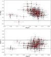 |
Fig. 6 [Eu/Mg] (top panel) and [Ba/Eu] (bottom panel) as a function of [Mg/H]. |
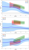 |
Fig. 7 [Eu/Fe] (top panel), [Eu/Mg] (middle panel), and [Ba/Eu] (bottom panel) vs. [Fe/H] trends for the SMC, the LMC, and the MW. The solid lines are non-parametric Gaussian KDE (Kernel Density Estimation) regressions, while the shaded areas represent the 1σ confidence interval of the regressions. The black dotted line in the bottom panel marks the value below which we have a pure r-process enrichment (Arlandini et al. 1999, see also Fig. 5). |
6 Summary and conclusions
In this study we have presented the first measurements of the [Eu/Fe] ratio in a sample of SMC stars covering a very extended (1.5 dex in [Fe/H]) metallicity range of the galaxy. The most interesting feature we find from this dataset is the enhanced [Eu/Mg] in the SMC, whose values are comparable with those measured in the LMC and in other dSphs but significantly higher than the MW values. Our result confirms that the Local Group galaxies characterised by a star formation efficiency lower than than that of the MW (i.e. Sagittarius, isolated dSphs, Magellanic Clouds) exhibit clearly distinct [Eu/Fe] and [Eu/Mg] with respect to the MW stars, therefore supporting the idea that [Eu/α] can be used as a powerful diagnostic to distinguish accreted stars from those formed in situ (Monty et al. 2024; Ernandes et al. 2024; Ceccarelli et al. 2024), at least at intermediate and high metallicity. On the other hand, the SMC exhibits a standard behaviour for [Ba/Eu] that increases by increasing [Fe/H], indicating a progressive increase of the contribution of low-and intermediate-mass AGB stars with age. The investigation of neutron-capture elements in external galaxies, such as the Magellanic Clouds, is therefore a field of research fundamental for Galactic archaeology and for our understanding of the MW assembly history.
Data availability
Tables 1 and 2 are available at the CDS via https://cdsarc.cds.unistra.fr/viz-bin/cat/J/A+A/705/A31.
Acknowledgements
We thank the referee, Sten Hasselquist, for the useful comments and suggestions. A.M., M.P. and D.R. acknowledge support from the project “LEGO - Reconstructing the building blocks of the Galaxy by chemical tagging” (PI: A. Mucciarelli) granted by the Italian MUR through contract PRIN 2022LLP8TK_001.
References
- Abbott, B. P., Abbott, R., Abbott, T. D., et al. 2017, Phys. Rev. Lett., 119, 161101 [Google Scholar]
- Andrae, R., Fouesneau, M., Creevey, O., et al. 2018, A&A, 616, A8 [NASA ADS] [CrossRef] [EDP Sciences] [Google Scholar]
- Arcones, A., & Thielemann, F.-K. 2023, A&A Rev., 31, 1 [NASA ADS] [CrossRef] [Google Scholar]
- Argast, D., Samland, M., Thielemann, F. K., & Qian, Y. Z. 2004, A&A, 416, 997 [NASA ADS] [CrossRef] [EDP Sciences] [Google Scholar]
- Arlandini, C., Kappeler, F., Wisshak, K., et al. 1999, ApJ, 525, 886 [NASA ADS] [CrossRef] [Google Scholar]
- Burbidge, E. M., Burbidge, G. R., Fowler, W. A., & Hoyle, F. 1957, Rev. Mod. Phys., 29, 547 [NASA ADS] [CrossRef] [Google Scholar]
- Burris, D. L., Pilachowski, C. A., Armandroff, T. E., et al. 2000, ApJ, 544, 302 [Google Scholar]
- Callingham, T. M., Cautun, M., Deason, A. J., et al. 2019, MNRAS, 484, 5453 [Google Scholar]
- Carney, B. W., Latham, D. W., Stefanik, R. P., Laird, J. B., & Morse, J. A. 2003, AJ, 125, 293 [NASA ADS] [CrossRef] [Google Scholar]
- Cavallo, L., Cescutti, G., & Matteucci, F. 2021, MNRAS, 503, 1 [CrossRef] [Google Scholar]
- Cayrel, R., Depagne, E., Spite, M., et al. 2004, A&A, 416, 1117 [NASA ADS] [CrossRef] [EDP Sciences] [Google Scholar]
- Ceccarelli, E., Mucciarelli, A., Massari, D., Bellazzini, M., & Matsuno, T. 2024, A&A, 691, A226 [NASA ADS] [CrossRef] [EDP Sciences] [Google Scholar]
- Cescutti, G., Romano, D., Matteucci, F., Chiappini, C., & Hirschi, R. 2015, A&A, 577, A139 [NASA ADS] [CrossRef] [EDP Sciences] [Google Scholar]
- Côté, B., Eichler, M., Arcones, A., et al. 2019, ApJ, 875, 106 [Google Scholar]
- Cristallo, S., Straniero, O., Piersanti, L., & Gobrecht, D. 2015, ApJS, 219, 40 [Google Scholar]
- De Leo, M., Carrera, R., Noël, N. E. D., et al. 2020, MNRAS, 495, 98 [Google Scholar]
- Erkal, D., Belokurov, V., Laporte, C. F. P., et al. 2019, MNRAS, 487, 2685 [Google Scholar]
- Ernandes, H., Feuillet, D., Feltzing, S., & Skúladóttir, Á. 2024, A&A, 691, A333 [NASA ADS] [CrossRef] [EDP Sciences] [Google Scholar]
- François, P., Depagne, E., Hill, V., et al. 2007, A&A, 476, 935 [Google Scholar]
- François, P., Cescutti, G., Bonifacio, P., et al. 2024, A&A, 686, A295 [NASA ADS] [CrossRef] [EDP Sciences] [Google Scholar]
- Gaia Collaboration (Babusiaux, C., et al.) 2018, A&A, 616, A10 [NASA ADS] [CrossRef] [EDP Sciences] [Google Scholar]
- Gaia Collaboration (Brown, A. G. A., et al.) 2021, A&A, 649, A1 [NASA ADS] [CrossRef] [EDP Sciences] [Google Scholar]
- Graczyk, D., Pietrzynski, G., Thompson, I. B., et al. 2014, ApJ, 780, 59 [Google Scholar]
- Hekker, S., Snellen, I. A. G., Aerts, C., et al. 2008, A&A, 480, 215 [NASA ADS] [CrossRef] [EDP Sciences] [Google Scholar]
- Helmi, A., Babusiaux, C., Koppelman, H. H., et al. 2018, Nature, 563, 85 [Google Scholar]
- Hill, V., Skúladóttir, Á., Tolstoy, E., et al. 2019, A&A, 626, A15 [NASA ADS] [CrossRef] [EDP Sciences] [Google Scholar]
- Hirai, Y., Beers, T. C., Chiba, M., et al. 2022, MNRAS, 517, 4856 [NASA ADS] [CrossRef] [Google Scholar]
- Jerábková, T., Hasani Zonoozi, A., Kroupa, P., et al. 2018, A&A, 620, A39 [NASA ADS] [CrossRef] [EDP Sciences] [Google Scholar]
- Karakas, A. I. 2010, MNRAS, 403, 1413 [NASA ADS] [CrossRef] [Google Scholar]
- Kobayashi, C., Karakas, A. I., & Lugaro, M. 2020, ApJ, 900, 179 [Google Scholar]
- Kramida, A., Yu. Ralchenko, Reader, J., & NIST ASD Team 2024, NIST Atomic Spectra Database (ver. 5.12), [Online]. Available: https://physics.nist.gov/asd [2025, July 9]. National Institute of Standards and Technology, Gaithersburg, MD. [Google Scholar]
- Kurucz, R. L. 2005, Mem. Soc. Astron. It. Suppl., 8, 14 [Google Scholar]
- Lawler, J. E., Wickliffe, M. E., den Hartog, E. A., & Sneden, C. 2001, ApJ, 563, 1075 [CrossRef] [Google Scholar]
- Lee, J. C., Gil de Paz, A., Tremonti, C., et al. 2009, ApJ, 706, 599 [NASA ADS] [CrossRef] [Google Scholar]
- Letarte, B., Hill, V., Tolstoy, E., et al. 2010, A&A, 523, A17 [NASA ADS] [CrossRef] [EDP Sciences] [Google Scholar]
- Liberatori, A., Alvarez Garay, D. A., Palla, M., et al. 2025, A&A, 699, A356 [NASA ADS] [CrossRef] [EDP Sciences] [Google Scholar]
- Lindegren, L., Hernández, J., Bombrun, A., et al. 2018, A&A, 616, A2 [NASA ADS] [CrossRef] [EDP Sciences] [Google Scholar]
- Matsuno, T., Dodd, E., Koppelman, H. H., et al. 2022, A&A, 665, A46 [NASA ADS] [CrossRef] [EDP Sciences] [Google Scholar]
- Matteucci, F. 2012, Chemical Evolution of Galaxies (Berlin: Springer) [Google Scholar]
- Matteucci, F. 2021, A&A Rev., 29, 5 [NASA ADS] [CrossRef] [Google Scholar]
- McCall, M. L. 2004, AJ, 128, 2144 [Google Scholar]
- McWilliam, A., Preston, G. W., Sneden, C., & Searle, L. 1995, AJ, 109, 2757 [Google Scholar]
- Molero, M., Romano, D., Reichert, M., et al. 2021, MNRAS, 505, 2913 [NASA ADS] [CrossRef] [Google Scholar]
- Molero, M., Magrini, L., Matteucci, F., et al. 2023, MNRAS, 523, 2974 [NASA ADS] [CrossRef] [Google Scholar]
- Monty, S., Belokurov, V., Sanders, J. L., et al. 2024, MNRAS, 533, 2420 [NASA ADS] [CrossRef] [Google Scholar]
- Mucciarelli, A. 2011, A&A, 528, A44 [NASA ADS] [CrossRef] [EDP Sciences] [Google Scholar]
- Mucciarelli, A., & Bonifacio, P. 2020, A&A, 640, A87 [NASA ADS] [CrossRef] [EDP Sciences] [Google Scholar]
- Mucciarelli, A., Origlia, L., & Ferraro, F. R. 2010, ApJ, 717, 277 [NASA ADS] [CrossRef] [Google Scholar]
- Mucciarelli, A., Bellazzini, M., & Massari, D. 2021, A&A, 653, A90 [NASA ADS] [CrossRef] [EDP Sciences] [Google Scholar]
- Mucciarelli, A., Minelli, A., Bellazzini, M., et al. 2023a, A&A, 671, A124 [NASA ADS] [CrossRef] [EDP Sciences] [Google Scholar]
- Mucciarelli, A., Minelli, A., Lardo, C., et al. 2023b, A&A, 677, A61 [NASA ADS] [CrossRef] [EDP Sciences] [Google Scholar]
- Mucciarelli, A., Bonifacio, P., & Lardo, C. 2025, arXiv e-prints [arXiv:2511.10737] [Google Scholar]
- Nidever, D. L., Hasselquist, S., Hayes, C. R., et al. 2020, ApJ, 895, 88 [Google Scholar]
- Nissen, P. E., & Schuster, W. J. 2010, A&A, 511, L10 [NASA ADS] [CrossRef] [EDP Sciences] [Google Scholar]
- Pagel, B. E. J., & Tautvaisiene, G. 1998, MNRAS, 299, 535 [Google Scholar]
- Palla, M. 2021, MNRAS, 503, 3216 [Google Scholar]
- Palla, M., Molero, M., Romano, D., & Mucciarelli, A. 2025, A&A, 699, A209 [NASA ADS] [CrossRef] [EDP Sciences] [Google Scholar]
- Pasquini, L., Avila, G., Blecha, A., et al. 2002, The Messenger, 110, 1 [Google Scholar]
- Patel, A., Metzger, B. D., Cehula, J., et al. 2025, ApJ, 984, L29 [Google Scholar]
- Pflamm-Altenburg, J., & Kroupa, P. 2009, MNRAS, 397, 488 [CrossRef] [Google Scholar]
- Pian, E., D’Avanzo, P., Benetti, S., et al. 2017, Nature, 551, 67 [Google Scholar]
- Prantzos, N., Abia, C., Cristallo, S., Limongi, M., & Chieffi, A. 2020, MNRAS, 491, 1832 [Google Scholar]
- Reggiani, H., Schlaufman, K. C., Casey, A. R., Simon, J. D., & Ji, A. P. 2021, AJ, 162, 229 [NASA ADS] [CrossRef] [Google Scholar]
- Reichert, M., Hansen, C. J., Hanke, M., et al. 2020, A&A, 641, A127 [NASA ADS] [CrossRef] [EDP Sciences] [Google Scholar]
- Ryan, S. G., Norris, J. E., & Beers, T. C. 1996, ApJ, 471, 254 [Google Scholar]
- Sbordone, L., Bonifacio, P., Buonanno, R., et al. 2007, A&A, 465, 815 [NASA ADS] [CrossRef] [EDP Sciences] [Google Scholar]
- Schlafly, E. F., & Finkbeiner, D. P. 2011, ApJ, 737, 103 [Google Scholar]
- Shigeyama, T., & Tsujimoto, T. 1998, ApJ, 507, L135 [NASA ADS] [CrossRef] [Google Scholar]
- Siegel, D. M., Barnes, J., & Metzger, B. D. 2019, Nature, 569, 241 [Google Scholar]
- Skrutskie, M. F., Cutri, R. M., Stiening, R., et al. 2006, AJ, 131, 1163 [NASA ADS] [CrossRef] [Google Scholar]
- Sneden, C., Cowan, J. J., & Gallino, R. 2008, ARA&A, 46, 241 [Google Scholar]
- Stanimirovic, S., Staveley-Smith, L., & Jones, P. A. 2004, ApJ, 604, 176 [Google Scholar]
- Subramanian, S., & Subramaniam, A. 2009, A&A, 496, 399 [NASA ADS] [CrossRef] [EDP Sciences] [Google Scholar]
- Suda, T., Katsuta, Y., Yamada, S., et al. 2008, PASJ, 60, 1159 [NASA ADS] [Google Scholar]
- Thielemann, F. K., Eichler, M., Panov, I. V., & Wehmeyer, B. 2017, Ann. Rev. Nucl. Part. Sci., 67, 253 [Google Scholar]
- Tolstoy, E., Hill, V., & Tosi, M. 2009, ARA&A, 47, 371 [Google Scholar]
- Tonry, J., & Davis, M. 1979, AJ, 84, 1511 [Google Scholar]
- Tsujimoto, T. 2024, ApJ, 967, 85 [Google Scholar]
- Van der Swaelmen, M., Hill, V., Primas, F., & Cole, A. A. 2013, A&A, 560, A44 [NASA ADS] [CrossRef] [EDP Sciences] [Google Scholar]
- Venn, K. A., Irwin, M., Shetrone, M. D., et al. 2004, AJ, 128, 1177 [NASA ADS] [CrossRef] [Google Scholar]
- Watson, D., Hansen, C. J., Selsing, J., et al. 2019, Nature, 574, 497 [NASA ADS] [CrossRef] [Google Scholar]
- Watts, A. B., Meurer, G. R., Lagos, C. D. P., et al. 2018, MNRAS, 477, 5554 [NASA ADS] [CrossRef] [Google Scholar]
- Winteler, C., Käppeli, R., Perego, A., et al. 2012, ApJ, 750, L22 [Google Scholar]
All Tables
All Figures
|
Fig. 1 Difference between the RVs derived in this study and those in Paper I as a function of the Gaia DR3 G magnitude. The red circles are stars with discrepant RV differences after a 3σ-clipping iterative procedure. |
| In the text | |
|
Fig. 2 Abundance ratios for the analysed SMC stars: [Eu/Fe] (top panel) and [Ba/Fe] (bottom panel) as a function of [Fe/H]. The dashed horizontal lines mark the solar value. |
| In the text | |
|
Fig. 3 Comparison between VLT-FLAMES spectra of three stars with similar metallicities and stellar parameters but different [Eu/Fe] abundances: 4685582751830393088 (Teff = 3881 K and log g = 0.50, green), 4687249169089083136 (Teff = 4054 K and log g = 0.45, red), and 4684827460356570624 (Teff = 4087 K and log g = 0.61, blue). The arrows mark the position of the Eu II line at 6645 Å analysed in this work and of the adjacent absorption features. |
| In the text | |
|
Fig. 4 [Eu/Mg] as a function of [Fe/H] for the spectroscopic sample discussed in this study. |
| In the text | |
|
Fig. 5 [Ba/Eu] as a function of [Fe/H] for the spectroscopic sample discussed in this study. The black dotted line in the bottom panel marks [Ba/Eu]=−0.69 dex, which is indicative of pure r-process content in the stars (Arlandini et al. 1999). |
| In the text | |
|
Fig. 6 [Eu/Mg] (top panel) and [Ba/Eu] (bottom panel) as a function of [Mg/H]. |
| In the text | |
|
Fig. 7 [Eu/Fe] (top panel), [Eu/Mg] (middle panel), and [Ba/Eu] (bottom panel) vs. [Fe/H] trends for the SMC, the LMC, and the MW. The solid lines are non-parametric Gaussian KDE (Kernel Density Estimation) regressions, while the shaded areas represent the 1σ confidence interval of the regressions. The black dotted line in the bottom panel marks the value below which we have a pure r-process enrichment (Arlandini et al. 1999, see also Fig. 5). |
| In the text | |
Current usage metrics show cumulative count of Article Views (full-text article views including HTML views, PDF and ePub downloads, according to the available data) and Abstracts Views on Vision4Press platform.
Data correspond to usage on the plateform after 2015. The current usage metrics is available 48-96 hours after online publication and is updated daily on week days.
Initial download of the metrics may take a while.