| Issue |
A&A
Volume 705, January 2026
|
|
|---|---|---|
| Article Number | A116 | |
| Number of page(s) | 6 | |
| Section | The Sun and the Heliosphere | |
| DOI | https://doi.org/10.1051/0004-6361/202557267 | |
| Published online | 13 January 2026 | |
Center-to-limb variations of the He I 10 830 Å triplet
1
Leibniz-Institut für Astrophysik Potsdam (AIP) An der Sternwarte 16 14482 Potsdam, Germany
2
Instituto de Astrofísica de Canarias (IAC) Vía Láctea s/n E-38205 La Laguna Tenerife, Spain
3
Universidad de La Laguna, Departamento de Astrofísica E-38206 La Laguna Tenerife, Spain
★ Corresponding author: This email address is being protected from spambots. You need JavaScript enabled to view it.
Received:
16
September
2025
Accepted:
18
November
2025
Abstract
We present high-resolution spectroscopic observations of the quiet-Sun center-to-limb variations (CLV) of the He I triplet at 10 830 Å and the nearby Si I 10 827 Å line, observed with GREGOR Infrared Spectrograph (GRIS) and the improved High-resolution Fast Imager (HiFI+). The observations cover the interval μ = [0.1, 1.0], where μ is the cosine of the heliocentric angle. At each μ position, the spectra were spatially averaged over 0.02 μ and the resulting CLVs were given both as these averaged data points and as smooth polynomial curves fitted across each wavelength point. The He I spectra were inverted using the HAnle and ZEeman Light (HAZEL) code, showing an increase in optical depth towards the limb and a reversed convective blueshift for the red component, while the blue component was entirely absent. In addition, we found a strong increase in the steepness of the He I CLV compared to that of the nearby continuum. The Si I showed a behavior more typical of photospheric lines, namely shallower CLV, a reduction in width and depth, and a more typical convective blueshift.
Key words: atomic data / radiative transfer / techniques: spectroscopic / Sun: abundances / Sun: chromosphere
© The Authors 2026
 Open Access article, published by EDP Sciences, under the terms of the Creative Commons Attribution License (https://creativecommons.org/licenses/by/4.0), which permits unrestricted use, distribution, and reproduction in any medium, provided the original work is properly cited.
This article is published in open access under the Subscribe to Open model. This email address is being protected from spambots. You need JavaScript enabled to view it. to support open access publication.
1. Introduction
The He I triplet at 10 830 Å is a set of optically thin chromospheric lines that are sensitive to the overlying corona. They arise from a transition from the long-lived (metastable) 23S state, which is part of the triplet (S = 1) system of neutral helium. This is because the transition to the energetically lower singlet state is forbidden, effectively trapping the population in the triplet level (Lagg 2007; Leenaarts et al. 2016; Libbrecht et al. 2021). There are currently three processes that are known to populate these levels: (1) thermal collisional excitation; (2) photoionization-recombination from He II under UV illumination; and (3) nonthermal excitation from electron beams (e.g., Goldberg 1939; Kerr et al. 2021; Leenaarts et al. 2025).
Two of the triplet lines are heavily blended, with their cores forming roughly 0.1 Å apart, which we refer to as the red component. The remaining line, called the blue component, forms further away at 10 829 Å, but has a much smaller line depth (e.g., Kaifler et al. 2022).
The He I triplet is uniquely sensitive to both the Zeeman and Hanle effects, making it a strong diagnostic for both strong and weak magnetic fields (Trujillo Bueno et al. 2002; Kuckein et al. 2009; Bethge et al. 2011). Combined with its strong coupling to the overlying corona, this makes the triplet a valuable probe of coronal influences on the chromosphere, including the effects of coronal holes and flares (Malanushenko & Baranovsky 2001; Xu et al. 2022; Anan et al. 2018; Kuckein et al. 2025). Unlike most chromospheric lines, the triplet generally appears in absorption in active regions, producing dark plages and flares that remain in absorption for the majority of their lifetime, although transient brightenings are occasionally observed (e.g., Libbrecht 2019; De Wilde et al. 2025; Marena et al. 2025.
The He I 10 830 Å line is also a popular tool for detecting evaporation in exoplanet atmospheres, as its abundance makes it relatively easy to observe compared to other elements. Moreover, in contrast to Lyα, it does not suffer from extinction by the interstellar medium or contamination from geocoronal emission (Seager & Sasselov 2000; Oklopčić & Hirata 2018; Spake et al. 2018; Cauley et al. 2018). However, the aforementioned sensitivity to stellar activity does strongly influence the signal of the He I 10 830 Å line in exoplanet atmospheres (Poppenhaeger 2022; Sanz-Forcada et al. 2025), meaning that rapidly evolving features could bias exoplanet transit observations.
In this work, we provide a detailed set of the quiet-Sun CLV of the He I triplet and its surroundings. This will enable subsequent modeling studies to benchmark the accuracy of their models against our CLV, as is typically done for other lines (e.g., Unsöld 1955; Vernazza et al. 1976; Bjørgen et al. 2018; Alsina Ballester et al. 2021). Other studies use such profiles as initial boundary conditions to construct radiative transfer models of chromospheric and coronal structures (e.g., Gunár et al. 2020, 2021; Rachmeler et al. 2022) and to infer the formation height of the lines (Wittmann 1976). The CLV of spectral lines is also a popular tool for abundance studies (e.g., Pereira et al. 2009; Bergemann et al. 2021; Pietrow et al. 2023a) and a crucial input for pseudo-Sun-as-a-star studies (Pietrow & Pastor Yabar 2024; De Wilde et al. 2025), where quiet disks are built around observations with a limited field-of-view (FOV).
2. Observations and data processing
The observations were acquired with the 1.5-meter GREGOR solar telescope (Schmidt et al. 2012; Kleint et al. 2020) using the improved High-resolution Fast Imager (HIFI+; Denker et al. 2023) and the GREGOR Infrared Spectrograph (GRIS; Collados et al. 2012; Regalado Olivares et al. 2024). The data consist of a sparse mosaic spanning one solar radius, taken between 08:03 UT and 09:09 UT on 27 May 2024 (see Fig. 1 and Table 1). Each pointing consisted of 40 steps with a 0.5″ step size of the 60″ slit, which is sampled at 0.135″ intervals.
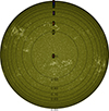 |
Fig. 1. Solar disk with the seven pointings used in this work. Ten concentric rings from μ = 0.9 to μ = 0.0 indicate steps in heliocentric angle. The background shows an AIA 1600 Å image (Lemen et al. 2012) taken at 08:10:38 UT on the same day as the observations. |
GRIS raster pointings.
For the GRIS data, a careful wavelength calibration was performed to accurately track the Doppler shifts of the faint triplet in the quiet Sun. The spectral sampling of 14.678 mÅ pixel−1 was obtained from the data reduction pipeline of GRIS (Collados 1999, 2003), which uses an average quiet-Sun profile at disk center obtained from the flat field data and matches it to the Livingston & Wallace (1991) Fourier Transform Spectrometers (FTS) atlas. The telluric line at 10 832.108 Å was then used to determine the zero point of the wavelength scale. Finally, the wavelength array was corrected for the gravitational redshift, the rotation of the Earth and the Sun, and the orbital motion of the Earth around the Sun. More details about these wavelength calibration steps are given in the appendices of Martínez Pillet et al. (1997) and Kuckein et al. (2012). This calibration resulted in a spectral window covering the wavelength range from 10 818.50 Å to 10 833.31 Å at a spectral resolution of R ∼ 190 000 (see Figs. 2, 3, and 4).
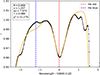 |
Fig. 2. HAZEL fit (orange) of He I triplet observations at μ = 1 (black dashed). The rest velocities of the red and blue components are marked with vertical lines in the respective colors. Basic information and the best-fit parameters are given in the box at the upper-left corner. These include the heliocentric angle, θ, the Doppler velocity, v, the Doppler width, Δv, the optical depth, τ, and the quality of fit, χ2. |
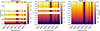 |
Fig. 3. CLV maps of the GRIS spectral window. Mean CLV profiles (left) across the full μ-range. Oscillations are visible across the entire range. Cleaned profiles (middle) after polynomial fitting. Normalized profiles (right) of the middle panel, showing the relative CLV behavior across the spectral window. |
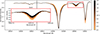 |
Fig. 4. One-dimensional version of the data in Fig. 3 (right panel), showing the changes in the spectrum as a function of μ. A zoomed-in window focuses on the He I line at 10 830 Å. The black vertical line marks the wavelength of the intensity calibration. |
The spectral line-spread function (LSF) characterizes the instrumental spectral resolution of GRIS, while the spectral stray light (or veil) represents a wavelength-independent constant contribution added to the measured intensity. Both quantities were determined by comparing an average quiet-Sun spectrum from the GRIS data with the FTS atlas, following Sect. 3 of Borrero et al. (2016). The FTS spectrum was convolved with a Gaussian profile and combined with a constant veil term in the form of
 (1)
(1)
Here,  is the GRIS-simulated average quiet-Sun intensity profile, Ifts the atlas profile, g a Gaussian function with width σ, ν is the fraction of spectral scattered light, and Ic, fts is the continuum intensity of the atlas close to the line.
The best agreement was obtained by minimizing the χ2 between the observed and synthetic spectra ( ). The resulting parameters are a Gaussian width of σ = 3.77 pixels (or 55.34 mÅ), which corresponds to a FWHM of 130.04 mÅ, and a spectral stray light fraction of 3.8%.
For the HiFI+ data, only the G-band channel was used since it was the longest wavelength channel available with photospheric information close to that of the Helioseismic and Magnetic Imager (HMI; Scherrer et al. 2012) on board the Solar Dynamics Observatory (SDO; Pesnell et al. 2012). These data were processed with the sTools software (Kuckein et al. 2017), using the Kiepenheuer Institute Speckle Imaging Package (KISIP; Wöger et al. 2008). The speckle-restored time series covers a FOV of 71″ × 60″ with a plate scale of 0.028″ pixel−1.
3. Methods
In this section, we discuss the data processing steps to create the CLV curves. We also present the steps we used to invert the curves.
3.1. CLV curve generation
Due to its high spatial resolution, the HiFI+ data were used as context information and the first frame of each observation was used to align the GREGOR FOV with respect to the HMI data. Typically, such alignments are made with a cross-correlation algorithm (e.g., Cauzzi & Reardon 2012; Hammerschlag et al. 2013). However, they have been shown not to work on quiet-Sun regions close to the limb (Pastor Yabar et al. 2020; Pietrow et al. 2023b). Instead, a manual approach is used instead, for instance, with the mosaic alignment tools from the ISPy library (Díaz Baso et al. 2021), where bright points are used for reference. Based on the jitter of the limb, we estimated our alignment accuracy to be about two GRIS pixels, or 0.27″, which is negligible everywhere except at the extreme limb.
Once aligned to HMI, the target frames of both HiFI+ and GRIS were aligned to obtain an accurate pointing for the GRIS frames. Afterwards, a μ-value was assigned to each spectrum, and the array was sorted. In Pietrow et al. (2023b), the intensity calibration was carried out by fitting a polynomial between three disk center observations, which were taken at the start, middle, and end of the mosaic to compensate for atmospheric extinction changes throughout the observing period. However, this approach could not be used, as only two disk center measurements were taken at either ends of the observations. Therefore, a new approach was taken where a continuum point, in this case 10 823 Å, was chosen and each μ-position was set to match the predicted intensity of Neckel & Labs (1994) at that wavelength as the rest of the spectrum is scaled accordingly. This approach is not valid beyond μ = 0.08, as these values must be extrapolated from the rest of the fit (Fig. 6 in Pietrow et al. 2023b). For this reason, we did not fit our CLV beyond μ = 0.1.
We average the spectra over windows of 0.02 μ for each of 10 mu positions, ranging from 1.0 to 0.1 in steps of 0.1. The number of pixels per bin over which we average is shown in Table 2. The first bin is limited because about half of the raster was contaminated with a small filament close to the disk center. The resulting CLV is shown as a function of radius in the first panel of Fig. 3 and as a function of μ in the second panel. Following the method introduced by Neckel & Labs (1994), the third panel shows the same values, but smoothed using a fourth-order polynomial fit across μ to each wavelength point. This smoothes the local intensity variations that are likely caused by small brightenings. This was especially helpful in the He I 10830 Å line core (see red line in the right panel of Fig. 5). The resulting averaged spectra exhibited small intensity oscillations over the wavelength axis. These are likely of instrumental origin and were smoothened out using a 5-pixel (90 mÅ) box filter, which lowers the spectral resolution to R ≈ 120 000. For the purposes of this work, we only considered the Stokes-I profiles, since the other Stokes profiles are too weak in the quiet Sun.
Number of points, N, per μ bin.
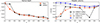 |
Fig. 5. Inferred spectral line behavior as a function of μ. Left: Optical depth τ of the He I line. Right: Doppler velocity for the median He I (black) and Si I (gray) line profiles, together with their polynomial fits shown in red and blue dashed lines, respectively. |
3.2. Inversions
We used the HAZEL code (Asensio Ramos et al. 2008) to invert the observed spectra, considering only the Stokes-I profile to retrieve a model atmosphere. The inversion strategy included a chromospheric slab model, a photospheric model, and a parametric component to account for the He I triplet, the Si I line at 10 827 Å, and the telluric line, respectively. Two inversion cycles were sufficient to achieve a good fit to the spectra (see Fig. 2).
For helium, in the first cycle, only the optical depth τ and the Doppler velocity vHe were treated as free parameters. In the second cycle, the vHe was fixed and additional parameters (e.g., the Doppler width, the β parameter, and a damping parameter) were allowed to vary. The latter two parameters primarily affect the shape of the line by modifying the depth of the core and wings. While the red component of the He I line fitted well, the blue component of the He I triplet was barely visible in our spectra and seems to mainly show up in active regions, such as the filament in the disk-center pointing (see first panel of Fig. 3). This is in line with previous observations (e.g., Avrett et al. 1994; Mauas et al. 2005; Libbrecht 2019).
For the Si I line at 10 827 Å, the HAZEL code internally employs the Stokes Inversion based on Response functions (SIR; Ruiz Cobo & del Toro Iniesta 1992) code, which assumes local thermodynamic equilibrium (LTE) and hydrostatic equilibrium. We used three nodes in the first cycle and five in the second for the temperature. All the other parameters were assumed to be constant with height, that is, they were assigned a single node in each cycle. Here, we only present the Doppler velocity vSi, as the other parameters are less reliable due to the nonLTE nature in the core of this line (e.g., Bard & Carlsson 2008).
4. Results and discussion
In this section, we discuss the results inferred from both the averaged spectra and the inversions. We first discuss the Si I and He I 10830 Å lines independently and then compare the results.
4.1. Si I line at 10 827 Å
Inspecting Fig. 4, we see that the Si I line becomes slightly shallower and loses a significant part of its width when moving toward the limb. This is a typical behavior for photospheric lines, as the inclined line of sight (LOS) decreases the contribution from the lower lying layer, which contributes most of the opacity for the line wings. It also results in a shallower temperature gradient between the center and the limb, which, in turn, results in a flatter limb-darkening curve (see Fig. 6). When the disk center is used as the velocity reference, such photospheric lines tend to show an apparent redshift (see the blue line in the right panel of Fig. 5). This phenomenon, known as convective blueshift, arises from solar granulation. At the disk center, the observed intensity is dominated by upward-moving (blueshifted) granules, whereas towards the limb, the contribution from these granules diminishes due to the viewing geometry (e.g., Löhner-Böttcher et al. 2019).
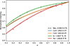 |
Fig. 6. Fitted (solid line) and mean (scattered points) CLV of the He I line core at 10 830 Å (red), the Si I line core at 10 827 Å (green), and two continuum points (blue and orange). The quiet-Sun continuum limb-darkening profile (dashed) from Neckel & Labs (1994) is overplotted for comparison. |
4.2. He I line at 10 830 Å
The He I line forms in the middle to high chromosphere (e.g., Avrett et al. 1994; Centeno et al. 2008). The off-limb emission in the line peaks at around 1.5 Mm and extends to just below 3.0 Mm, which is in line with previous measurements (e.g., de la Cruz Rodríguez et al. 2019; Libbrecht et al. 2021).
This line behaves quite differently from photospheric lines such as the aforementioned Si I line, but also from other chromospheric lines in the visible. The line profile appears both deeper and broader toward the limb (Fig. 4). The broadening is consistent with the behavior of other chromospheric lines reported by Pietrow et al. (2023b), although those lines become shallower with respect to the continuum because their CLV decreases less steeply than that of the nearby continuum. In contrast, the He I line exhibits a comparatively steeper CLV, likely because it is optically thin and, thus, it accumulates greater opacity along the slanted LOS.
The Doppler shift relation along μ is also in the opposite direction (blue) than the aforementioned photospheric Si I line (see red+black lines and blue+gray lines in the right panel of Fig. 5), resulting in a net blueshift towards the limb. The reason for this shift could be the result of an average downwards motion of the chromospheric fibrils, creating the reverse of what we see in the photosphere (Wedemeyer-Böhm et al. 2009; Ellwarth et al. 2023; Löhner-Böttcher et al. 2019), meaning that the reason for this “fibrilar redshift” is likely rooted in the downward flows in the chromospheric canopy.
The Doppler velocity at μ = 0.8 appears as an outlier relative to the overall trend (see the right panel of Fig. 5). This deviation likely reflects the strong sensitivity of the He I line to solar activity. While obvious filaments and bright points were removed prior to averaging, smaller features were retained to avoid biases from over-processing. Nevertheless, these outliers have little influence on the fitted polynomials, which yield a relatively smooth overall trend.
Finally, we note the complete absence of the line’s blue component in our observations. It is unlikely that this is an averaging effect similar to the one that causes the v and r components of the Ca II H&K lines to disappear (Druzhinin et al. 1987), since the blue component is also absent in the disk-center rasters outside the regions affected by filament contamination (see Fig. 3). The disappearance of this component is also shown in Fig. 6 of Avrett et al. (1994). However, it was not possible to reproduce it with HAZEL, indicating a possible unmodeled radiative transfer process. This question will be addressed further in a follow-up study.
4.3. Limb darkening
We present the CLV of the He I line at 10 830 Å and the Si I line at 10 827 Å, as well as that of the surrounding continuum in Fig. 6. The values of the averaged μ positions are given as scattered points and the fitted curves as solid lines. The continuum points are overplotted with the continuum CLV of Neckel & Labs (1994) to show the results of the calibration. The Si I line shows a flatter curve than the continuum profile, which is expected from higher-forming photospheric lines (e.g., Canocchi et al. 2024). The He I line displays a steeper curve than the surrounding continuum, a behavior that is inconsistent with other chromospheric lines. It is likely due to the line’s optically thin nature, which enables greater opacity buildup along inclined lines of sight. These results can be compared with synthetic spectra when the latter are convolved down to the smoothed resolution of GRIS following Eq. (1) with a σ value of 55.34 mÅ and a ν value of 3.8%.
5. Summary and conclusions
We present high-resolution CLV observations of the infrared He I line across seven disk pointings (see Fig. 1) obtained with GRIS at the 1.5-meter GREGOR solar telescope. These data were aligned to SDO/HMI using HiFI+ co-observations, after which a μ position was calculated for each pixel. The intensity was then calibrated by matching the continuum near 10 824 Å to the continuum limb-darkening atlas of Neckel & Labs (1994). The resulting CLV spectra were then averaged into ten μ positions between 0.1 and 1.0, using an averaging window of 0.02 μ (see Fig. 3). Despite the fact that an averaging was performed over thousands of points, these bins still showed sensitivity to small levels of activity that were captured in the raster. However, these activity signals were not removed to avoid introducing additional biases. These effects were mitigated by fitting a fourth-order polynomial to each wavelength point, thus creating a smoother set of “fitted CLV” curves (see Fig. 4). Low-intensity variations, likely resulting from instrumental effects, were smoothed out with a box filter.
These averaged μ-bins were inverted using the HAZEL code and compared to the nearby photospheric Si I line (see Fig. 5). The He I triplet forms under increasing opacity when closer to the limb and similarly to other chromospheric lines, it does not exhibit a convective blueshift, but, rather, a so-called fibrilar redshift. In addition, we find that the blue component is missing from our observations. The exact physical reason for this will be investigated in a follow-up work.
In Fig. 6, the CLVs of the He I and Si I lines are compared to those of the continuum and the Neckel & Labs (1994) continuum limb-darkening atlas. The Si I line shows a flatter CLV which is characteristic of the high photosphere and chromosphere, while the He I line shows a much steeper CLV. In addition, these quiet-Sun CLV measurements provide a benchmark for interpreting stellar activity signatures in this line, which can be used to support more accurate abundance and exoplanet atmosphere studies.
While a more constrained curve can likely be obtained during solar minimum, we believe that these measurements represent a significant improvement over using the continuum CLV. These data will help us to improve the constraints on models of the He I line in future studies.
Data availability
The CLV data is available at the CDS via https://cdsarc.cds.unistra.fr/viz-bin/cat/J/A+A/705/A116
Acknowledgments
We thank the anonymous referee for their valuable suggestions during the peer-review process. AP is supported by the Deutsche Forschungsgemeinschaft (DFG) project number PI 2102/1-1. CK acknowledges grant RYC2022-037660-I funded by MCIN/AEI/10.13039/501100011033 and by ‘ESF Investing in your future’. MV acknowledges the support from IGSTC-WISER grant (IGSTC-05373). DeepL Write was used in copy editing (spelling, grammar, and readability) of the manuscript. We extensively used the ISPy library (Díaz Baso et al. 2021) and SOAImage DS9 (Joye & Mandel 2003) for data visualization.
References
- Alsina Ballester, E., Belluzzi, L., & Trujillo Bueno, J. 2021, Phys. Rev. Lett., 127, 081101 [NASA ADS] [CrossRef] [Google Scholar]
- Anan, T., Yoneya, T., Ichimoto, K., et al. 2018, PASJ, 70, 101 [NASA ADS] [Google Scholar]
- Asensio Ramos, A., Trujillo Bueno, J., & Landi Degl’Innocenti, E. 2008, ApJ, 683, 542 [Google Scholar]
- Avrett, E. H., Fontenla, J. M., & Loeser, R. 1994, IAU Symp., 154, 35 [Google Scholar]
- Bard, S., & Carlsson, M. 2008, ApJ, 682, 1376 [NASA ADS] [CrossRef] [Google Scholar]
- Bergemann, M., Hoppe, R., Semenova, E., et al. 2021, MNRAS, 508, 2236 [NASA ADS] [CrossRef] [Google Scholar]
- Bethge, C., Peter, H., Kentischer, T. J., et al. 2011, A&A, 534, A105 [NASA ADS] [CrossRef] [EDP Sciences] [Google Scholar]
- Bjørgen, J. P., Sukhorukov, A. V., Leenaarts, J., et al. 2018, A&A, 611, A62 [Google Scholar]
- Borrero, J. M., Asensio Ramos, A., Collados, M., et al. 2016, A&A, 596, 596 [Google Scholar]
- Canocchi, G., Lind, K., Lagae, C., et al. 2024, A&A, 683, A242 [NASA ADS] [CrossRef] [EDP Sciences] [Google Scholar]
- Cauley, P. W., Kuckein, C., Redfield, S., et al. 2018, AJ, 156, 189 [Google Scholar]
- Cauzzi, G., & Reardon, K. 2012, IAU Special Session, 6, E5.11 [Google Scholar]
- Centeno, R., Trujillo Bueno, J., Uitenbroek, H., & Collados, M. 2008, ApJ, 677, 742 [NASA ADS] [CrossRef] [Google Scholar]
- Collados, M. 1999, AAP Conf. Ser., 184, 3 [Google Scholar]
- Collados, M. V. 2003, Proc. SPIE, 4843, 55 [Google Scholar]
- Collados, M., López, R., Páez, E., et al. 2012, Astron. Nachr., 333, 872 [Google Scholar]
- de la Cruz Rodríguez, J., Leenaarts, J., Danilovic, S., & Uitenbroek, H. 2019, A&A, 623, 623 [Google Scholar]
- De Wilde, M., Pietrow, A. G. M., Druett, M. K., et al. 2025, A&A, 700, A275 [NASA ADS] [CrossRef] [EDP Sciences] [Google Scholar]
- Denker, C., Verma, M., Wiśniewska, A., et al. 2023, JATIS, 9, 015001 [NASA ADS] [Google Scholar]
- Díaz Baso, C., Vissers, G., Calvo, F., et al. 2021, https://doi.org/10.5281/zenodo.5608441 [Google Scholar]
- Druzhinin, S. A., Pevtsov, A. A., & Teplitskaja, R. B. 1987, Astronomicheskij Tsirkulyar, 1512, 5 [NASA ADS] [Google Scholar]
- Ellwarth, M., Ehmann, B., Schäfer, S., & Reiners, A. 2023, A&A, 680, A62 [NASA ADS] [CrossRef] [EDP Sciences] [Google Scholar]
- Goldberg, L. 1939, ApJ, 89, 673 [Google Scholar]
- Gunár, S., Schwartz, P., Koza, J., & Heinzel, P. 2020, A&A, 644, A109 [EDP Sciences] [Google Scholar]
- Gunár, S., Koza, J., Schwartz, P., Heinzel, P., & Liu, W. 2021, ApJS, 255, 16 [CrossRef] [Google Scholar]
- Hammerschlag, R. H., Sliepen, G., Bettonvil, F. C. M., et al. 2013, Opt. Eng., 52, 081603 [NASA ADS] [CrossRef] [Google Scholar]
- Joye, W. A., & Mandel, E. 2003, ASP Conf. Ser., 295, 489 [Google Scholar]
- Kaifler, B., Geach, C., Büdenbender, H. C., Mezger, A., & Rapp, M. 2022, Nat. Comm., 13, 6042 [Google Scholar]
- Kerr, G. S., Xu, Y., Allred, J. C., et al. 2021, ApJ, 912, 153 [NASA ADS] [CrossRef] [Google Scholar]
- Kleint, L., Berkefeld, T., Esteves, M., et al. 2020, A&A, 641, A27 [EDP Sciences] [Google Scholar]
- Kuckein, C., Centeno, R., Martínez Pillet, V., et al. 2009, A&A, 501, 1113 [NASA ADS] [CrossRef] [EDP Sciences] [Google Scholar]
- Kuckein, C., Martínez Pillet, V., & Centeno, R. 2012, A&A, 542, A112 [NASA ADS] [CrossRef] [EDP Sciences] [Google Scholar]
- Kuckein, C., Denker, C., Verma, M., et al. 2017, IAU Symp., 327, 20 [NASA ADS] [Google Scholar]
- Kuckein, C., Collados, M., Asensio Ramos, A., et al. 2025, A&A, 699, A121 [NASA ADS] [CrossRef] [EDP Sciences] [Google Scholar]
- Lagg, A. 2007, AdvSR, 39, 1734 [Google Scholar]
- Leenaarts, J., Golding, T., Carlsson, M., Libbrecht, T., & Joshi, J. 2016, A&A, 594, A104 [CrossRef] [EDP Sciences] [Google Scholar]
- Leenaarts, J., van Noort, M., de la Cruz Rodríguez, J., et al. 2025, A&A, 696, A3 [NASA ADS] [CrossRef] [EDP Sciences] [Google Scholar]
- Lemen, J. R., Title, A. M., Akin, D. J., et al. 2012, Sol. Phys., 275, 17 [Google Scholar]
- Libbrecht, T. 2019, Ph.D. Thesis, Stockholm University [Google Scholar]
- Libbrecht, T., Bjørgen, J. P., Leenaarts, J., et al. 2021, A&A, 652, A146 [NASA ADS] [CrossRef] [EDP Sciences] [Google Scholar]
- Livingston, W., & Wallace, L. 1991, An atlas of the solar spectrum in the infrared from 1850 to 9000 cm−1 (1.1 to 5.4 micrometer) [Google Scholar]
- Löhner-Böttcher, J., Schmidt, W., Schlichenmaier, R., Steinmetz, T., & Holzwarth, R. 2019, A&A, 624, A57 [Google Scholar]
- Malanushenko, E., & Baranovsky, E. 2001, Astrophys. Space Sci. Lib., 259, 235 [Google Scholar]
- Marena, M., Li, Q., Wang, H., & Shen, B. 2025, ApJ, 984, 99 [Google Scholar]
- Martínez Pillet, V., Lites, B. W., & Skumanich, A. 1997, ApJ, 474, 810 [CrossRef] [Google Scholar]
- Mauas, P. J. D., Andretta, V., Falchi, A., et al. 2005, ApJ, 619, 604 [Google Scholar]
- Neckel, H., & Labs, D. 1994, Sol. Phys., 153, 91 [CrossRef] [Google Scholar]
- Oklopčić, A., & Hirata, C. M. 2018, ApJ, 855, L11 [Google Scholar]
- Pastor Yabar, A., Martínez González, M. J., & Collados, M. 2020, A&A, 635, A210 [NASA ADS] [CrossRef] [EDP Sciences] [Google Scholar]
- Pereira, T. M. D., Asplund, M., & Kiselman, D. 2009, A&A, 508, 1403 [NASA ADS] [CrossRef] [EDP Sciences] [Google Scholar]
- Pesnell, W. D., Thompson, B. J., & Chamberlin, P. C. 2012, Sol. Phys., 275, 3 [Google Scholar]
- Pietrow, A. G. M., & Pastor Yabar, A. 2024, IAU Symp., 365, 389 [NASA ADS] [Google Scholar]
- Pietrow, A. G. M., Hoppe, R., Bergemann, M., & Calvo, F. 2023a, A&A, 672, L6 [NASA ADS] [CrossRef] [EDP Sciences] [Google Scholar]
- Pietrow, A. G. M., Kiselman, D., Andriienko, O., et al. 2023b, A&A, 671, A130 [NASA ADS] [CrossRef] [EDP Sciences] [Google Scholar]
- Poppenhaeger, K. 2022, MNRAS, 512, 1751 [CrossRef] [Google Scholar]
- Rachmeler, L. A., Bueno, J. T., McKenzie, D. E., et al. 2022, ApJ, 936, 67 [NASA ADS] [CrossRef] [Google Scholar]
- Regalado Olivares, S., Collados, M., Bienes Pérez, J., et al. 2024, Proc. SPIE, 13100, 131005I [Google Scholar]
- Ruiz Cobo, B., & del Toro Iniesta, J. C. 1992, ApJ, 398, 375 [Google Scholar]
- Sanz-Forcada, J., López-Puertas, M., Lampón, M., et al. 2025, A&A, 693, A285 [NASA ADS] [CrossRef] [EDP Sciences] [Google Scholar]
- Scherrer, P. H., Schou, J., Bush, R. I., et al. 2012, Sol. Phys., 275, 207 [Google Scholar]
- Schmidt, W., von der Lühe, O., Volkmer, R., et al. 2012, Astron. Nachr., 333, 796 [Google Scholar]
- Seager, S., & Sasselov, D. D. 2000, ApJ, 537, 916 [Google Scholar]
- Spake, J. J., Sing, D. K., Evans, T. M., et al. 2018, Nature, 557, 68 [Google Scholar]
- Trujillo Bueno, J., Landi Degl’Innocenti, E., Collados, M., Merenda, L., & Manso Sainz, R. 2002, Nature, 415, 403 [Google Scholar]
- Unsöld, A. 1955, Physik der Sternatmospharen mit besonderer Berucksichtigung der Sonne (Berlin: Springer Verlag) [Google Scholar]
- Vernazza, J. E., Avrett, E. H., & Loeser, R. 1976, ApJS, 30, 1 [Google Scholar]
- Wedemeyer-Böhm, S., Lagg, A., & Nordlund, Å. 2009, Space Sci. Rev., 144, 317 [Google Scholar]
- Wittmann, A. 1976, A&A, 48, 121 [NASA ADS] [Google Scholar]
- Wöger, F., von der Lühe, O., & Reardon, K. 2008, A&A, 488, 375 [NASA ADS] [CrossRef] [EDP Sciences] [Google Scholar]
- Xu, Y., Yang, X., Kerr, G. S., et al. 2022, ApJ, 924, L18 [Google Scholar]
All Tables
All Figures
|
Fig. 1. Solar disk with the seven pointings used in this work. Ten concentric rings from μ = 0.9 to μ = 0.0 indicate steps in heliocentric angle. The background shows an AIA 1600 Å image (Lemen et al. 2012) taken at 08:10:38 UT on the same day as the observations. |
| In the text | |
|
Fig. 2. HAZEL fit (orange) of He I triplet observations at μ = 1 (black dashed). The rest velocities of the red and blue components are marked with vertical lines in the respective colors. Basic information and the best-fit parameters are given in the box at the upper-left corner. These include the heliocentric angle, θ, the Doppler velocity, v, the Doppler width, Δv, the optical depth, τ, and the quality of fit, χ2. |
| In the text | |
|
Fig. 3. CLV maps of the GRIS spectral window. Mean CLV profiles (left) across the full μ-range. Oscillations are visible across the entire range. Cleaned profiles (middle) after polynomial fitting. Normalized profiles (right) of the middle panel, showing the relative CLV behavior across the spectral window. |
| In the text | |
|
Fig. 4. One-dimensional version of the data in Fig. 3 (right panel), showing the changes in the spectrum as a function of μ. A zoomed-in window focuses on the He I line at 10 830 Å. The black vertical line marks the wavelength of the intensity calibration. |
| In the text | |
|
Fig. 5. Inferred spectral line behavior as a function of μ. Left: Optical depth τ of the He I line. Right: Doppler velocity for the median He I (black) and Si I (gray) line profiles, together with their polynomial fits shown in red and blue dashed lines, respectively. |
| In the text | |
|
Fig. 6. Fitted (solid line) and mean (scattered points) CLV of the He I line core at 10 830 Å (red), the Si I line core at 10 827 Å (green), and two continuum points (blue and orange). The quiet-Sun continuum limb-darkening profile (dashed) from Neckel & Labs (1994) is overplotted for comparison. |
| In the text | |
Current usage metrics show cumulative count of Article Views (full-text article views including HTML views, PDF and ePub downloads, according to the available data) and Abstracts Views on Vision4Press platform.
Data correspond to usage on the plateform after 2015. The current usage metrics is available 48-96 hours after online publication and is updated daily on week days.
Initial download of the metrics may take a while.