| Issue |
A&A
Volume 705, January 2026
|
|
|---|---|---|
| Article Number | A5 | |
| Number of page(s) | 10 | |
| Section | Planets, planetary systems, and small bodies | |
| DOI | https://doi.org/10.1051/0004-6361/202557512 | |
| Published online | 24 December 2025 | |
A homogeneous transit-timing-variation investigation of all TESS systems with a confirmed single-transiting planet
INAF – Osservatorio Astrofisico di Torino,
Via Osservatorio 20,
10025
Pino Torinese,
Italy
★ Corresponding author: This email address is being protected from spambots. You need JavaScript enabled to view it.
Received:
1
October
2025
Accepted:
20
November
2025
Abstract
Context. Transit-timing variations (TTVs) are a powerful tool for detecting unseen companions in systems with known transiting exoplanets and for characterising their masses and orbital properties. Large-scale and homogeneous TTV analyses represent a valuable method to complement the demographics of planetary systems and understand the role of dynamical interactions.
Aims. We present the results of a systematic TTV analysis of 423 systems covering ∼16000 transits, each with a single transiting planet first discovered by the NASA TESS mission and then confirmed or validated by follow-up studies. The primary aim of this survey is to identify the most promising candidates for dynamically active systems that warrant further investigation.
Methods. Our analysis was performed in a two-stage pipeline. In the first stage, precise measurements of individual transit times are extracted from the TESS light curves for each system in a homogeneous way. In the second stage, we applied a two-tiered decision framework to classify candidates by analysing the resulting transit variations. Based on excess timing scatter (χmod2) and the difference in Bayesian information criterion (ΔBIC) of periodic models over linear ones, the TTVs were classified as significant, marginal, or non-detections.
Results. We find 11 systems with significant TTVs, five of which were announced in previous works, and ten more systems with marginal evidence in our sample. We present three-panel diagnostic plots for all the candidates, showing phase-folded light curves, the transit variations over time, and the same variations folded on the recovered TTV period. A comprehensive summary table detailing the fitted parameters and TTV significance for the entire survey sample is also provided.
Conclusions. This survey constitutes the largest homogeneous TTV analysis of TESS systems to date. We provide the community with updated ephemerides and a catalogue of high-quality TTV candidates, enabling targeted follow-up observations and detailed dynamical modelling to uncover the nature of unseen companions and study system architectures.
Key words: methods: data analysis / techniques: photometric / planets and satellites: detection / planets and satellites: dynamical evolution and stability / planets and satellites: fundamental parameters
© The Authors 2025
 Open Access article, published by EDP Sciences, under the terms of the Creative Commons Attribution License (https://creativecommons.org/licenses/by/4.0), which permits unrestricted use, distribution, and reproduction in any medium, provided the original work is properly cited.
This article is published in open access under the Subscribe to Open model. This email address is being protected from spambots. You need JavaScript enabled to view it. to support open access publication.
1 Introduction
The transit method, particularly as employed by space missions such as Kepler (Borucki et al. 2010) and TESS (Ricker et al. 2015), has revolutionised exoplanet science. Beyond planet discovery, high-precision photometry enables the study of subtle dynamical effects, the most prominent of which is the transittiming variation (TTV). Gravitational perturbations from companion planets or other stars, as well as effects such as orbital decay (see, e.g. Yee et al. 2020), can cause transits to deviate from the times predicted by a simple linear ephemeris (Holman & Murray 2005; Agol et al. 2005). In some systems, both tidal decay and additional companions can contribute to the observed TTVs (Harre et al. 2024; Alvarado-Montes et al. 2025). The detection and characterization of TTVs therefore has the potential to reveal the masses of interacting planets and constrain their orbital properties, often providing insights into system architectures that are inaccessible by other means (e.g. Hadden & Lithwick 2017; Agol et al. 2021).
The TESS mission is observing the brightest stars across the entire sky, yielding an ever-growing sample of confirmed transiting exoplanets (Kunimoto et al. 2022). With the ∼7-year temporal baseline provided so far by TESS observations, conditions are now favourable for a comprehensive TTV analysis, offering an unprecedented opportunity to conduct large-scale surveys to measure the frequency and amplitude of dynamical interactions across a wide variety of systems, similarly to what has previously been done for Kepler (e.g. Holczer et al. 2016). Recent TTV studies using TESS data have mainly targeted hot Jupiters (e.g. Ivshina & Winn 2022; Wang et al. 2024), providing early insights into the detectability of dynamical interactions and the current limitations of TTV analyses. Large-scale surveys of this kind are critical to building a statistical picture of planet formation and evolution (Mazeh et al. 2013; Hadden & Lithwick 2017), but they have so far only been carried out for Kepler systems; similar initiatives have been encouraged for TESS (Yahalomi et al. 2025).
Here, we present the results of a large and homogeneous TTV survey of 423 systems with a single confirmed transiting planet from the TESS catalogue. In this context, homogeneous refers to methodological uniformity rather than astrophysical similarity among targets. This approach ensures that all TTV detections and non-detections are directly comparable, as they result from a single, self-consistent analysis pipeline applying identical priors, statistical thresholds, and vetting procedures. By focusing on single-transiting systems, we searched for additional companions that do not transit, either due to unfavourable orbital inclination, small size, or long orbital periods beyond the current observational baseline, but that may still be in orbital resonance with the transiting planet, or massive and eccentric enough to induce detectable timing variations. This approach can help constrain the true occurrence rate of multi-planet systems (e.g. Xie et al. 2014).
We describe the analysis pipeline, from initial data processing to the final, rigorous classification of TTV candidates in Sections 2 and 3, respectively. Then, we present our results, including our significant TTV candidates, in Sect. 4; finally, we draw the conclusions of the work in Sect. 5.
2 Data and analysis pipeline
2.1 Target sample and light curves
Our starting sample consists of systems listed in the TESS Objects of Interest (TOI; Guerrero et al. 2021) catalogue on the Exoplanet Follow-up Observing Program (ExoFOP-TESS) webpage, restricted to those with a single confirmed-planet (‘CP’ disposition1, at least up until September 2025). We excluded mono-transiting planets and a small number of particularly complex planets from the sample (about 40 systems in total), such as LHS 3844 b (TOI-136.01; Vanderspek et al. 2019), a super-Earth with >200 transits observed by TESS to this day, due to computational constraints. Specifically, targets that largely exceeded five days of processing time on our computing system were omitted.
For each of the remaining 423 targets, we used the Pre-search Data Conditioning Simple Aperture Photometry (PDC-SAP; Stumpe et al. 2012, 2014; Smith et al. 2012) light curves as taken from the Mikulski Archive for Space Telescopes (MAST) archive and processed by the TESS Science Processing Operations Center (SPOC; Jenkins et al. 2016) pipeline2 at the NASA Ames Research Center, employing the lightkurve package (Lightkurve Collaboration 2018). In particular, the PDC-SAP light curves are already corrected for long-term modulations and instrumental systematics (Jenkins et al. 2016). When multiple cadences are available, the fastest one is always preferred (down to 2 min3).
The light curves are then prepared for the analysis. This preparation involved a cleaning step where any data point with invalid flux values or errors is removed. In some extreme cases, entire sectors are excluded as they are made entirely of negative flux values (e.g. Sector 37 for TOI-1231, which is likely due to bad smear correction issues resulting from bright stars in the focal plane). Light curves from different TESS sectors are then stitched together to form a single, long-baseline time series for each cadence. For sectors observed at longer cadence, the transit models are super-sampled (i.e. computed at higher temporal resolution and then averaged over each exposure) in order to match the effective cadence of the short-cadence data and ensure consistent fitting. This was implemented within the juliet framework (Espinoza et al. 2019), which uses the batman package (Kreidberg 2015) to generate the transit models with built-in super-sampling capabilities. Then, we identified a time window (τ) around each expected transit and removed data points that fall outside. The window is usually defined as
 (1)
(1)
where d is the duration of the transit. This step mainly reduces computation time while ensuring that the fitted region contains enough out-of-transit data to model the local baseline. In some cases, we employed larger windows because of extensive TTVs (e.g. TOI-139.01) or severe stellar activity (e.g. TOI-1228), improving the fit to the local light-curve modulation. Nevertheless, since only short segments around each transit are analyzed, the broader stellar variability is not fully captured. When the star is very active, a global fit to the full light curve may yield more precise transit timings, though at a higher computational cost. We visually inspected the most challenging cases (such as TOI-1228) and verified that, after increasing the window size, the transits remain well captured and properly modelled. Finally, transits without at least 60% coverage are also removed as their centre times are mostly uncertain.
2.2 Transit timing measurements
The precise time of each transit is measured using the juliet package. We employed a Bayesian framework coupling the transit model with a Gaussian process (GP) via an approximate Matern kernel (ε = 0.01) to account for time-correlated noise (this kernel converges to the Matern-3/2 form as ε → 0; Foreman-Mackey 2018; Espinoza et al. 2019).
Instead of fitting a linear ephemeris, we treated the centre time of each individual transit (Tn) as a free parameter in the model. Priors for these times are set as normal distributions centred on the expected time from the catalogue ephemeris, with a standard deviation large enough to allow for significant variations (τ/5). The priors are also set to normal distributions for the stellar density (ρ*), planet-to-star radius ratio (Rp/R*), impact parameter (b), eccentricity and argument of periastron (e, ω)4 based on a query to the NASA Exoplanet Archive (Christiansen et al. 2025), starting from the reference automatically chosen by the database. Finally, the model was fitted5 using the dynesty nested sampler (Speagle 2020), which, unlike traditional Markov chain Monte Carlo (MCMC) algorithms, simultaneously estimates the posterior distributions and the Bayesian evidence, allowing for a more efficient exploration of multi-modal or highly correlated parameter spaces (Skilling 2004).
3 Candidate vetting and identification of TTVs
The observed-minus-calculated (O–C) transit times generated in the first stage are passed to a second analysis pipeline designed to identify periodic signals and classify their significance.
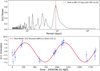 |
Fig. 1 Top panel: generalised Lomb-Scargle (GLS) periodogram of TOI-1611 b O–C transit times, with the best periodicity highlighted by a vertical red line. Bottom panel: O–C measurements over time, with the best-fitting sinusoidal model shown in red. |
3.1 Outlier rejection
Before searching for periodicity, we applied two filters to the O–C data to ensure robustness against outliers. First, we discarded any transit measurement whose error bars are excessively large (greater than 3 times the mean error). Second, we performed a 5-σ clipping on the O–C values themselves to remove any extreme timing outliers. Transits from sectors with long exposure times were in some cases (e.g. TOI-1516.01 and TOI-2046.01) considerably noisier6 than the rest and were thus excluded.
3.2 Periodicity search
We used the astropy.timeseries.LombScargle class (Astropy Collaboration 2013) to compute a frequency periodogram of the filtered O–C data, evaluated over the range f min ~ 1/(10ΔT) to f max ~ 1/(2Porb), where ΔT is the total baseline and Porb the orbital period. The periodicity search is only performed if a system has at least three valid transit measurements. The upper frequency limit corresponds to the effective Nyquist frequency of the transit sampling, ensuring that the periodogram includes all physically meaningful TTV signals within the data resolution. This naturally imposes a ‘Nyquist floor’ for TTVs, below which true variations cannot be reliably recovered; periods shorter than twice the orbital period would instead appear as aliases of the real modulation (Yahalomi et al. 2025). Within the physically defined bounds fmin and fmax, the detection efficiency mainly depends on the timing precision and the number of observed transits.
Figure 1 shows a sample periodogram for TOI-1611 b, highlighting the best periodicity and the corresponding false-alarm probability (FAP), together with the best-fitting sinusoid derived from that frequency.
3.3 Model selection and candidate classification
The core of our vetting process relies on a two-tiered statistical test to determine if a periodic TTV model is justified by the data. First, we compared the preferred sinusoidal model against a simple linear model (representing no TTVs or a secular trend). We use the Lomb-Scargle algorithm to find the best-fit sinusoid at the peak frequency, fTTV, considering both a single-term (N = 1) and double-term (N = 2) harmonic fit and selecting the one with the superior Bayesian information criterion (BIC). We then computed the ΔBIC between this best sinusoidal model and the linear model:
 (2)
(2)
A periodic model is considered strongly preferred only if ΔBIC ≥ 10 (Kass & Raftery 1995), indicating substantial evidence against a simple linear ephemeris.
Second, even if a periodic model is preferred, the signal must have a significant amplitude relative to the measurement uncertainties. We quantified this using a scatter statistic,  , which is defined as
 (3)
(3)
where MAD is the median absolute deviation, a robust estimator of the standard deviation (see, e.g., Holczer et al. 2016). This statistic measures the ratio of the observed scatter in the O–C data to the expected scatter from the median photometric timing precision, σO-C. Our targets are classified based on both criteria as listed below.
Strong candidates. The TTVs are significant, with both strong model preference (ΔBIC ≥ 10) and highly significant scatter (
 ).
).Weak candidates. Marginal detections with strong model preference (ΔBIC ≥ 10) but only moderate scatter (
 ).
).Non-detections. Cases where either the periodic model is not statistically preferred (ΔBIC < 10) or the timing scatter is consistent with the measurement errors (
 ).
).
We acknowledge that these thresholds are somewhat arbitrary and may differ in other studies; for transparency, we report the ΔBIC and  values for each system in Table A.1, and the full O–C list is available online, allowing follow-up studies to apply alternative criteria or select interesting targets for further investigations. We further note that the adopted thresholds could in principle introduce a bias against low signal-to-noise or long-period signals, where the statistical significance of a TTV pattern is harder to establish. Additional validation efforts, such as injection-recovery tests aimed at quantifying the detectability of synthetic TTV signals under realistic noise conditions, would help to characterise these effects more precisely, but performing such simulations would require significant computational resources and was therefore beyond the scope of this work.
4 Results
The analysis of our 423-system sample yields six and ten new candidates with strong and weak TTVs, respectively. For each of those, we generated a three-panel diagnostic plot to facilitate visual inspection and further study (Figs. 2, A.1, and A.2). The panels display (1) the phase-folded transit light curve, corrected for the measured TTVs to show the quality of the underlying transit fit, (2) the O–C diagram as a function of time, and (3) the O–C diagram phase-folded to the detected TTV period with the best-fit sinusoidal model overplotted, which highlights the periodic nature of the signal.
In addition, in Table A.1 we provide a comprehensive summary of the derived orbital and TTV parameters for every system in the survey. Other than the ΔBIC and  values, the table includes the TTV classification, the TTV period (PTTV), and semi-amplitude (ATTV) for candidates; and the updated parameters (Porb, T0, Rp/R*, etc.) for all targets. In some cases, such parameters differ from published values owing to the inclusion of many new transits. For instance, the orbital period of TOI-139b turns out to be ∼20 minutes longer than the one presented in Mistry et al. 2023, whereas for the peculiar planet TOI-1690.01/WD 1856+534 b, hosted by a white dwarf (Vanderburg et al. 2020), we find a lower impact parameter and planet-to-star radius ratio. Conversely, for targets significantly affected by flux contamination from nearby sources, the planet-to-star radius ratio may be slightly underestimated, as no additional dilution correction was applied beyond the default PDC-SAP adjustment based on the TESS Input Catalogue.
The results of the fits were visually inspected to assess both the quality of the transit modelling and the derived transit timing variations. While this inspection confirms that the fits are generally robust, obtaining extremely accurate TTV measurements is beyond the scope of this work, as it would require the individualised modelling of each system. For instance, certain systems with a large number of transits could benefit from a higher number of live points in the nested sampling procedure; in this study, we limited the number of live points to 1000 or 5000 depending on the number of transits (below and above 30, respectively) to reduce computation time. Some targets in our sample have also been observed from the ground or by other space missions, and a comprehensive TTV study should incorporate all available transits (see, e.g. the analysis of TOI-1227b TTVs in Almenara et al. 2024).
This approach prioritises a homogeneous, large-scale analysis, while leaving the detailed characterisation of individual systems for follow-up studies. Furthermore, we opted not to fit independent transit durations for each transit, both to reduce computation time and because individual TESS transits generally lack the photometric precision to accurately constrain them7, unlike Kepler ones (see, e.g. Boley et al. 2020; Kaye & Aigrain 2025). Indeed, to our knowledge, transit duration variations for TESS have been observed in very few cases (e.g. TOI-1338 Ab, where the variations are attributed to the misalignment between the planet’s orbit and the binary stars - Kostov et al. 2020).
4.1 Strong TTVs confirmed in earlier studies
Among the planets that we find to have significant TTVs, there are some that have already been reported in previous studies. Nevertheless, they were included in this survey because they are still listed as single-planet systems in ExoFOP8. The recovery of such systems highlights the robustness of our analysis and its consistency with earlier works, including those employing different methodologies:
TOI-199 b: a Saturn-type planet (Mb ∼ 0.17 MJup, Rb ∼0.81 RJup) orbiting a G9 V star on a relatively long ∼105 d period (Hobson et al. 2023). Its clear timing variations have been employed in the discovery paper to reveal the existence of an outer Saturn-mass planet (Mc ∼ 0.28 MJup) with an orbital period of ∼274 d.
TOI-2180 b: a long period Jupiter (P ∼ 260 d, Mb ∼2.8 MJup, Rb ∼ 1.0RJup) orbiting a slightly evolved G5V star (Dalba et al. 2022). Despite being observed in only three transits, clear TTVs have been reported (Dalba et al. 2024) that are possibly linked to an outer massive companion, consistent with the long-term trend seen in archival radial-velocity (RV) data.
TOI-2202b: a warm Jupiter (Mb ∼ 0.90 MJup, Rb ∼0.98 RJup) orbiting a K8V star every ∼ 11.91 d (Trifonov et al. 2021). The large TTVs of this planet (ATTV ∼ 100 min, P ∼ 750 d) have been used in the discovery paper to announce the presence of another Jupiter-mass planet (Mc ∼0.37 MJup) in a 2:1 MMR with TOI-2202 b. We note that the number of transits has tripled since then, and an updated N-body analysis would greatly benefit from this expanded data set.
TOI-2537b: a warm Jupiter (P ∼ 94 d, Mb ∼ 1.3 MJup, Rb ∼1.0RJup) hosted by a K3V star (Heidari et al. 2025). With only three available transits, the TTVs of this planet are evident and have already been reported in the discovery paper as being due to the interaction with an outer Jupiter-mass planet, TOI-2537 c, first discovered through RVs.
TOI-4562b: a young (<700Myr), very eccentric (e ∼ 0.76) temperate Jupiter (Mb ∼ 2.30 MJup, Rb ∼ 1.12 RJup) orbiting an F7 V star every ∼ 225 d (Heitzmann et al. 2023). Its large TTVs (ATTV ∼ 43 min, P ∼ 1700 d) have been linked to the presence of a second Jupiter-mass planet (Mc ∼ 5.8, MJup) orbiting with a period of ∼4000 d (Fermiano et al. 2024); this is the longest orbital period discovered to date via TTVs.
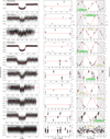 |
Fig. 2 Three-panel diagnostic plot for TTV candidates. Left: TTV-corrected, phase-folded transit light curve with the best-fit model. Middle: O–C measurements over time from first transit (t0, which is often, but not always, the same as T0 from Table A.1). Right: O–C diagram folded to best-fit TTV period (with the model represented by a dashed red line). The colour of the legend indicates the classification, with green and light yellow representing strong and weak candidates, respectively. Shaded regions indicate phase repetitions for visual continuity. |
4.2 Strong TTV candidates
We further identify six new strong candidates in our sample, as defined in Sect. 3.3, that, to our knowledge, have never been announced before. In particular:
TOI-120.01 / HD 1397 b: a moderately eccentric (e ∼ 0.25) warm Jupiter (M ∼ 0.41 MJup, R ∼ 1.03 RJup) orbiting a G-type subgiant with a period of ∼11.54 days (Nielsen et al. 2019). The transits of this planet display a possible modulation with P ∼ 42 d and ATTV = 4.3 minutes, though there are only 5 valid transits and more observations are needed to confirm the variation.
TOI-139 b: a sub-Neptune (R ∼ 2.46 R⊕) orbiting a K5 V star with a period of ∼11.07 d that has been statistically validated in Mistry et al. (2023). The planet has severe TTVs with semi-amplitude ≳11 hours and a long period (≳3500 d).
TOI-620b: a low-density, Neptune-sized planet (R ∼ 3.76R⊕ and M ≲ 7 M⊕ at 5σ confidence) transiting an M2.5V star with a period of ∼5.10 days (Reefe et al. 2022). Our analysis reveals variations with semi-amplitudes of ∼7 min on a timescale of ∼500 d. Given that the discovery paper reported a planet candidate with Porb ∼ 17.7 d, a careful follow-up of this target is warranted to assess whether the candidate could be responsible for the observed signal.
TOI-1611.01 / HD207897b: a sub-Neptune (R ∼ 2.46 R⊕, M ∼ 14.4 M⊕) orbiting a K0 V star with a period of ∼16.20 d (Heidari et al. 2022). Its transits show a variation with semiamplitude of ∼6.5 min and a plausible period of ∼900 d.
TOI-1859b: an eccentric (e ∼ 0.57) warm Jupiter (R ∼ 0.87 RJup) orbiting a F6V star on a misaligned orbit with period ∼63.48 d (Dong et al. 2023). The transits of this planet show a convincingly long TTV (P ∼ 2700 d) with semi-amplitude ∼9 min.
TOI-4495 b: a Neptune-sized planet (R ∼ 3.63 R⊕) orbiting an evolved F-type star with a period of ∼5.18 d, statistically validated in Hord et al. (2024). The planet shows clear TTVs (ATTV ∼ 75 min, P ∼ 2600 d) which may actually be related to a non-confirmed candidate in a 2:1 mean motion orbital resonance (MMR) with TOI-4495 b.
4.3 Additional noteworthy systems
Finally, we list a few candidates that did not pass the strong threshold criteria, though we still consider them worth mentioning:
TOI-1227b: a young (∼11 Myr) warm Jupiter (Rb ∼0.85 Rjup) orbiting a low-mass M5V star with an orbital period of ∼27.36 d (Mann et al. 2022). There are only five valid transits available, but one in particular is ∼50 min late and could signal the presence of a ∼300 d long TTV (
 , ΔBIC = 56.8). These variations have already been reported by Almenara et al. 2024, which suggested the presence of a 3:2 MMR ~6 M⊕ sub-Neptune. This points to the potential relevance of even our weaker candidates.
TOI-1742b: a moderately eccentric (e ∼ 0.3) sub-Neptune (M ∼ 9.7 M⊕, R ∼ 2.37 R⊕) orbiting a solar-type star every ∼21.27 d (Polanski et al. 2024). The transits show a periodic variation (P ∼ 775 d) with a semi-amplitude of ∼18 min. The large ΔBIC (~94) is offset by a modest
 , and the target is therefore classified as weak, though it still warrants further investigation.
TOI-1807 b: an ultra-short-period (∼0.55 d) super-Earth (M ∼ 2.6 M⊕, R ∼ 1.4 R⊕) orbiting a K3 V star (Nardiello et al. 2022). This planet is barely below the threshold for strong candidates, with
 and ΔBIC = 125, though it displays convincing TTVs with Aττv ∼ 8 min and P ∼450 d. However, because the transits are quite shallow, some residual scatter remains in the O-C diagram, suggesting that more careful studies are warranted.
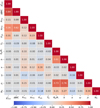 |
Fig. 3 Pearson correlation map of parameters listed in Table A.1 for all our sample. The Pearson coefficient, r, quantifies the strength and direction of linear relationships between pairs of variables (r = 1 and r = −1 indicate perfect positive and negative correlations, while r = 0 indicates no correlation). |
4.4 Correlation analysis
We computed the Pearson correlation (Pearson 1895) matrix of the key physical and statistical quantities of our sample to investigate which parameters drive the detectability of TTVs (Fig. 3). The analysis shows that TTV significance is primarily driven by the amplitude, ATTV, which correlates moderately with both  (r = 0.40) and ΔBIC (r = 0.43). Larger deviations thus yield more robust detections, unsurprisingly. The two significance metrics,
  and ΔBIC, are strongly correlated with each other (r = 0.84), validating their internal consistency as indicators of the presence of a signal.
Furthermore, the correlations among stellar density, impact parameter, and Rp/R* reflect parameter covariances in transit modelling. Even though ρ* is constrained by external priors, the degeneracy between b and Rp/R* propagates into the joint posterior, producing spurious trends (e.g. Sandford & Kipping 2017). In contrast, the positive correlation between eccentricity and orbital period reflects a genuine astrophysical trend that can be explained by tidal circularisation; close-in planets undergo orbital damping due to stellar tides, driving them towards circular orbits, whereas planets on wider orbits remain largely unaffected and retain their primordial eccentricities (Goldreich & Soter 1966; Rasio et al. 1996).
A more complex picture emerges when considering the orbital period. A weak positive trend is observed between Porb and  (r = 0.31), but this correlation vanishes when ΔBIC is considered (r = 0.03). This likely arises because long-period planets have fewer observed transits: although individual timing deviations can be substantial, the limited number of data points reduces the statistical significance once the increased model complexity is penalised by ΔBIC.
Finally, neither Rp/R* nor the eccentricity show any appreciable dependence on ΔBIC (r = −0.005 and r = −0.018, respectively). Overall, the statistical detectability of TTVs appears to be dictated only by the signal amplitude and likely driven by the system architecture alone, such as proximity to MMR.
5 Conclusions
We conducted a systematic and homogeneous TTV survey of 423 single-planet systems discovered by the TESS mission and already confirmed or validated by follow-up studies. We do not find any clear correlation between the presence or amplitude of TTVs and the physical or orbital properties of the transiting planets. This suggests that TTVs in our sample are primarily driven by the underlying system architecture, presumably by the proximity to MMR with unseen companions.
Within the scope of this survey, our main goal was to provide a well-motivated list of candidates for detailed follow-up. To achieve this, we employed a homogeneous methodology combining precise timing measurements from a GP-based Bayesian framework with a rigorous, two-tiered statistical test for candidate classification. This quantitative framework, which requires both strong model evidence (ΔBIC) and a significant scatter statistic ( ), ensures a high level of confidence in our strong candidates and will help increase the number of known multiplanet systems, with direct implications for demographic studies. While our analysis provides a uniform, large-scale assessment, we emphasise that individual systems may merit more detailed, case-by-case study; we therefore provide the full set of O–C values to allow others to explore or follow up targets of particular interest.
The results of this work, together with future follow-up efforts, pave the way for a deeper understanding of the architectures of planetary systems and the demographics of dynamically interacting systems discovered by TESS. The resulting catalogue of TTV candidates, along with their detailed diagnostic plots and summary parameters, offers a foundation for further work by the community. In particular, the strong candidates presented here should be considered prime targets for followup observations and for detailed N-body modelling to precisely determine the masses and orbits of any perturbing bodies. Looking ahead, a comprehensive TTV analysis of all TESS candidate planets (currently about 7500), in addition to the already confirmed multi-planet systems, could further contribute to the discovery of new planets and to a refined demographic picture. Such an effort, however, lies beyond the scope of this work, as it will require a substantially larger investment of time and resources.
Data availability
Table A.1 and the full O-C list are available at the CDS via https://cdsarc.cds.unistra.fr/viz-bin/cat/J/A+A/705/A5.
Acknowledgements
The author thanks the anonymous referee for their valuable comments and suggestions, which helped improve the quality of this manuscript. The author is also grateful to the colleagues at INAF - Osservatorio Astrofisico di Torino for helpful and stimulating conversations related to the TTV analysis. The author further acknowledges financial contribution from the INAF Large Grant 2023 “EXODEMO”. The present work has made extensive use of the 48-core HOT-ATMOS server at INAF - Osservatorio Astrofisico di Torino. This paper uses data from the TESS mission, whose funding is provided by the NASA Science Mission directorate. We acknowledge the use of the TESS archive, which is supported by the NASA Exoplanet Archive, and the ExoFOP-TESS service, which are operated by the California Institute of Technology, under contract with NASA. This work has made use of the Python packages numpy, pandas, matplotlib, lightkurve, dynesty, batman, astroquery, juliet and packages therein.
References
- Agol, E., Steffen, J., Sari, R., & Clarkson, W. 2005, MNRAS, 359, 567 [Google Scholar]
- Agol, E., Dorn, C., Grimm, S. L., et al. 2021, Planet. Sci. J., 2, 1 [NASA ADS] [CrossRef] [Google Scholar]
- Almenara, J. M., Bonfils, X., Guillot, T., et al. 2024, A&A, 683, A96 [NASA ADS] [CrossRef] [EDP Sciences] [Google Scholar]
- Alvarado-Montes, J. A., Sucerquia, M., Zuluaga, J. I., & Schwab, C. 2025, ApJ, 988, 66 [Google Scholar]
- Astropy Collaboration (Robitaille, T. P., et al.) 2013, A&A, 558, A33 [NASA ADS] [CrossRef] [EDP Sciences] [Google Scholar]
- Boley, A. C., Van Laerhoven, C., & Granados Contreras, A. P. 2020, AJ, 159, 207 [Google Scholar]
- Borucki, W. J., Koch, D., Basri, G., et al. 2010, Science, 327, 977 [Google Scholar]
- Christiansen, J. L., McElroy, D. L., Harbut, M., et al. 2025, Planet. Sci. J., 6, 186 [Google Scholar]
- Dalba, P. A., Kane, S. R., Dragomir, D., et al. 2022, AJ, 163, 61 [NASA ADS] [CrossRef] [Google Scholar]
- Dalba, P. A., Kane, S. R., Isaacson, H., et al. 2024, ApJS, 271, 16 [NASA ADS] [CrossRef] [Google Scholar]
- Dong, J., Wang, S., Rice, M., et al. 2023, ApJ, 951, L29 [NASA ADS] [CrossRef] [Google Scholar]
- Espinoza, N., Kossakowski, D., & Brahm, R. 2019, MNRAS, 490, 2262 [Google Scholar]
- Fausnaugh, M., Huang, X., Glidden, A., Guerrero, N., & TESS Science Office. 2018, AAS Meeting Abs., 231, 439.09 [Google Scholar]
- Fermiano, V., Saito, R. K., Ivanov, V. D., et al. 2024, A&A, 690, L7 [NASA ADS] [CrossRef] [EDP Sciences] [Google Scholar]
- Fernandes, R. B., Bergsten, G. J., Mulders, G. D., et al. 2025, AJ, 169, 208 [Google Scholar]
- Foreman-Mackey, D. 2018, Res. Notes Am. Astron. Soc., 2, 31 [NASA ADS] [Google Scholar]
- Goldreich, P., & Soter, S. 1966, Icarus, 5, 375 [Google Scholar]
- Guerrero, N. M., Seager, S., Huang, C. X., et al. 2021, ApJS, 254, 39 [NASA ADS] [CrossRef] [Google Scholar]
- Hadden, S., & Lithwick, Y. 2017, AJ, 154, 5 [Google Scholar]
- Harre, J.-V., Smith, A. M. S., Barros, S. C. C., et al. 2024, A&A, 692, A254 [NASA ADS] [CrossRef] [EDP Sciences] [Google Scholar]
- Heidari, N., Boisse, I., Orell-Miquel, J., et al. 2022, A&A, 658, A176 [NASA ADS] [CrossRef] [EDP Sciences] [Google Scholar]
- Heidari, N., Hébrard, G., Martioli, E., et al. 2025, A&A, 694, A36 [NASA ADS] [CrossRef] [EDP Sciences] [Google Scholar]
- Heitzmann, A., Zhou, G., Quinn, S. N., et al. 2023, AJ, 165, 121 [NASA ADS] [CrossRef] [Google Scholar]
- Hobson, M. J., Trifonov, T., Henning, T., et al. 2023, AJ, 166, 201 [NASA ADS] [CrossRef] [Google Scholar]
- Holczer, T., Mazeh, T., Nachmani, G., et al. 2016, ApJS, 225, 9 [Google Scholar]
- Holman, M. J., & Murray, N. W. 2005, Science, 307, 1288 [Google Scholar]
- Hord, B. J., Kempton, E. M. R., Evans-Soma, T. M., et al. 2024, AJ, 167, 233 [NASA ADS] [CrossRef] [Google Scholar]
- Ivshina, E. S., & Winn, J. N. 2022, ApJS, 259, 62 [CrossRef] [Google Scholar]
- Jenkins, J. M., Twicken, J. D., McCauliff, S., et al. 2016, SPIE Conf. Ser., 9913, 99133E [Google Scholar]
- Kass, R. E., & Raftery, A. E. 1995, J. Am. Stat. Assoc., 90, 773 [Google Scholar]
- Kaye, L., & Aigrain, S. 2025, MNRAS, 538, 2283 [Google Scholar]
- Kostov, V. B., Orosz, J. A., Feinstein, A. D., et al. 2020, AJ, 159, 253 [Google Scholar]
- Kreidberg, L. 2015, Astrophysics Source Code Library [record ascl:1510.002] [Google Scholar]
- Kunimoto, M., Winn, J., Ricker, G. R., & Vanderspek, R. K. 2022, AJ, 163, 290 [NASA ADS] [CrossRef] [Google Scholar]
- Lightkurve Collaboration (Cardoso, J. V. d. M., et al.) 2018, Astrophysics Source Code Library [record ascl:1812.013] [Google Scholar]
- Mann, A. W., Wood, M. L., Schmidt, S. P., et al. 2022, AJ, 163, 156 [NASA ADS] [CrossRef] [Google Scholar]
- Mazeh, T., Nachmani, G., Holczer, T., et al. 2013, ApJS, 208, 16 [Google Scholar]
- Mistry, P., Pathak, K., Prasad, A., et al. 2023, AJ, 166, 9 [NASA ADS] [CrossRef] [Google Scholar]
- Nardiello, D., Malavolta, L., Desidera, S., et al. 2022, A&A, 664, A163 [NASA ADS] [CrossRef] [EDP Sciences] [Google Scholar]
- Nielsen, L. D., Bouchy, F., Turner, O., et al. 2019, A&A, 623, A100 [NASA ADS] [CrossRef] [EDP Sciences] [Google Scholar]
- Pearson, K. 1895, Proc. R. Soc. London Ser. I, 58, 240 [Google Scholar]
- Polanski, A. S., Lubin, J., Beard, C., et al. 2024, ApJS, 272, 32 [NASA ADS] [CrossRef] [Google Scholar]
- Rasio, F. A., Tout, C. A., Lubow, S. H., & Livio, M. 1996, ApJ, 470, 1187 [Google Scholar]
- Reefe, M. A., Luque, R., Gaidos, E., et al. 2022, AJ, 163, 269 [NASA ADS] [CrossRef] [Google Scholar]
- Ricker, G. R., Winn, J. N., Vanderspek, R., et al. 2015, J. Astron. Telesc. Instrum. Syst., 1, 014003 [Google Scholar]
- Sandford, E., & Kipping, D. 2017, AJ, 154, 228 [NASA ADS] [CrossRef] [Google Scholar]
- Shahaf, S., Mazeh, T., Zucker, S., & Fabrycky, D. 2021, MNRAS, 505, 1293 [Google Scholar]
- Skilling, J. 2004, AIP Conf. Ser., 735, 395 [Google Scholar]
- Smith, J. C., Stumpe, M. C., Van Cleve, J. E., et al. 2012, PASP, 124, 1000 [Google Scholar]
- Speagle, J. S. 2020, MNRAS, 493, 3132 [Google Scholar]
- Stumpe, M. C., Smith, J. C., Van Cleve, J. E., et al. 2012, PASP, 124, 985 [Google Scholar]
- Stumpe, M. C., Smith, J. C., Catanzarite, J. H., et al. 2014, PASP, 126, 100 [Google Scholar]
- Trifonov, T., Brahm, R., Espinoza, N., et al. 2021, AJ, 162, 283 [NASA ADS] [CrossRef] [Google Scholar]
- Vanderburg, A., Rappaport, S. A., Xu, S., et al. 2020, Nature, 585, 363 [Google Scholar]
- Vanderspek, R., Huang, C. X., Vanderburg, A., et al. 2019, ApJ, 871, L24 [Google Scholar]
- Wang, W., Zhang, Z., Chen, Z., et al. 2024, ApJS, 270, 14 [NASA ADS] [CrossRef] [Google Scholar]
- Xie, J.-W., Wu, Y., & Lithwick, Y. 2014, ApJ, 789, 165 [NASA ADS] [CrossRef] [Google Scholar]
- Yahalomi, D. A., Kipping, D., Agol, E., & Nesvorný, D. 2025, ApJ, 984, L67 [Google Scholar]
- Yee, S. W., Winn, J. N., Knutson, H. A., et al. 2020, ApJ, 888, L5 [Google Scholar]
This should not be confused with the known-planet (KP) disposition, which designates planets identified prior to TESS by other facilities. In this work, we assumed that the CP transit dataset, unlike the KP one, is primarily composed of TESS observations.
We did not use the quick-look pipeline (QLP; Fausnaugh et al. 2018) light curves since SPOC products were available in most cases, and QLP data are generally noisier and less reliable (see, e.g. Appendix A of Fernandes et al. 2025). A proper use of QLP would require careful, system-by-system reduction, which was not appropriate for the automated, survey-wide approach adopted here.
For some systems, the 20-second cadence was also available, though the difference in transit time precision is often negligible, in comparison with the 2-minute cadence, while the increase in computational time was substantial.
Eccentricity was only allowed to vary when e > 0.1; otherwise, we fixed e = 0 and ω = 90°. For systems with truly small eccentricities, the transit shape is still accurately modelled, although the inferred stellar density may differ slightly from the real value to properly account for the transit duration.
The analyses were performed on an HPE ProLiant DL560 Gen10 rack server equipped with 2× Intel Xeon Gold 6252N processors (2.3 GHz, 24 cores, 150W each) and 128 GB of RAM, hosted at INAF - Osservatorio Astrofisico di Torino.
Longer exposures reduce temporal resolution, smoothing the ingress and egress and thus limiting the precision of the derived transit parameters. This effect is more pronounced for short-duration transits, while longer events remain well sampled and often benefit from the improved photometric stability of long-cadence data.
Typical transit duration variations observed in Kepler systems are of ~1 minute over several hundred days (Holczer et al. 2016; Shahaf et al. 2021), which is well below the average O–C uncertainty of ~5.8 minutes in our sample. Moreover, the irregular and often widely separated sector coverage of TESS further limits the detectability of such subtle duration changes.
The same is true for other systems with multiple confirmed transiting planets (e.g. TOI-1255) but no TTVs, since they were reported as single-planetary systems in ExoFOP.
Appendix A Additional figures and table
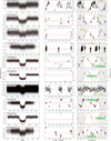 |
Fig. A.1 Continuation of Fig. 2. |
Summary of the TTV analysis results.
All Tables
All Figures
|
Fig. 1 Top panel: generalised Lomb-Scargle (GLS) periodogram of TOI-1611 b O–C transit times, with the best periodicity highlighted by a vertical red line. Bottom panel: O–C measurements over time, with the best-fitting sinusoidal model shown in red. |
| In the text | |
|
Fig. 2 Three-panel diagnostic plot for TTV candidates. Left: TTV-corrected, phase-folded transit light curve with the best-fit model. Middle: O–C measurements over time from first transit (t0, which is often, but not always, the same as T0 from Table A.1). Right: O–C diagram folded to best-fit TTV period (with the model represented by a dashed red line). The colour of the legend indicates the classification, with green and light yellow representing strong and weak candidates, respectively. Shaded regions indicate phase repetitions for visual continuity. |
| In the text | |
|
Fig. 3 Pearson correlation map of parameters listed in Table A.1 for all our sample. The Pearson coefficient, r, quantifies the strength and direction of linear relationships between pairs of variables (r = 1 and r = −1 indicate perfect positive and negative correlations, while r = 0 indicates no correlation). |
| In the text | |
|
Fig. A.1 Continuation of Fig. 2. |
| In the text | |
Current usage metrics show cumulative count of Article Views (full-text article views including HTML views, PDF and ePub downloads, according to the available data) and Abstracts Views on Vision4Press platform.
Data correspond to usage on the plateform after 2015. The current usage metrics is available 48-96 hours after online publication and is updated daily on week days.
Initial download of the metrics may take a while.