| Issue |
A&A
Volume 705, January 2026
|
|
|---|---|---|
| Article Number | A241 | |
| Number of page(s) | 10 | |
| Section | Galactic structure, stellar clusters and populations | |
| DOI | https://doi.org/10.1051/0004-6361/202557542 | |
| Published online | 26 January 2026 | |
Distribution of iron, oxygen, and sulfur in the direction of the outer arms of the Galaxy★
1
Astronomical Observatory, Odessa National University,
Shevchenko Park,
65014
Odessa,
Ukraine
2
Department of Physics and Astronomy, University of Hawai’i at Hilo,
Hilo,
HI
96720,
USA
3
Crimean Astrophysical Observatory,
Nauchny
298409,
Republic of Crimea
★★ Corresponding author: This email address is being protected from spambots. You need JavaScript enabled to view it.
Received:
3
October
2025
Accepted:
5
December
2025
Abstract
Aims. We conducted a high-resolution spectroscopic study of 51 distant Cepheids located in the outer part of the Galactic disk in the direction of the Perseus Arm. The aim of this investigation is to search for a possible observational manifestation of the influence of spiral arms or other dynamical processes on the chemical properties in this region of low-density gas.
Methods. The effective temperature for each Cepheid was obtained from the line-depth-ratio dependencies. Abundances of three chemical elements – oxygen, sulfur, and iron – were obtained. We used the local-thermodynamic-equilibrium (LTE) approximation for iron, and the nonlocal thermodynamic equilibrium (non-LTE) approximation for oxygen and sulfur.
Results. The abundances of iron, oxygen, and sulfur in our program stars were plotted as a function of galactocentric distances determined using heliocentric distances based on parallaxes from Gaia DR3, corrected for parallax bias. The Locally Weighted Scatterplot-Smoothing (LOWESS) method was used for statistical analysis of the plotted dependencies. We found a clear sign of flattening of the radial abundance distribution (plateau-like structure) for the studied elements, starting at a galactocentric distance of approximately 14 kpc. Formally dividing the overall iron abundance distribution into two parts and applying a linear regression for each section yields the following results on the gradient: –0.072 dex kpc−1 for the 8–14 kpc range and –0.006 dex kpc−1 for the 14–22 kpc range, with a formal intercept at 14 kpc. Similar gradients were also found for sulfur.
Conclusions. We believe this flattening is the result of the dynamical influence of the Perseus and other outer spiral arms on the global star formation processes in the gas disk at the outskirts of our Galaxy.
Key words: Galaxy: abundances
Based on observations obtained at the Canada–France–Hawaii Telescope (CFHT), which is operated by the National Research Council of Canada, the Institut National des Sciences de l’Univers of the Centre National de la Recherche Scientifique of France, and the University of Hawaii, and VLT archive spectra.
© The Authors 2026
 Open Access article, published by EDP Sciences, under the terms of the Creative Commons Attribution License (https://creativecommons.org/licenses/by/4.0), which permits unrestricted use, distribution, and reproduction in any medium, provided the original work is properly cited.
This article is published in open access under the Subscribe to Open model. This email address is being protected from spambots. You need JavaScript enabled to view it. to support open access publication.
1 Introduction
It is widely recognized that the radial and azimuthal abundance gradients in the Milky Way disk contain important information about its formation, structure and evolution. More generally, the global shape of the metallicity distribution (often parameter-ized by its slope), or any other specific features such as local variations or discontinuities (gaps), can provide significant information to further our understanding of the dynamical processes governing star formation and chemical evolution in galaxies, including our own. For the Milky Way, abundances derived from H II regions, planetary nebulae, open clusters, and stars and their radial distribution have been studied and modeled in great detail (e.g., Mollá et al. 2019). For this purpose, several research groups have focused on determining the elemental-abundance distribution across the Milky Way disk using high-resolution spectroscopy of a large number of Cepheids (e.g., Andrievsky et al. 2004; Martin et al. 2015; Genovali et al. 2015; Kovtyukh et al. 2019; da Silva et al. 2023; Trentin et al. 2023, and references therein). A detailed review of the Cepheid properties and their application to the Galaxy evolution study can be found, for example, in Bono et al. (2024).
As some studies have shown, large deviations of the stellar abundance gradient as a linear function are observed in the inner disk, particularly in the region adjacent to the Milky Way’s bar (e.g., Andrievsky et al. 2016), as well as at the periphery of the Galactic disk. Some studies have suggested wriggling in the iron radial-abundance distribution or a flattening in the abundance distribution in the outer disk beyond 11–13 kpc (e.g., Andrievsky et al. 2004, Korotin et al. 2014, and references therein). The peculiarity in the elemental-abundance distribution near 11–13 kpc could be related to the location of the Galaxy co-rotation resonance, which is defined as the radius of the circle around the Galactic center where the stellar component in the disk rotates at the same velocity as the spiral pattern. The spiral pattern rotates at a slower velocity than the stellar disk inside the co-rotation circle, while outside the co-rotation circle the rotation velocity is higher.
Several possible rotation characteristics of the Galaxy spiral pattern are discussed in the literature. Notably, numerous observational and theoretical studies have been conducted on identifying the exact location of the co-rotation resonance in the Galaxy. A complete review of the pattern-speed values obtained by various authors before 2001 can be found in Shaviv (2003). Bissantz et al. (2003) modeled the pattern angular velocity and found Ωp = 20 km s−1 kpc−1. Andrievsky et al. (2004) used a simple numerical model and considered two values for the kpc−1 and spiral pattern angular velocity: Ωp = 20 km s−1 kpc−1 and Ωp = 27 km s−1. The authors quantitatively compared the results of calculations with the observed metallicity distribution obtained from a large number of Cepheid spectra in the Galactic disk at galactocentric distances ranging from 4 to 16 kpc and favored the former value. In this case, the co-rotation resonance should be located at RG ≈ 11 kpc. More recent studies have shown, however, that the real situation may be more complex and that the value of the angular velocity may be a function of the galactocentric distance. The first evidence for this was provided by Naoz & Shaviv (2007). For example, these authors found that the Sagittarius–Carina Arm rotates with two angular velocities: about 17 km s−1 kpc−1 and 30 km s−1 kpc−1. For the Perseus Arm, they predicted 20 km s−1 kpc−1, while for the Local Arm this value is about 30 km s−1 kpc−1 (similar to the faster part of the Carina Arm). As recently reported by Castro-Ginard et al. (2021), the (four) different spiral arms exhibit different angular velocities, from about 50 to 20 km s−1 kpc−1. In particular, for the Perseus Arm, the authors give a pattern speed of about 18–21 km s−1 kpc−1 (see also a review of recent works on the topic in this paper). These results suggest that the angular velocity for the Scutum, Sagittarius, Local and Perseus Arms tends to decrease as RG increases (similarly to the Galactic-disk rotation curve). This conclusion was based on the study of the population of open clusters presented in Gaia Data Release 3 (DR3). More recently, Clarke & Gerhard (2022) investigated the distances and proper motions from the Infrared Astrometric Catalogue (VIRAC v1) and Gaia Data Release 2 and compared them with models. According to these authors, the angular velocity of the bar is approximately 33 km s−1 kpc−1. A similar conclusion was reached by Kawata et al. (2021). For the latter value, the radius of the co-rotation circle of the Milky Way is smaller and is about 7 kpc, while the outer Lindblad resonance is located at RG and of about 9 or 11–12 kpc (depending on the choice of the integer value of m – the number of spiral arms). An additional problem arises from the shape of the rotation curve of the Milky Way disk. For example, using the rotation curve from Roca-Fàbrega et al. (2014) a value of about 15 km s−1 kpc−1 for the angular velocity of the arms is needed in order to reach a distance of about 11 kpc for the co-rotation resonance position. However, Junqueira et al. (2015) used a sample of giant stars in open clusters and obtained a rotation velocity of 23 km s−1 kpc−1 for the pattern. Using open-cluster-population data from the Sagittarius–Carina, Local, and Perseus Arms, Dias et al. (2019) obtained a single, slightly higher value, namely 28 km s−1 kpc−1. As this brief overview shows, there is no complete consensus on the accepted values for the spiral pattern angular velocity within the Milky Way.
As discussed by Andrievsky et al. (2004), spiral arms should have an important influence on the star formation rate in the Galactic disk (of course, this has been explored previously in other works, but the star formation rate in Galactic chemody-namic models has typically been based on a power-law function of the local surface density of the gas in the disk, following the so-called Schmidt–Kennicutt law). At co-rotation, the velocity of the gas disk coincides with the velocity of the arms. Further away from the co-rotation, the relative velocity between the gas in the disk and the spiral arms becomes larger, leading to greater gas compression in the arm’s potential well, and it possibly results in a higher star formation rate. As a result, one can expect a larger number of Type II supernovae (SNe II) on both sides of the co-rotation circle and, consequently, a possibly higher rate of chemical enrichment of the interstellar gas with α- and iron-peak elements. A more sophisticated approach to studying the chemical evolution of the Milky Way was proposed by Spitoni et al. (2019), which presented a 2D model and described azimuthal variations in the Galactic-disk density (significant azimuthal variations in the oxygen abundance, which can be referred to as α elements). In short, based on several theoretical studies, one can expect to detect an increase in metallicity on either side of the co-rotation resonance, reflecting a local increase in the star formation rate and the corresponding production of chemical elements (primarily α elements) from SNe II.
The chemical properties of the Galactic disk regions toward the anticenter have not yet been studied in detail. This is evidenced, for example, by recent reviews presented by Bono et al. (2024), Fig. 28, adapted from da Silva et al. (2023); and Trentin et al. (2024), Fig. 9. The main questions that need to be answered in a detailed study of this region concern the dynamical influence of the distant parts of the spiral arms on the chemical properties of the disk, where the overall gas density gradually decreases; and how the possible presence of co-rotation resonance(s) in this region affect the nature of the metallicity distribution. In this paper, we aim to provide additional information based on our observational results, which may help in the future to resolve these and other questions regarding the chemodynamic evolution at the outskirts of our Galaxy.
2 Observations
Observations for 33 stars from our Cepheid sample were carried using the Echelle SpectroPolarimetric Device for the Observation of Stars (ESPaDOnS)1 at the 3.6-m Canada-France-Hawaii Telescope (CFHT) operated under the queue observing mode between 22 Oct 2023 and 5 Jan 2024 (UTC). One star had to be re-observed on 8 Apr 2025 because of a technical problem with the original data. The spectrograph was equipped with an e2v 2048 × 4608 CCD, used in its slow readout mode (readout noise ≈2.9 e−/pixel, binned 1 × 1), and was operated in the “star-only spectroscopy” observing configuration. The resolving power provided by this combination was about 80 000 with a spectral range extending from 370 to 1050 nm. Exposure times varied depending on the average magnitude of the Cepheid targeted. Typically, single exposures of 325 s (V ≈ 11) to 2200 s (V ≈ 13) were obtained while a few sequences of two consecutive exposures of 2200 s were gathered for the faintest objects (V ≈ 14) of our sample. Seeing during observations was mostly <1.5′′. The spectra were processed by the CFHT ESPaDOnS pipeline. The resulting estimated signal-to-noise ratio (S/N) at the continuum level depends upon the wavelength interval, but is in the range of 80–100 for each star.
We now discuss the VLT (Very Large Telescope). For part of our program, Cepheids we used archival spectroscopic data from the VLT Ultraviolet and Visual Echelle Spectrograph (UVES, Dekker et al. 2000)2. For these stars, typical exposure times of 1800–2700 seconds were performed per each object, with a 1′′ slit, resulting in a S/N ≈ 80. It should be noted that these spectra were previously analyzed by Trentin et al. (2023) and da Silva et al. (2023). The list of program stars and observation details are given in Table A.1.
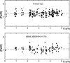 |
Fig. 1 Top: Control procedure of Teff determination using LDR method for V1016 Cas. Bottom: Effective temperature determination for ASAS J063519+2117.8, the only star for which the LDR method was not used. |
3 Method of analysis
3.1 Effective temperature, surface gravity, and microturbulent velocity
To determine the effective temperature of the program stars, we used a line-depth-ratio (LDR) method. This method assumes that the LDRs correlate with the effective temperature. For giant stars, 131 corresponding relationships between the LDRs and the effective temperature have been proposed, in particular by Kovtyukh (2007). These relations were revised and expanded, resulting in 257 relations obtained by Proxauf et al. (2018). Of these relations, 153 are found in the optical range for 11 chemical elements. The average effective temperature values obtained from all LDR relations have are fairly accurate (within several tens of Kelvins). For the stars sampled in our study, the number of LDR relations ranges from 15 to 92, depending on the star’s temperature and the S/N in the spectrum. The resulting average error on the effective temperature is less than 100 K. To verify the temperature values obtained from the LDR method, in some cases, we also used a standard procedure based on the dependence of the iron abundance derived from the Fe I lines and their lower level excitation potential. With the exception of one star (ASAS J063519+2117.8), the program stars demonstrated the independence of their iron abundance from the excitation potential. As for ASAS J063519+2117.8, we did not apply the LDR method, since its spectrum is contaminated by significant noise. We would like to emphasize that the standard procedure was considered only as a control method to exclude some unexpected results in the case of a limited number of LDRs. For the abundance analysis, we used the temperature values determined by the LDR method. As an illustration, Fig. 1 shows a plot of the iron abundance for two stars as a function of excitation potential with temperature values obtained with and without the help of the LDR method.
The surface gravity for each Cepheid was determined using the standard procedure of equalizing the iron-abundance values obtained separately from the Fe I and Fe II lines. Microturbulent velocity values for our stars were determined by avoiding any dependence between the iron abundance from each Fe I line and their equivalent widths (Fig. 2). The errors in determining the surface gravity and microturbulent velocity in our analysis do not exceed 0.2 dex and 0.15 km s−1, respectively.
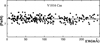 |
Fig. 2 Microturbulent-velocity determination for star V1016 Cas. Fe I lines are represented by circles, and asterisks are used for Fe II lines. Two linear approximations are shown. |
3.2 Iron, oxygen, and sulfur abundances
The iron abundance was determined under the LTE approximation. In fact, the non-LTE corrections for atoms with an iron-like structure of the energy levels are expected to be small (as shown by Bergemann et al. 2012 for red supergiants with solar-metallicity non-LTE corrections are less than ≈0.1 dex; for metal-poor stars corrections can be found in Koutsouridou et al. 2025). The non-LTE corrections for iron are obviously smaller (or comparable) than measurement errors and can be ignored in analysis.
Based on the Fe I and Fe II lines published by Jofré et al. (2014), Asplund et al. (2021) and da Silva et al. (2022) we generated a preliminary list of lines representing these two ionization stages. The selected lines were verified using the solar spectrum (Kurucz et al. 1984). We then used the DECH software (Galazutdinov 2022) to determine the equivalent widths of these lines. The oscillator strengths were taken from the Vienna Atomic Line Database (VALD, Ryabchikova et al. 2015) and NIST (Reader et al. 2012). Using these data, we determined the iron abundances with the help of the STARSP software (Tsymbal 1996). We adopted the value of (Fe/H)=7.51 for the solar iron abundance (Lodders et al. 2025). Finally, we generated the line lists for Fe I (303 lines) and Fe II (59 lines). These lines were selected such that the difference between the iron abundance derived from these two ionization stages and the adopted value of 7.51 did not exceed 0.1 dex.
For our spectroscopic analysis, we only used the infrared lines of neutral oxygen (7771–7775 Å and 8446 Å). The O I level populations were determined using the MULTI software developed by Carlsson (1986) with modifications by Korotin et al. (1999). As mentioned in our previous papers, a correct comparison of the observed and calculated oxygen line profiles usually requires a multielement spectral synthesis to account for possible blending lines form other species. For this process, we combined non-LTE (MULTI code) calculations (specifically, the departure coefficients b = Nnon−LTE/NLTE) with the local-thermodynamic-equilibrium (LTE) synthetic spectrum software SynthV (Tsymbal et al. 2019), which allowed us to calculate the non-LTE source function and the opacity for oxygen lines. These calculations included all spectral lines from the VALD database (Ryabchikova et al. 2015) in the region of interest. The LTE approximation was applied to lines other than the O I lines. The abundances of the corresponding chemical elements were taken according to the [Fe/H] values for each Cepheid. It should be noted that this approach is not very important for the infrared oxygen lines, which are not significantly blended.
The oxygen atom model used in our non-LTE calculations was first described in Mishenina et al. (2000) and later updated by Korotin et al. (2014). The model consists of 51 O I levels of singlet, triplet, and quintet systems, as well as the ground level of the O II ion. An additional 24 levels of neutral oxygen and 15 levels of ions O II and O III were added for particle number conservation. Fine structure splitting was taken into account only for the ground level and the 3p 5P level (the upper level of the 7771–7775 Å triplet lines). In total, 248 bound–bound transitions were taken into consideration. Accurate quantum-mechanic calculations were employed for the first 19 levels to find the collision rates with electrons (Barklem 2007). Inelastic processes in oxygen–hydrogen collisions were taken into account for the first 13 levels O I (Belyaev et al. 2019). The infrared triplets 7771–7775 Å and 8446 Å show the largest non-LTE effects. Oxygen abundance was not derived for the stars observed with VLT because the infrared oxygen lines are out of the spectral range. Fig. 3 shows a comparison between the observed and calculated profiles of the infrared O I lines for one Cepheid of our program.
Following the works of da Silva et al. (2023) and Bono et al. (2024), we also determined the sulfur abundance in our program’s Cepheids. Sulfur, as α elements, is formed in SNe type II explosions. To determine the sulfur abundance in the non-LTE approximation, we used the sulfur atomic model first described in Korotin (2009) and later modified by Korotin & Kiselev (2024). We considered 64 energy levels for neutral sul-fur, 81 levels for ionized sulfur and the ground level for the ion S III. In addition, to more fully account for the number of particles requiring conservation, we included one level of S I, six levels of S III, and the ground level of S IV, for which the populations were calculated in LTE. The fine structure of the levels was not taken into account. A total of 775 bound–bound and 146 bound–free transitions between levels were considered. Unlike the previous version of the sulfur atomic model (Korotin 2009), which used approximation formulas to account for collisions with electrons and hydrogen atoms, this model uses quantum mechanical calculations (Belyaev & Voronov 2020; Tayal & Zatsarinny 2010; Summers & O’Mullane 2011). Similarly to oxygen, the level populations in the sulfur atom were obtained with the help of MULTI software (Carlsson 1986, version 2.3). As usual, the resulting b-factors were then included in the program of the synthetic spectrum calculation SynthV (Tsymbal et al. 2019), where they are used to calculate the sulfur line profiles taking into account non-LTE effects, while the lines of other elements in the region of interest were calculated in the LTE approximation. All line parameters used to calculate the synthetic spectrum were taken from the VALD (Ryabchikova et al. 2015), similarly to what was done for oxygen. To determine the sulfur abundance, we used the following multiplets of SI: the first (9212 Å and 9237 Å), the sixth (8694 Å), the eighth (6743–6757 Å), and the tenth (6052 Å). It should be noted that the lines of the eighth and tenth multiplets consist of three lines each, and each of these lines is a superposition of three components with a small shift in wavelength. The shape of the line of these multiplets is far from a Gaussian profile, so calculating a synthetic spectrum is absolutely necessary when comparing with the observed profiles. For the VLT spectra of our program stars, the accessible region reaches only 6800 Å, so for these spectra we only analyzed the lines of the eighth and tenth multiplets. Fig. 4 shows a comparison between the observed and calculated sulfur line profiles.
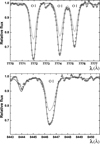 |
Fig. 3 Comparison of observed (open circles) and calculated (non-LTE, continuous line) profiles of oxygen infrared lines for ASAS J052610+1151.3. Profiles calculated in LTE with the same abundance that was used to fit the observed and calculated non-LTE profiles are shown by the dashed line. |
4 Results of spectroscopic analysis
4.1 Distances
The best approach in determining heliocentric distances for our program’s (pulsating) Cepheids would be to use the period– luminosity relation. However, according to the literature, some of our objects (observed with CFHT) pulsate in overtone modes. If the mode identification is questionable, the period–luminosity relation yields an incorrect distance. Therefore, we first decided to estimate distances based on the parallaxes provided by Gaia DR3. For this, we used the extensive Cepheid data collected by Luck (2018). Luck (2018) used distances obtained from Gaia DR2 parallaxes. Fig. 9 of his paper shows that the distance data based on Gaia DR2 are not entirely reliable. Distances based on the Gaia DR3 parallaxes (SIMBAD) should be more accurate (Figs. 5 and 6). However, there is evidence that distances obtained by the direct inversion of the Gaia parallaxes are biased. This is a compelling argument for introducing a correction to the Gaia DR3 parallaxes. This was done according to the recipe recently proposed by Lindegren et al. (2021). For this, we used the Gaia G magnitudes of our program’s stars and their (Bp–Rp) colors (SIMBAD). Using the color values, we determined the effective wave number νeff for each star using relation (1) from that paper. The bias function Z5(G,νeff, β), where β is the ecliptic latitude of each sample star, was calculated and then subtracted from each individual Gaia DR3 parallax value. The parallaxes thus corrected were used to obtain heliocentric distances of our program stars (Table A.1), and stars from Luck’s sample.
It should be noted that several stars from the Luck sample were excluded from consideration (AU Peg, BC Aql, DD Vel, EK Del, EV Aql, FQ Lac, GT Aur, HK Cas, QQ Per, V484 Mon, V526 Aql, V1359 Aql, SU Cru, Y Mon). For example, QQ Per and DD Vel belong to the W Vir type stars (General Catalogue of Variable Stars, GCVS and SIMBAD). Moreover, this classification for QQ Per was confirmed by Wallerstein et al. (2008), who noted a strong Hα emission at the early phases of the pulsation cycle. A similar classification is given in SIMBAD for AU Peg and V526 Aql, while V1359 Aql according to GCVS, is an SRD variable (semi-regular, of type d). Soszyński et al. (2020) classified V484 Mon as a pulsating variable of BL Her type. The extremely metal-deficient star BC Aql (compared to classical Cepheids) is in fact a T2Cs (BL Her type) object. Y Mon is the Mira variable (GCVS, SIMBAD). For the rest of the sample of problematic objects, the question of their correct classification remains open.
To determine the galactocentric distances for the Cepheids in our program, we used the well-known equation
 where RG,⊙ is the galactocentric distance of the Sun (8.178 kpc, as recommended by the GRAVITY Collaboration 2019).
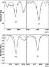 |
Fig. 4 Comparison of observed (open circles) and calculated (non-LTE, continuous line) profiles of sulfur lines for GI CMa. Profiles calculated in LTE with the same abundance that was used to fit the observed and calculated non-LTE profiles are shown by the dashed line. |
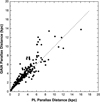 |
Fig. 5 Comparison of distances obtained using the period–luminosity relation (Madore et al. 2017) and Gaia DR3 parallax distances. |
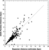 |
Fig. 6 Comparison of distances from Bailer-Jones et al. (2018) and Gaia DR3 parallax distances. |
4.2 Iron-, oxygen-, and sulfur-abundance distributions
Some of the fundamental characteristics of the Cepheids included in our sample, their elemental abundances, as well as their respective calculated galactocentric distance, are given in Table A.2. Fig. 7 shows the distribution of iron, oxygen, and sulfur abundances in our program’s stars as a function of the galactocentric distance. To fit the observed data, we used the locally weighted scatterplot-smoothing (LOWESS) polynomial regression method. It works by fitting simple polynomial models to localized subsets of the data, taking into account a weight for each point, where nearby points receive more weight. For oxygen, the observational data are less complete, while for sul-fur and iron the situation is better, allowing us to conclude that the distributions flatten out at approximately 14 kpc. This is also clearly visible in Fig. 8, where we combined our data with those of Luck (2018); see text above. At least two unusual regions can be noted in the iron-abundance-distribution plot. One is located at about 7–10 kpc, and another is at around 14 kpc and extends further into the outer disk.
To localize our sample of Cepheids observed in the Galactic disk for this study, we used a model of the spiral-arm structure published by Reid et al. (2019). A similar picture is also provided by mapping the perturbed surface density of the neutral hydrogen (Levine et al. 2006). The locations of our program’s Cepheids relative to the Galaxy outer arms are shown in Fig. 9.
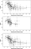 |
Fig. 7 Iron, oxygen and sulfur abundance distributions for our program stars as a function of galactocentric distance. The interval 2-σ is indicated. |
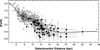 |
Fig. 8 Iron abundance distribution as function of galactocentric distance (our program stars – filled circles; Luck 2018 – open circles). |
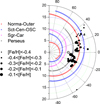 |
Fig. 9 Position of Cepheid stars observed in our study shown relative to the location of the main Galactic spiral arms (Reid et al. 2019). The radial galactocentric distance is displayed in kiloparsecs. The position of the Sun is indicated by the ⊙ symbol. |
5 Discussion
The very first use of Cepheids for qualitatively assessing the chemical composition in the Galaxy was made by van den Bergh (1958), which used stars with different pulsation periods for this purpose. The first comprehensive study of the elemental abundance distributions (25 chemical elements) and the Galactic abundance gradient using high-resolution spectroscopic data on 77 Galactic Cepheids was initiated by Andrievsky et al. (2002b). This study used fairly reliable distances to the Cepheids based on the period–luminosity relation, which is critical for determining the radial-abundance gradient. Later, Andrievsky et al. (2002a), Andrievsky et al. (2002c), and Luck et al. (2003) conducted a more detailed study of the abundance distributions in the intermediate and outer parts of the Galactic disk. These results were summarized by Andrievsky et al. (2004). The authors also used a simple model for the Galactic chemical evolution based on the instantaneous recycling approximation, which is more applicable to the yield of oxygen and α elements than to iron, the formation of which is also significantly affected by long-lived, low-mass stars associated with Type I supernovae. However, the authors used extensive iron-abundance data from their Cepheid sample, along with α-element abundances.
A simple Galactic chemodynamical model showed that the better agreement between the observed abundance distribution and model prediction is achieved at a Galactic co-rotation radius of approximately 11 kpc. Since the gaseous disk within the co-rotation circle rotates faster than the spiral pattern, and the opposite is true outside the co-rotation circle, the relative velocity between the gas disk and the spiral arms on either side of the co-rotation circle is expected to be higher than on the co-rotation circle itself, where the relative velocity is close to zero. Consequently, regions of the Galactic disk far from the co-rotation circle make an additional contribution to the star formation. In simple terms, the further away it is from the co-rotation circle, the more efficient the star formation process and, hence, the yield of certain chemical elements, are. Given that the total metallicity (corresponding to the gas density) decreases exponentially from the inner to the outer regions of the Galactic disk, it can be assumed that the additional contribution to the metal content within the co-rotation circle will be less noticeable than for the zone on the other side of the circle. This may lead to some flattening of the abundance distribution in the region of the disk outside the co-rotation circle. Such flattening can be suggested for the iron- and sulfur-abundance distributions (Figs. 7 and 8), while data on the oxygen abundance in distant stars are scarce.
As mentioned in the introduction, Bono et al. (2024) recently discussed the properties of Cepheids in detail. In connection with this fundamental work, the most recent relevant papers of da Silva et al. (2023) (Cepheids and open clusters), Trentin et al. (2024), and Minniti et al. (2020) can be mentioned (see also references therein). In these works, the elemental abundance gradient in the Galactic disk was studied (with particular attention paid to the distant Cepheids). Here, we briefly review the results of the linear fit to the iron abundance distribution reported by these authors. They are as follows. Minniti et al. (2020): gradient −0.062 ± 0.013 dex kpc−1, studied range (≈4– 23 kpc); Trentin et al. (2024): −0.064 ± 0.003 (≈5–20 kpc); da Silva et al. (2023): −0.041 ± 0.03 (≈5–17 kpc). The latter work also examined the more distant Cepheids, and the abundance distribution including these stars shows some smoothing or flattening (a cautious conclusion about smoothing was also made by Minniti et al. 2020, but their data on distant Cepheids are sparse). As mentioned above, Figs. 7 and 8 show our results from fitting abundance distributions using the LOWESS method. Clearly, it is impossible to describe the constructed abundance distributions of each chemical element using a single gradient value. For the quantitative description of the spatial behavior of the abundance gradient, we divided these distributions into several distinct regions and performed linear interpolations within each of these regions. In Fig. 7, we show the following: iron-abundance gradient = −0.072 dex kpc−1, range (≈8–14 kpc); −0.006 dex kpc−1, (≈14–22 kpc); oxygen-abundance gradient = −0.052 dex kpc−1, range (≈8–14 kpc); sulfur-abundance gradient = −0.078 dex kpc−1, range (≈8–14 kpc); −0.007 dex kpc−1, range (≈14–22 kpc). Fig. 8 shows the following: iron-abundance gradient = −0.152 dex kpc−1, range (≈4–7 kpc); −0.038 dex kpc−1, range (≈7–10.5 kpc); −0.071 dex kpc−1, range (≈10.5–13.5 kpc); −0.004 dex kpc−1, range (≈13.5–25 kpc). A comparison of the iron gradient obtained only for our data in the range from 8 to 14 kpc (Fig. 7) shows that we are in satisfactory agreement with the gradient values obtained by Minniti et al. (2020) and Trentin et al. (2024). We are also in agreement with da Silva et al. (2023), except for the 7–11 kpc range in Fig. 8. Earlier studies (e.g., Genovali et al. 2014) also reported a gradient value similar to ours of −0.060 dex kpc−1 for the range of galactocentric distances of 5–19 kpc, although their Fig. 4 suggests some smoothing of the iron-abundance distribution starting at approximately 12 kpc.
The flattening of the radial abundance gradient in the outer parts of the Milky Way may be a sign of some chemodynamic processes at play in this region. One of the possible mechanisms responsible for the observed discontinuity/local variation in the elemental-abundance distribution could be the dynamic influence of the co-rotation resonance. This hypothesis is supported by the results of Castro-Ginard et al. (2021), Fig. 5, which shows the pattern velocity distribution across the disk for different spiral arms (a multimodal pattern of velocity distribution) along with the disk rotation curve. If we roughly extrapolate the pattern speed for the Perseus Arm, the intersection with the rotation curve should be at a galactocentric distance of approximately 13 kpc. Esteban et al. (2013) also found a flattening in the distribution of oxygen, carbon, and nitrogen after analyzing the Galactic H II region NGC 2579, located at approximately 12 kpc (see their Fig. 4). A similar conclusion but for a large sample of the H II regions (7000 regions from 306 galaxies) can be drawn from the results of Sánchez et al. (2014), Fig. 9; radial oxygen-abundance distribution after scaling to the average value at the disk effective radius for each galaxy is given in that figure.
It cannot be excluded that the fast rotating outer spiral arms trigger a more efficient star formation process in the disk, i.e., more efficient than the star formation determined by the surface density of the gaseous disk (Schmidt–Kennicutt law), since the gas density of the outer parts of the disk should be significantly reduced. At the outskirts of the Galactic disk, the usual exponential regime (approximately linear on a logarithmic scale) of metallicity decrease is replaced by a plateau-like distribution. Secondary processes may also play a certain role. For example, as noted by Reid et al. (2014), the width of the spiral arms increases with distance from the Galactic center and can reach about 600 pc at a distance of about 15 kpc, which is of the same order of magnitude as the inter-arm distance. Along with this factor, one can also consider the migration or spatial scattering of stars caused by the arms (e.g., Mishurov & Acharova 2011). These processes can smooth out the metallicity over a large area. Thus, it can be hypothesized that the plateau-like structure in the metallicity distribution may be the result of the combined effect of the effective additional yield of chemical elements from the Perseus and other outer arms (as well as possible yet unknown arm-like structures between them, the presence of which can be assumed, as shown by Reid et al. 2014, their Fig. 1). It is possible that some more distant arm-like structures are also involved in this process (Reid et al. 2019, Fig. 2), if the outer Lindblad resonance is located far enough in the Galactic disk. Of course, other scenarios exist to explain the discontinuity of the linear distribution seen in the Galaxy outskirts. For instance, models of the Galaxy abundance gradient developed by Mollá et al. (2019) support the hypothesis that inflows of enriched gas from active star formation regions in the halo might have contributed to flattening the abundance distribution. Other dynamic structures such as the Galaxy bar might have redistributed enriched material from the inner parts in the disk to the outskirts as well (e.g., Vera et al. 2016; Zurita et al. 2021).
6 Summary
In the present study, we performed a quantitative spectroscopic analysis of 51 distant Cepheids, observed with high-resolution spectrographs at CFHT and the VLT, located in the region close to the Perseus Arm and other outer arms of the Galaxy. The stellar atmosphere parameters and iron abundance in these stars were determined using the LDR method (effective temperature) and a list of carefully checked iron lines. The oxygen and sul-fur abundances in our program Cepheids were obtained using the non-LTE approach. Only infrared oxygen lines were used. Unfortunately, these lines are not available from the VLT spectra, so the oxygen-abundance distribution remains poorly sampled at large galactocentric distances.
By combining our data with data from the extensive study of Luck (2018), we performed a LOWESS fit to the elemental-abundance distribution over the galactocentric distance and found a clear sign of flattening at the distances greater than approximately 14 kpc. A similar flattening of the O/H abundance gradient in the gas phase has been reported in the outskirts of many spiral galaxies (e.g., Sánchez et al. 2014), including the Milky Way (Esteban et al. 2013). However, there is considerable doubt surrounding this conclusion for many objects as the uncertainties and systematic errors related to the methods used in deriving nebular abundances are large. As stated above, the flattening was also mentioned in the Cepheid studies (e.g., da Silva et al. 2023, Minniti et al. 2020). We consider this apparent flattening in the Cepheid iron and sulfur abundances in the Milky Way outskirts to be the possible result of the combined dynamic effects from the outer spiral arms (Perseus, Norma– Outer, Scutum–Centaurus, and possible inter-arm structures), effectively increasing the metallicity level where the gas density is expected to be low. Using the LOWESS method of statistical analysis, we show that flattening starts at a galactocentric distance of about 14 kpc, and this radius can mark the position of the co-rotation circle. Despite supporting prior studies reporting a flattening in the abundance gradient in the outer disk of the Galaxy as mentioned earlier, and considering that available heliocentric distances for some program stars may not be accurate and that the abundances for distant faint stars can be less reliable, we regard our conclusion as preliminary. Additional surveys of abundances in a large sample of stars located in the Galaxy outskirts will be needed to confirm our results.
The future role of the Cepheids in such studies of the dynamical and chemical properties of spiral arms is difficult to overestimate. Cepheids offer several undeniable advantages over other objects used to determine the elemental-abundance gradient in the Galactic disk. These stars serve as reliable distance calibrators. Cepheids are luminous stars, allowing us to study the distant regions of the disk. The abundances of many chemical elements can be inferred from the Cepheid spectra, including the non-LTE abundances. Cepheids are relatively young, massive stars, which have not had enough time to move far from their birthplaces, so they can serve as excellent indicators of the present-day metallicity in the Galacic disk. Further verification of the flattening effect reported here and in some other works is necessary with larger scale spectroscopic surveys of distant Cepheids.
Acknowledgements
We are pleased to thank the referee for his/her positive assessment of this study and comments, which undoubtedly improved this paper. We are also grateful to the queue observing team at the Canada-France-Hawaii Telescope for performing the observations for 31 Cepheids of this program. The authors wish to recognize and acknowledge the very significant cultural role that the summit of Mauna Kea has always had within the indigenous Hawaiian community. We are most grateful to have the opportunity to conduct observations from this mountain. The authors would also like to acknowledge Dr. V. Kov-tyukh, with whom we began work on the first stage of this project. This research has made use of the SIMBAD database, operated at CDS, Strasbourg, France.
References
- Andrievsky, S. M., Bersier, D., Kovtyukh, V. V., et al. 2002a, A&A, 384, 140 [NASA ADS] [CrossRef] [EDP Sciences] [Google Scholar]
- Andrievsky, S. M., Kovtyukh, V. V., Luck, R. E., et al. 2002b, A&A, 381, 32 [NASA ADS] [CrossRef] [EDP Sciences] [Google Scholar]
- Andrievsky, S. M., Kovtyukh, V. V., Luck, R. E., et al. 2002c, A&A, 392, 491 [NASA ADS] [CrossRef] [EDP Sciences] [Google Scholar]
- Andrievsky, S. M., Luck, R. E., Martin, P., & Lépine, J. R. D. 2004, A&A, 413, 159 [NASA ADS] [CrossRef] [EDP Sciences] [Google Scholar]
- Andrievsky, S. M., Martin, R. P., Kovtyukh, V. V., Korotin, S. A., & Lépine, J. R. D. 2016, MNRAS, 461, 4256 [NASA ADS] [CrossRef] [Google Scholar]
- Asplund, M., Amarsi, A. M., & Grevesse, N. 2021, A&A, 653, A141 [NASA ADS] [CrossRef] [EDP Sciences] [Google Scholar]
- Bailer-Jones, C. A. L., Rybizki, J., Fouesneau, M., Mantelet, G., & Andrae, R. 2018, AJ, 156, 58 [Google Scholar]
- Barklem, P. S. 2007, A&A, 462, 781 [NASA ADS] [CrossRef] [EDP Sciences] [Google Scholar]
- Belyaev, A. K., & Voronov, Y. V. 2020, ApJ, 893, 59 [NASA ADS] [CrossRef] [Google Scholar]
- Belyaev, A. K., Voronov, Y. V., Mitrushchenkov, A., Guitou, M., & Feautrier, N. 2019, MNRAS, 487, 5097 [CrossRef] [Google Scholar]
- Bergemann, M., Kudritzki, R.-P., Plez, B., et al. 2012, ApJ, 751, 156 [Google Scholar]
- Bissantz, N., Englmaier, P., & Gerhard, O. 2003, MNRAS, 340, 949 [NASA ADS] [CrossRef] [Google Scholar]
- Bono, G., Braga, V. F., & Pietrinferni, A. 2024, ARA&A Rev., 32, 4 [Google Scholar]
- Carlsson, M. 1986, Uppsala Astronomical Observatory Reports, 33 [Google Scholar]
- Castro-Ginard, A., McMillan, P. J., Luri, X., et al. 2021, A&A, 652, A162 [NASA ADS] [CrossRef] [EDP Sciences] [Google Scholar]
- Clarke, J. P., & Gerhard, O. 2022, MNRAS, 512, 2171 [NASA ADS] [CrossRef] [Google Scholar]
- da Silva, R., Crestani, J., Bono, G., et al. 2022, A&A, 661, A104 [NASA ADS] [CrossRef] [EDP Sciences] [Google Scholar]
- da Silva, R., D’Orazi, V., Palla, M., et al. 2023, A&A, 678, A195 [NASA ADS] [CrossRef] [EDP Sciences] [Google Scholar]
- Dekker, H., D’Odorico, S., Kaufer, A., Delabre, B., & Kotzlowski, H. 2000, SPIE Conf. Ser., 4008, 534 [Google Scholar]
- Dias, W. S., Monteiro, H., Lépine, J. R. D., & Barros, D. A. 2019, MNRAS, 486, 5726 [NASA ADS] [CrossRef] [Google Scholar]
- Esteban, C., Carigi, L., Copetti, M. V. F., et al. 2013, MNRAS, 433, 382 [NASA ADS] [CrossRef] [Google Scholar]
- Galazutdinov, G. A. 2022, Astrophys. Bull., 77, 519 [Google Scholar]
- Genovali, K., Lemasle, B., da Silva, R., et al. 2015, A&A, 580, A17 [NASA ADS] [CrossRef] [EDP Sciences] [Google Scholar]
- Genovali, K., Lemasle, B., Bono, G., et al. 2014, A&A, 566, A37 [NASA ADS] [CrossRef] [EDP Sciences] [Google Scholar]
- GRAVITY Collaboration (Abuter, R., et al.) 2019, A&A, 625, L10 [NASA ADS] [CrossRef] [EDP Sciences] [Google Scholar]
- Jofré, P., Heiter, U., Soubiran, C., et al. 2014, A&A, 564, A133 [NASA ADS] [CrossRef] [EDP Sciences] [Google Scholar]
- Junqueira, T. C., Chiappini, C., Lépine, J. R. D., Minchev, I., & Santiago, B. X. 2015, MNRAS, 449, 2336 [Google Scholar]
- Kawata, D., Baba, J., Hunt, J. A. S., et al. 2021, MNRAS, 508, 728 [NASA ADS] [CrossRef] [Google Scholar]
- Korotin, S. A. 2009, Astron. Rep., 53, 651 [Google Scholar]
- Korotin, S. A., & Kiselev, K. O. 2024, Astron. Rep., 68, 1159 [Google Scholar]
- Korotin, S. A., Andrievsky, S. M., & Luck, R. E. 1999, A&A, 351, 168 [NASA ADS] [Google Scholar]
- Korotin, S. A., Andrievsky, S. M., Luck, R. E., et al. 2014, MNRAS, 444, 3301 [NASA ADS] [CrossRef] [Google Scholar]
- Koutsouridou, I., Skúladóttir, Á., & Salvadori, S. 2025, A&A, 699, A32 [NASA ADS] [CrossRef] [EDP Sciences] [Google Scholar]
- Kovtyukh, V. V. 2007, MNRAS, 378, 617 [NASA ADS] [CrossRef] [Google Scholar]
- Kovtyukh, V., Lemasle, B., Kniazev, A., et al. 2019, MNRAS, 488, 3211 [Google Scholar]
- Kurucz, R. L., Furenlid, I., Brault, J., & Testerman, L. 1984, Solar Flux Atlas from 296 to 1300 nm (National Solar Observatory Atlas, Sunspot, New Mexico: National Solar Observatory) [Google Scholar]
- Levine, E. S., Blitz, L., & Heiles, C. 2006, Science, 312, 1773 [NASA ADS] [CrossRef] [Google Scholar]
- Lindegren, L., Bastian, U., Biermann, M., et al. 2021, A&A, 649, A4 [EDP Sciences] [Google Scholar]
- Lodders, K., Bergemann, M., & Palme, H. 2025, Space Sci. Rev., 221, 23 [Google Scholar]
- Luck, R. E. 2018, AJ, 156, 171 [Google Scholar]
- Luck, R. E., Gieren, W. P., Andrievsky, S. M., et al. 2003, A&A, 401, 939 [NASA ADS] [CrossRef] [EDP Sciences] [Google Scholar]
- Madore, B. F., Freedman, W. L., & Moak, S. 2017, ApJ, 842, 42 [NASA ADS] [CrossRef] [Google Scholar]
- Martin, R. P., Andrievsky, S. M., Kovtyukh, V. V., et al. 2015, MNRAS, 449, 4071 [NASA ADS] [CrossRef] [Google Scholar]
- Minniti, J. H., Sbordone, L., Rojas-Arriagada, A., et al. 2020, A&A, 640, A92 [EDP Sciences] [Google Scholar]
- Mishenina, T. V., Korotin, S. A., Klochkova, V. G., & Panchuk, V. E. 2000, A&A, 353, 978 [NASA ADS] [Google Scholar]
- Mishurov, Y. N., & Acharova, I. A. 2011, MNRAS, 412, 1771 [Google Scholar]
- Mollá, M., Díaz, Á. I., Cavichia, O., et al. 2019, MNRAS, 482, 3071 [NASA ADS] [Google Scholar]
- Naoz, S., & Shaviv, N. J. 2007, New A, 12, 410 [NASA ADS] [CrossRef] [Google Scholar]
- Proxauf, B., da Silva, R., Kovtyukh, V. V., et al. 2018, A&A, 616, A82 [NASA ADS] [CrossRef] [EDP Sciences] [Google Scholar]
- Reader, J., Kramida, A., & Ralchenko, Y. 2012, in American Astronomical Society Meeting Abstracts, 219, American Astronomical Society Meeting Abstracts #219, 443.01 [Google Scholar]
- Reid, M. J., Menten, K. M., Brunthaler, A., et al. 2014, ApJ, 783, 130 [Google Scholar]
- Reid, M. J., Menten, K. M., Brunthaler, A., et al. 2019, ApJ, 885, 131 [Google Scholar]
- Roca-Fàbrega, S., Antoja, T., Figueras, F., et al. 2014, MNRAS, 440, 1950 [CrossRef] [Google Scholar]
- Ryabchikova, T., Piskunov, N., Kurucz, R. L., et al. 2015, Phys. Scr, 90, 054005 [Google Scholar]
- Sánchez, S. F., Rosales-Ortega, F. F., Iglesias-Páramo, J., et al. 2014, A&A, 563, A49 [CrossRef] [EDP Sciences] [Google Scholar]
- Shaviv, N. J. 2003, New A, 8, 39 [NASA ADS] [CrossRef] [Google Scholar]
- Soszyński, I., Udalski, A., Szymański, M. K., et al. 2020, Acta Astron., 70, 101 [Google Scholar]
- Spitoni, E., Cescutti, G., Minchev, I., et al. 2019, A&A, 628, A38 [NASA ADS] [CrossRef] [EDP Sciences] [Google Scholar]
- Summers, H. P., & O’Mullane, M. G. 2011, in American Institute of Physics Conference Series, 1344, 7th International Conference on Atomic and Molecular Data and Their Applications – ICAMDATA-2010, eds. A. Bernotas, R. Karazija, & Z. Rudzikas (AIP), 179 [Google Scholar]
- Tayal, S. S., & Zatsarinny, O. 2010, ApJS, 188, 32 [NASA ADS] [CrossRef] [Google Scholar]
- Trentin, E., Ripepi, V., Catanzaro, G., et al. 2023, MNRAS, 519, 2331 [Google Scholar]
- Trentin, E., Catanzaro, G., Ripepi, V., et al. 2024, A&A, 690, A246 [NASA ADS] [CrossRef] [EDP Sciences] [Google Scholar]
- Tsymbal, V. 1996, in Astronomical Society of the Pacific Conference Series, 108, M.A.S.S., Model Atmospheres and Spectrum Synthesis, eds. S. J. Adelman, F. Kupka, & W. W. Weiss, 198 [Google Scholar]
- Tsymbal, V., Ryabchikova, T., & Sitnova, T. 2019, in Astronomical Society of the Pacific Conference Series, 518, Physics of Magnetic Stars, eds. D. O. Kudryavtsev, I. I. Romanyuk, & I. A. Yakunin, 247 [NASA ADS] [Google Scholar]
- van den Bergh, S. 1958, AJ, 63, 492 [Google Scholar]
- Vera, M., Alonso, S., & Coldwell, G. 2016, A&A, 595, A63 [NASA ADS] [CrossRef] [EDP Sciences] [Google Scholar]
- Wallerstein, G., Kovtyukh, V. V., & Andrievsky, S. M. 2008, PASP, 120, 361 [Google Scholar]
- Zurita, A., Florido, E., Bresolin, F., Pérez, I., & Pérez-Montero, E. 2021, MNRAS, 500, 2380 [Google Scholar]
Appendix A Program Cepheids and their characteristics
List of program stars, brief information about observations and some characteristics of program stars
Results of the spectroscopic analysis of our program stars
All Tables
List of program stars, brief information about observations and some characteristics of program stars
All Figures
|
Fig. 1 Top: Control procedure of Teff determination using LDR method for V1016 Cas. Bottom: Effective temperature determination for ASAS J063519+2117.8, the only star for which the LDR method was not used. |
| In the text | |
|
Fig. 2 Microturbulent-velocity determination for star V1016 Cas. Fe I lines are represented by circles, and asterisks are used for Fe II lines. Two linear approximations are shown. |
| In the text | |
|
Fig. 3 Comparison of observed (open circles) and calculated (non-LTE, continuous line) profiles of oxygen infrared lines for ASAS J052610+1151.3. Profiles calculated in LTE with the same abundance that was used to fit the observed and calculated non-LTE profiles are shown by the dashed line. |
| In the text | |
|
Fig. 4 Comparison of observed (open circles) and calculated (non-LTE, continuous line) profiles of sulfur lines for GI CMa. Profiles calculated in LTE with the same abundance that was used to fit the observed and calculated non-LTE profiles are shown by the dashed line. |
| In the text | |
|
Fig. 5 Comparison of distances obtained using the period–luminosity relation (Madore et al. 2017) and Gaia DR3 parallax distances. |
| In the text | |
|
Fig. 6 Comparison of distances from Bailer-Jones et al. (2018) and Gaia DR3 parallax distances. |
| In the text | |
|
Fig. 7 Iron, oxygen and sulfur abundance distributions for our program stars as a function of galactocentric distance. The interval 2-σ is indicated. |
| In the text | |
|
Fig. 8 Iron abundance distribution as function of galactocentric distance (our program stars – filled circles; Luck 2018 – open circles). |
| In the text | |
|
Fig. 9 Position of Cepheid stars observed in our study shown relative to the location of the main Galactic spiral arms (Reid et al. 2019). The radial galactocentric distance is displayed in kiloparsecs. The position of the Sun is indicated by the ⊙ symbol. |
| In the text | |
Current usage metrics show cumulative count of Article Views (full-text article views including HTML views, PDF and ePub downloads, according to the available data) and Abstracts Views on Vision4Press platform.
Data correspond to usage on the plateform after 2015. The current usage metrics is available 48-96 hours after online publication and is updated daily on week days.
Initial download of the metrics may take a while.