| Issue |
A&A
Volume 705, January 2026
|
|
|---|---|---|
| Article Number | A9 | |
| Number of page(s) | 7 | |
| Section | Extragalactic astronomy | |
| DOI | https://doi.org/10.1051/0004-6361/202557713 | |
| Published online | 23 December 2025 | |
Continuum variability in multi-epoch quasar spectra from the Sloan Digital Sky Survey
1
Department of Astronomy, Yonsei University, 50 Yonsei-ro, Seoul 03722, Korea
2
Kavli Institute for Astronomy and Astrophysics, Peking University, Beijing 100871, China
3
Department of Astronomy and Atmospheric Sciences, Kyungpook National University, Daegu 41566, Korea
4
Department of Astronomy, School of Physics, Peking University, Beijing 100871, China
★ Corresponding author: This email address is being protected from spambots. You need JavaScript enabled to view it.
Received:
16
October
2025
Accepted:
12
November
2025
Abstract
We examine the continuum variability of active galactic nuclei (AGNs) by analyzing the multi-epoch spectroscopic data from the Sloan Digital Sky Survey. To achieve this, we utilized approximately 2 million spectroscopic pairwise combinations observed across different epochs for ∼90 000 AGNs. We estimated the ensemble variability structure function (SF) for subsamples categorized by various AGN properties, such as black hole mass, AGN luminosity (L), and Eddington ratio, to investigate how AGN variability depends on these parameters. We found that the SFs are strongly correlated with L, the Eddington ratio, and the rest-frame wavelength (λ). The analysis, with each parameter held fixed, reveals that SFs primarily depend on L and λ, but not on the Eddington ratio. Consequently, under the assumption that AGNs follow a universal SF, we found that the variability timescale (τ) is proportional to both L and λ, expressed as τ ∝ L0.62 ± 0.07λ1.74 ± 0.23. This result is broadly consistent with predictions from the standard accretion disk model (τ ∝ L0.5λ2). However, when only considering shorter wavelengths (λ ≤ 3050 Å) to minimize contamination from the host galaxy and the Balmer continuum, the power-law index for λ drops significantly to 1.12 ± 0.24. This value is lower than predicted by approximately 3–4 σ, which suggests that the radial temperature profile may be systematically steeper than that predicted by the standard disk model, although other mechanisms may also contribute to this discrepancy. These findings highlight the power of temporal spectroscopic data in probing AGN variability, as they enable a robust estimation of continuum fluxes without interference from strong emission lines.
Key words: galaxies: active / quasars: general
© The Authors 2025
 Open Access article, published by EDP Sciences, under the terms of the Creative Commons Attribution License (https://creativecommons.org/licenses/by/4.0), which permits unrestricted use, distribution, and reproduction in any medium, provided the original work is properly cited.
This article is published in open access under the Subscribe to Open model. This email address is being protected from spambots. You need JavaScript enabled to view it. to support open access publication.
1. Introduction
Active galactic nuclei (AGNs) are compact objects in which a substantial amount of gas accretes onto supermassive black holes (BHs) at the centers of galaxies; this forms an accretion disk that emits intense radiation, often comparable to or even exceeding the total emission of the host galaxy. AGNs produce powerful, multiwavelength light because their intricate central regions are governed by a broad range of physical processes that span multiple emission mechanisms (e.g., Elvis et al. 1994; Richards et al. 2006). In addition, the strength of the radiation from the AGNs fluctuates stochastically on various timescales from days to years (e.g., Ulrich et al. 1997). Notably, the UV and optical continuum, called the big blue bump, that arises from the accretion disk is inherently variable. This variability is echoed by other reprocessed light, such as broad emission lines and the near-infrared continuum (e.g., Peterson 1993; Kaspi et al. 2000; Koshida et al. 2014; Kim et al. 2024). While the physical cause of the variability is still under debate, various studies have claimed that it may be associated with instabilities within the accretion disk (e.g., Kawaguchi et al. 1998). According to this scenario, the variability timescale is expected to be correlated with the thermal timescale of the accretion disk (e.g., Czerny et al. 1999; Burke et al. 2021; Tang et al. 2023; Son et al. 2025). In the standard disk model, the thermal timescale is expected to be associated with the orbital timescale, which is proportional to the square of the wavelength and the square root of AGN luminosity.
The light curve of the UV and optical continuum has often been modeled as a damped random walk (DRW) process (Kelly et al. 2009; Kozlowski et al. 2010b, but see Kasliwal et al. 2015). In this framework, the power spectral density (PSD) is characterized by a power law whose index is inversely proportional to the square of the frequency at higher frequencies. Crucially, the PSD becomes flat at a frequency below a specific break frequency. However, the PSD can only be accurately estimated with multi-epoch photometric data with a regular cadence. For this reason, the structure function (SF) has been used as an alternative to study the AGN variability (e.g., Kozlowski et al. 2010b; Kozlowski 2017; Son et al. 2023). Computed as the root mean square of brightness at a given time difference (Δt), the SF can be easily estimated with sparsely sampled light curves obtained from ground-based telescopes. In the SF, the DRW model can be described by a single power law (i.e., SF ∝Δt) at a timescale lower than the characteristic timescale (τ) and equivalent to the break frequency in the PSD, above which the SF flattens above the characteristic timescale (e.g., Kozlowski et al. 2010a).
Previous studies based on multi-epoch broadband photometric data widely utilized the SF to characterize AGN variability (e.g., MacLeod et al. 2010; Kozlowski 2017; Li et al. 2018; Suberlak et al. 2021; Son et al. 2025). A variety of datasets have been used to infer the variability amplitude from the value of SF at a certain timescale and the characteristic timescale near the knee of the SF (e.g., Sánchez et al. 2017; Burke et al. 2023; Tang et al. 2023). Additionally, their dependence on AGN properties (BH mass, AGN luminosity (L), Eddington ratio, and rest-frame wavelength (λ)) was rigorously explored to reveal the mechanism of AGN variability and hence to investigate the structure of the accretion disk. For example, MacLeod et al. (2010) estimated the SFs of luminous AGNs in Stripe 82 based on the broadband photometric data of the Sloan Digital Sky Survey (SDSS) over a baseline of approximately ten years. They showed that the characteristic timescale (τ) directly estimated from the SFs is correlated with the wavelength and BH mass, but is nearly independent of luminosity. Using the PSD of a multi-epoch photometric dataset of ∼400 AGNs, spanning a wide range of BH mass (104 ≤ MBH/M⊙ ≤ 1010), Burke et al. (2023) showed that τ is mostly governed by the BH mass. Intriguingly, these results are contradictory to the prediction from the standard accretion disk model (Shakura & Sunyaev 1973; see also Arévalo et al. 2024; Petrecca et al. 2024). More recently, Tang et al. (2023), using the photometric data from ATLAS (Tonry et al. 2018), demonstrated that the characteristic timescale is proportional to L0.539 ± 0.004λ2.418 ± 0.023, which is in broad agreement with the theoretical prediction from the standard accretion disk model (τ ∝ L0.5λ2). These conflicting results may reflect the potential drawback of the broadband photometric data, which can be contaminated by strong emissions from the broad-line region (BLR) and continuum from neighboring wavelengths owing to the large width of the filter transmission (e.g., Patel et al. 2025).
Multi-epoch spectroscopic data offer a better alternative to overcome the limitations of broadband photometric data in characterizing AGN variability. This method enables a more robust estimation of how AGN variability depends on the continuum wavelength. Acquiring time-series spectra of AGNs demands considerable resources and thereby limits the availability of sufficient datasets for comprehensive studies of AGN variability. Recently, however, several long-term (on approximate timescales of a few years) monitoring programs, primarily conducted for reverberation mapping (RM) experiments, offer opportunities to study the spectral variability for a large number of AGNs. For instance, Son et al. (2025) use the spectral data of a few hundred luminous AGNs from the SDSS RM project (Shen et al. 2019, 2024), which spans approximately seven years. Their study focuses on the SF across various rest-frame wavelengths. Carefully accounting for the uncertainty in the flux calibration of the observed spectra, Son et al. (2025) demonstrate that the variability timescale is proportional to L0.50 ± 0.03λ1.42 ± 0.09. This finding suggests that the dependence on AGN luminosity aligns with predictions from the standard accretion disk model. However, the observed dependence on wavelength significantly deviates from the model prediction, which implies a temperature profile that is significantly steeper. Although Son et al. (2025) clearly illustrate the utility of SF derived from the temporal spectral data in exploring the structure of accretion disks, their work is limited to a relatively small sample consisting predominantly of distant high-luminosity AGNs.
Conventional RM projects provide intensive monitoring data for a limited number of AGNs. While valuable, this approach restricts the sample size and the dynamic range of observable AGN properties. This study investigates spectral variability using an alternative method: analyzing multi-epoch spectroscopic observations of a large sample of AGNs from the main SDSS program. This method allows for a significant expansion of the sample size and extends the dynamic ranges of AGN properties, which facilitates more comprehensive studies of spectral variability. This work revisits AGN spectral variability, focusing on the SF methodology, by analyzing more than two million spectroscopic pairwise combinations generated from over 90 000 AGNs from the SDSS. Throughout the paper, we adopt the cosmological parameters from the 2018 Planck results (H0 = 67.36 ± 0.54 km s−1 Mpc−1, ΩΛ = 0.6847 ± 0.0073, Ωm = 0.3153 ± 0.0073; Planck Collaboration VI 2020).
2. Sample and data
2.1. Sample selection
The spectroscopic variability can be investigated in two main ways: (1) through continuous spectroscopic monitoring data of a limited sample of AGNs, primarily conducted for RM analyses (e.g., Son et al. 2025), and (2) through multi-epoch spectroscopic datasets, typically two observations for each object, across a large AGN sample. In this study, we adopted the latter method, as a statistically significant amount of data is available in the SDSS. We initially chose the sample from the SDSS quasi-stellar object (QSO) catalogs from data release 16 (DR16; Lyke et al. 2020) with a selection criterion of NSPEC ≥ 2, where NSPEC represents the number of duplicate observations. Starting from DR9, the SDSS spectra were acquired using the Baryon Oscillation Spectroscopic Survey (BOSS; Smee et al. 2013) spectrograph, which differs from the original SDSS spectrograph in both the fiber aperture and wavelength coverage. To minimize potential systematics in flux calibration due to the instrumental differences, we restrict our analysis to spectra obtained with the BOSS spectrograph from DR9, which results in a sample of 94 851 objects and 2 233 454 spectroscopic pairwise combinations.
2.2. AGN properties
As the ultimate goal of this study is to investigate how the AGN variability depends on the physical properties of AGNs, it is essential to derive the AGN properties accurately. We directly measured the continuum fluxes (f1367 or f3050) at 1367 Å or 3050 Å from the mean spectrum of each object in the rest frame, which is free from strong emission lines. They are corrected for Galactic extinction using E(B − V) values from Schlafly & Finkbeiner (2011) and the extinction curve of Cardelli et al. (1989) and converted to the conventional luminosities (L1350 and L3000) at 1350 Å and 3000 Å assuming fλ ∝ λ−1.56 (Vanden Berk et al. 2001). Figure 1 compares L1350 and L3000 for objects with both measurements available. As the slope of the correlation clearly deviates from unity, we used an ordinary least-squares linear regression to derive the conversion between the two luminosities: log (L3000/erg s−1) = 0.94 log L1350/erg s−1) + 2.59. Finally, the bolometric luminosity (Lbol) was computed with a bolometric correction of (Lbol = 3.81L1350) adopted from Richards et al. (2006). We used L1350 whenever possible. If L1350 was not covered by the SDSS spectrum, L3000 served as an alternative.
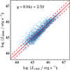 |
Fig. 1. Density distributions of luminosities at 1350 Å and 3000 Å for our sample. The solid and dashed red lines denote the best regression and its 1σ scatter, respectively. The best-fit result displayed in the panel was used to convert between the two luminosities. |
For the BH mass (MBH), we used the measurements from Wu & Shen (2022), based on broad C IVλ1549 and Mg IIλ2800 emission from the single-epoch spectra1. Priority was given to the Mg II because C IV-based BH masses can suffer from systematic biases (e.g., Ho et al. 2012; Mejía-Restrepo et al. 2016). Subsequently, the Eddington ratio (Lbol/LEdd) was computed based on the Eddington luminosity LEdd = 1.26 × 1038MBH/M⊙ erg s−1. Radio-loud AGNs are often associated with extreme variability, which makes them unsuitable for our analysis and thus need to be excluded (e.g., Vanden Berk et al. 2004; MacLeod et al. 2010). To identify radio-loud AGNs, we calculated the radio-to-optical flux ratio determined at 2500 Å (f2500) and 6 cm (f6 cm; Kellermann et al. 1989). We initially measured f2500 at the nearest continuum windows (2230, 3050, 3500, or 3800 Å) in the rest frame, depending on the redshift of the target, and subsequently extrapolated to 2500 Å by assuming a power-law continuum derived from the SDSS composite spectrum (fλ ∝ λ−1.56; Vanden Berk et al. 2001). We estimated f6 cm from the 20 cm flux density measurements of radio counterparts matched within 2″ from the FIRST survey (Lyke et al. 2020). For the flux conversion from 20 cm to 6 cm and k-correction, we assumed fν ∝ ν−0.5 (Kellermann et al. 1989; but see Ho & Ulvestad 2001). Objects with a radio loudness (R = f6 cm/f2500) greater than 10 (2954 objects) were classified as radio-loud objects and discarded for further analysis. The distributions of BH mass, bolometric luminosity, and Eddington ratio of the final sample of 91 897 sources are shown in Figure 2.
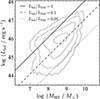 |
Fig. 2. Distributions of BH mass and bolometric luminosity for our sample. The solid, dashed, and dotted lines correspond to Eddington ratios of 1, 0.1, and 0.01, respectively. |
2.3. Continuum fluxes and uncertainties
To minimize the effect of the emission lines, including Fe II multiples, and starlight from the host galaxy, we estimated the continuum fluxes at 1367, 1479, 1746, 2230, 3050, 3500, and 3800 Å in the rest frame (Son et al. 2025). At each continuum wavelength, the flux was estimated using the mean flux value, and its uncertainty (σin) was calculated as  , where N is the number of spectral elements within a continuum window2 of 40 Å and σi is the uncertainty associated with each spectral element. However, the flux calibration of the SDSS spectra can introduce systematic uncertainty, which should be considered for accurate SF estimates (e.g., Margala et al. 2016; Son et al. 2025). While in principle this uncertainty can be estimated using multi-epoch spectra of standard stars, the standard stars are systematically brighter than our sample, which could possibly lead to an underestimate of the uncertainty.
Instead, we utilized the SF of the spectroscopic pairs in the AGN sample with short time intervals (Δt < 2 days in the observed frame), assuming that the AGN variability on such timescales is negligible. The SF of an observed pair was calculated as
 (1)
(1)
where Δt is the time lag between the observed pair, m is the observed magnitude at a given continuum wavelength, and σin is the initial uncertainty of magnitude in the single-epoch spectrum. We found that the average SF2 at Δt < 2 days (SF2days2) is mostly greater than 0 across all the continuum wavelengths, which indicates that the original uncertainties (σin) were significantly underestimated. Notably, the average SF2days2 depends on the continuum brightness and is well described by a double power-law model (Fig. 3). Therefore, we incorporate this excess, which depends on the flux density and continuum wavelengths, when estimating the structure function over longer timescales (Sect. 3.1). Specifically, the SF2 day2 was modeled using the form
![Mathematical equation: $$ \begin{aligned} \mathrm{{SF}}^2_{\rm {2days}}= A \left( \frac{f}{f_b} \right) ^ {-\alpha _1} \left\{ \frac{1}{2} \left[1 + \left( \frac{f}{f_b}\right)^{1 / \Delta } \right]\right\} ^{(\alpha _1 - \alpha _2) \Delta }, \end{aligned} $$](/articles/aa/full_html/2026/01/aa57713-25/aa57713-25-eq3.gif) (2)
(2)
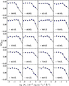 |
Fig. 3. Ensemble SF at Δt < 2 days (SF2days) plotted against continuum brightness across different wavelengths. The solid line represents the fitting results with a smooth double power-law model. |
where f is the continuum flux density, fb is the break flux density, A is the SF2days2 at the low-luminosity end, α1 is the power-law slope at fb ≫ f, α2 is the power-law slope when f ≫ fb, and Δ is the smoothness parameter. As α1 was found to be consistent with 0 across wavelengths, we fixed its value to 0 in the fit. As previous studies showed that the flux calibration is highly uncertain at the edges of the BOSS spectrum (Son et al. 2025), we restrict our analysis to spectra within the 3820–9150 Å range to minimize this effect.
3. Method and results
3.1. Analysis of spectral variability with ensemble SF
To analyze the AGN spectral variability, we utilized the ensemble SF of the spectral dataset. While SFs are typically calculated for individual objects, we grouped observed pairs of AGNs with similar physical properties instead (e.g., BH mass, bolometric luminosity, and Eddington ratio). We then computed the ensemble SF by averaging the individual SFs at each time lag. Therefore, the square of the ensemble SF was calculated as
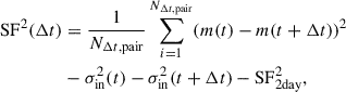 (3)
(3)
where NΔt, pair is the number of observed pairwise combinations at the given Δt across the AGN subsample, which shares similar AGN properties, and SF2day2 is estimated from the mean magnitude of the observed pairs. It is important to note that Δt was expressed in the rest frame for this calculation. We performed this analysis in each continuum window. The distributions of the number of observed pairs as a function of Δt across different continuum windows are shown in Figure 4. This indicates that a sufficient number of pairs exist up to Δt ≤ 1000 days. The extreme AGN variability can occur in a minority of AGNs, manifesting as changing-look AGNs, episodic flares, and tidal disruption events. These phenomena can substantially increase the variability amplitude and thus strongly influence the estimation of the ensemble SFs. Therefore, we applied the 3σ clipping method when averaging the SFs to minimize this effect.
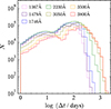 |
Fig. 4. Distribution of observed spectroscopic pairwise combinations at each Δt for our sample. Colors denote continuum wavelengths. |
3.2. Dependence of SF on AGN properties and wavelength
To explore how the SF varies with AGN properties and continuum wavelengths, we estimated the SFs for subsamples categorized by their AGN properties, such as BH mass, bolometric luminosity, and Eddington ratio. By accounting for the distributions of the physical parameters of the entire sample, we divided the sample into subgroups of five bins covering 1044.75 − 1046.30 erg s−1, 107.3 − 109.6 M⊙, and 10−2.2 − 100.3 for the AGN luminosity, BH mass, and Eddington ratio, respectively. On average, there are approximately 2500 pairwise combinations per bin, given wavelength, and Δt, ranging from 65 to about 19 000.
As illustrated in Figure 5, SFs are highly correlated with the bolometric luminosity and wavelengths. Notably, AGNs with higher luminosity or those at longer wavelengths tend to have lower SFs or longer variability timescales than their lower-luminosity or shorter-wavelength counterparts.
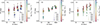 |
Fig. 5. Ensemble SFs for subgroups categorized according to bolometric luminosity (a), BH mass (b), and Eddington ratio (c). The size of the symbols denotes the continuum wavelength. |
The standard accretion disk model theoretically predicts that the thermal timescale is intrinsically tied to the orbital timescale. Previous observational studies also proposed that AGN variability timescales are governed by the thermal timescale (e.g., Collier & Peterson 2001; Kelly et al. 2009). This implies that the observed dependence of SFs on the AGN luminosity and wavelength can be interpreted through variations in the thermal timescale and the radial structure of the accretion disk. Accordingly, this model predicts that the variability timescale is strongly correlated with both AGN luminosity and wavelengths. Motivated by this, we quantified the dependence of the variability timescale on AGN luminosity and wavelength (τ ∝ Lαλβ), assuming that all AGNs share a universal ensemble SF when the time lag is normalized by the characteristic timescale (τ) (e.g., Tang et al. 2023; Son et al. 2025).
We assumed that SF ∝ a(Δt/τ)b, with τ scaling as τ ∝ Lαλβ, where a is the SF at Δt = τ and b is the power-law index for the entire sample. We then performed the fit using the ensemble SFs computed from subsamples divided by AGN luminosity and wavelength. In this calculation, we only included the ensemble SFs derived from more than 500 spectroscopic pairs to minimize a possible systematic error due to small sample sizes (Fig. 6). This analysis, which is based on the χ2 minimization, yields that τ ∝ L0.62 ± 0.07λ1.74 ± 0.23. At longer wavelengths (λ > 3050 Å), the continuum may be contaminated by the Balmer continuum from the BLR and by stellar light from the host galaxy. In particular, the effect of the Balmer continuum can be complex, as it may be less variable than the underlying continuum and its variability may be delayed due to the extended geometry of the BLR. To mitigate this, we repeated the experiment excluding the wavelengths greater than 3050 Å, which resulted in τ ∝ L0.68 ± 0.07λ1.12 ± 0.24. Specifically, the power-law index (β) for the wavelength changes dramatically from ∼1.74 to ∼1.12, which suggests a substantial contribution from either the Balmer continuum or the host light. Additionally, to mitigate the potential impact of outliers in the SFs, we applied a 3σ clipping during the fitting process. The fitting result remained unchanged within the uncertainties.
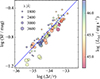 |
Fig. 6. Ensemble SFs with Δt normalized by the characteristic timescale (τ). We estimated τ assuming that all AGNs share a universal SF, with τ scaling as τ ∝ Lαλβ. |
For the Eddington ratio, similar trends were observed in the sense that AGNs with higher Eddington ratios tend to have smaller SFs or longer timescales, possibly due to their correlation with the AGN luminosity (Fig. 5a). With an assumption of the universal ensemble SF, we found τ ∝ (Lbol/LEdd)0.70 ± 0.08λ1.99 ± 0.24 when the fitting was done with the entire wavelength range up to 3800 Å. The fitting results also change significantly to τ ∝ (Lbol/LEdd)0.67 ± 0.08λ1.43 ± 0.31 when the wavelength over 3050 Å is excluded. However, intriguingly, the dependence of SFs on BH mass is not significant.
4. Discussion
4.1. Primary parameter that determines AGN variability
Based on the SF analysis for subgroups of the AGN sample, we found that the variability timescales strongly depend on both AGN luminosity and Eddington ratio. As noted in the previous section, the two parameters are closely linked to each other, which makes it difficult to identify the primary driver of AGN variability. To disentangle this degeneracy, we examined the effect of each parameter by fixing one parameter as a constant while varying the other. First, we selected a subset of AGNs with a narrow range of Eddington ratio (−1 ≤ log (Lbol/LEdd)≤ − 0.7) and recalculated the ensemble SFs for subsamples divided by AGN luminosity. To investigate the dependence of τ on AGN luminosity, we performed the same analysis under the assumption of a universal SF. This yielded a scaling relation of τ ∝ L0.95 ± 0.10λ4.15 ± 0.36. This analysis revealed that the variability timescale retains a significant dependence on AGN luminosity, which suggests that AGN luminosity plays an important role (Fig. 7). However, given the limited sample size3, the extracted scaling parameters should be interpreted with caution, as they may not reflect true physical relationships.
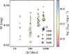 |
Fig. 7. Ensemble SFs of AGNs with a fixed Eddington ratio, grouped by bolometric luminosity. |
As a counterexample, we fixed the AGN luminosity within the range of 1045.8 − 1046.2 erg s−1, and assessed the ensemble SFs for subsamples categorized by Eddington ratio. Intriguingly, under these conditions, the dependence on the Eddington ratio vanished, as indicated by the relation τ ∝ (Lbol/LEdd)−0.01 ± 0.06 (Fig. 8). This result implies that the Eddington ratio has a minimal impact on the variability timescale when AGN luminosity is held nearly constant. Taken together, AGN luminosity is the main parameter that governs the variability timescales, rather than the Eddington ratio. We note, however, that the marginal correlation between the Eddington ratio and BH mass suggests that secondary effects resulting from this relationship warrant consideration. While this hypothesis could, in principle, be tested by additionally fixing the BH mass, the limited sample size precludes such an analysis within the scope of this study. Nevertheless, given that the BH mass appears to exert the least significant influence on the SF across the entire sample (Fig. 5), its impact is likely not dominant.
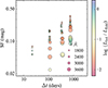 |
Fig. 8. Ensemble SFs of AGNs with a fixed bolometric luminosity, grouped by Eddington ratio. |
4.2. Physical interpretations
In theoretical studies based on the standard accretion disk framework, the thermal timescale scales as τth ∝ MBHR3/2, where R is the radial distance in the accretion disk. Additionally, the radial temperature profile of the disk follows  , where Ṁ represents the mass accretion rate. If the AGN luminosity is linearly correlated with Ṁ, the thermal timescale should be proportional to L0.5λ2 MacLeod et al. (2010), Tang et al. (2023), Son et al. (2025). Interestingly, this prediction is broadly consistent with our observational findings, which show that the variability timescale, inferred from the SFs, is primarily dependent on the AGN luminosity and wavelength.
Quantitatively, however, the best-fit power indices derived from our analysis (α = 0.62 ± 0.07 and β = 1.74 ± 0.23) exhibit marginal deviations from the theoretical prediction within a 2σ uncertainty. We note that the deviation in β dramatically increases when the wavelengths longer than 3050 Å, where substantial contamination from the Balmer continuum and stellar light is expected, are excluded from the fit (β = 1.12 ± 0.24). The fitted value of β falls below the theoretical prediction with a significance of ∼4σ. This result underscores the critical role of accurately accounting for host galaxy starlight and Balmer continuum contamination in studies of AGN variability.
Interestingly, the disagreement in β with the standard disk model has also been reported in previous observational studies (e.g., Son et al. 2025, but see also Tang et al. 2023). It is worthwhile noting that β is directly linked to the radial temperature profile under the assumption that the flux at a given wavelength primarily originates from the radius where the local temperature corresponds to that wavelength via Wien’s displacement law (λ ∝ 1/T). The significantly low value of β suggests that the radial temperature profile in the accretion disk may be steeper than predicted by the standard disk model (e.g., Son et al. 2025). This effect can result in a harder spectral energy distribution (SED) of the UV continuum, which is typically contrary to previous findings that report a softer-than-expected UV SED in AGNs (e.g., Zheng et al. 1997; Shang et al. 2005). The larger disk size, relative to predictions from the standard accretion disk model, can also be attributed to a shallower temperature profile (e.g., Sun et al. 2019). Conversely, an intrinsically harder UV continuum is required to explain the strength of broad emission lines in luminous AGNs (e.g., Lawrence 2012), which is consistent with a steeper temperature profile.
Alternatively, our results are consistent with predictions from the Corona-Heated Accretion-disk Reprocessing (CHAR) model, in which a steep temperature profile can be reproduced if the flux at a given wavelength is significantly contaminated by emission from neighboring radii (Sun et al. 2020). Within this framework, Zhou et al. (2024) demonstrate that the characteristic timescale depends on AGN luminosity and wavelength, with power-law indices of α = 0.65 and β = 1.19, which are in excellent agreement with our results. The results of Zhou et al. (2024) were derived from simulated light curves constructed using the AGN parameters of QSOs in Stripe 82, as adopted from Stone et al. (2022).
4.3. Comparison with previous studies
Mostly, AGN variability has been studied from a photometric dataset obtained with broadband filters (e.g., MacLeod et al. 2010; Sánchez-Sáez et al. 2018; Arévalo et al. 2023). Photometric data, however, can be severely affected by the emission from BLR, which can lead to systematic biases in characterizing the AGN variability. For example, based on the multi-epoch photometry of QSOs in Stripe 82, MacLeod et al. (2010) showed that τ exhibits moderate correlation with BH mass and wavelengths but little correlation with AGN luminosity. More recently, Arévalo et al. (2023) analyzed multi-epoch g-band photometry from the Zwicky Transient Facility (ZTF; Masci et al. 2019). Burke et al. (2021) analyzed broadband light curves from AGNs across a wide range of BH masses (104 M⊙ < MBH ≤ 1010 M⊙), collected from surveys like SDSS and various RM projects. Both studies discovered a correlation between τ and BH mass, contrary to the results in this study. Although the direct cause of this discrepancy with our findings remains unclear, it is worth noting that, unlike this study, Tang et al. (2023) estimated τ directly from the SFs or PSDs of multi-year broadband photometric light curves. Accurate measurements of τ are challenging, even when using light curves with baselines exceeding ten times the value of τ (Kozlowski 2017).
On the other hand, Tang et al. (2023) analyzed the approximately five-year multi-epoch broadband photometry of ∼5000 QSOs from the Asteroid Terrestrial-impact Last Alert System (ATLAS) survey using the same method in this study and found that τ is primarily governed by AGN luminosity and wavelength. While this result aligns with our finding, their reported value of β ∼ 2.4 is systematically larger than that obtained in this study. To examine the impact of broadband filters, we artificially generated the broadband photometric light curves using the spectroscopic datasets employed in this study. To mimic broadband conditions, we set the width of the continuum windows to 1000 Å. When we applied the same analysis method, we found α = 0.67 ± 0.06 and β = 2.13 ± 0.22, which agrees well with the results of Tang et al. (2023). More importantly, excluding continua with central wavelengths longer than 3050 Å yielded a similar trend (α = 0.68 ± 0.07 and β = 1.77 ± 0.28), with no significant change in the parameters derived from including the entire wavelength range. These findings demonstrate that, in broadband photometric data, contamination from strong emissions and the Balmer continuum originating from the BLR is non-negligible. Additionally, the range of AGN luminosity also differs among the observational studies (∼1046 − 47 erg s−1 for Tang et al. 2023 and ∼1044.8 − 46.2 erg s−1 for our study).
On the other hand, Son et al. (2025) utilized the multi-epoch spectroscopic dataset obtained through the SDSS RM project and analyzed the SFs of ∼800 QSOs, which, to our knowledge, was the first effort to specifically construct the SF for a large sample. Applying the same method in this study, they show that τ is mostly determined by AGN luminosity and wavelengths with α = 0.50 ± 0.03 and β = 1.42 ± 0.09. It is noteworthy that their results are consistent with ours at the ∼2σ level, despite the differences in the spectroscopic datasets: Son et al. (2025) employed an approximately seven-year time series of spectra for hundreds of QSOs, whereas this study used 2 million spectroscopic pairwise combinations for tens of thousands of QSOs. This confirms the reliability of our approach to explore AGN variability. Son et al. (2025) show that the fitting result for α and β is insensitive to the wavelengths of the continuum windows, revealing that the contribution from the Balmer continuum may not be crucial. However, on the contrary, the best-fitting value for β changes significantly with and without longer wavelengths above 3050 Å. This may be attributed to the fact that our sample comprises less luminous AGNs compared to Son et al. (2025), and hence the contribution from the host galaxy is more substantial in our sample.
To mitigate potential biases introduced by broadband photometric data and/or the limited range of AGN physical parameters resulting from a relatively small sample size, simultaneous monitoring with both photometric and spectroscopic datasets over a large sample is ideal. Such an approach will be enabled by the Time Domain Extragalactic Survey (Frohmaier et al. 2025) conducted with the 4 m Multi-Object Spectroscopic Telescope, in coordination with the Vera C. Rubin Observatory’s Legacy Survey of Space and Time (LSST; Ivezić et al. 2019).
5. Summary
We utilized multi-epoch spectroscopic data of ∼90 000 luminous AGNs from SDSS DR16 and examined the continuum ensemble SFs for subsamples categorized by various AGN properties, such as BH mass, AGN luminosity, and Eddington ratio. Based on this analysis, we reached the following conclusions:
-
Overall, the UV SFs are strongly dependent on wavelength, AGN luminosity, and Eddington ratio. However, they are weakly or barely correlated with the BH mass. To identify the primary parameter determining the SFs of AGNs, we re-examined the SFs by fixing either the AGN luminosity or the Eddington ratio. This revealed that the SFs are solely dependent on wavelength and AGN luminosity.
-
Under the assumption of a universal SF shared by all the AGNs in which the variability timescale (τ) is determined by wavelength (λ) and AGN luminosity (L), τ is found to scale with α = 0.62 ± 0.07 and β = 1.74 ± 0.23 following the equation τ ∝ Lαλβ. This finding aligns with the prediction (α = 0.5 and β = 2) from the standard disk model to within a 2σ level.
-
Excluding continua above 3050 Å allowed us to minimize the flux contribution from the host galaxy and Balmer continuum. We found β = 1.12 ± 0.24, which indicates a significant ∼4σ deviation from the standard disk model. This outcome may suggest that the temperature profile of the accretion disk is steeper than that predicted by the standard model.
-
The findings of this study significantly deviate from those of previous studies based on broadband photometric data. To robustly examine the dependence of SFs on AGN properties, particularly wavelength, it is essential to use spectroscopic datasets. This underscores the importance of spectroscopic monitoring of AGNs.
The BH masses were scaled to reflect the cosmological parameters adopted in this study.
We investigated the SF with a different width (e.g., 20 Å) and found that the main results in this paper remained unchanged with the uncertainties
We performed this experiment using approximately 0.15 − 0.39 million pairwise combinations depending on the continuum wavelength.
Acknowledgments
We are deeply grateful to the anonymous referee for insightful and constructive comments that have substantially enhanced the manuscript. LCH was supported by the National Science Foundation of China (12233001) and the China Manned Space Program (CMS-CSST-2025-A09). This work was supported by the National Research Foundation of Korea (NRF) grant funded by the Korean government (MSIT) (Nos. RS-2024-00347548 and RS-2025-16066624).
References
- Arévalo, P., Lira, P., Sánchez-Sáez, P., et al. 2023, MNRAS, 526, 6078 [CrossRef] [Google Scholar]
- Arévalo, P., Churazov, E., Lira, P., et al. 2024, A&A, 684, A133 [NASA ADS] [CrossRef] [EDP Sciences] [Google Scholar]
- Burke, C. J., Shen, Y., Blaes, O., et al. 2021, Science, 373, 789 [NASA ADS] [CrossRef] [Google Scholar]
- Burke, C. J., Shen, Y., Liu, X., et al. 2023, MNRAS, 518, 1880 [Google Scholar]
- Cardelli, J. A., Clayton, G. C., & Mathis, J. S. 1989, ApJ, 345, 245 [Google Scholar]
- Collier, S., & Peterson, B. M. 2001, ApJ, 555, 775 [NASA ADS] [CrossRef] [Google Scholar]
- Czerny, B., Schwarzenberg-Czerny, A., & Loska, Z. 1999, MNRAS, 303, 148 [NASA ADS] [CrossRef] [Google Scholar]
- Elvis, M., Wilkes, B. J., McDowell, J. C., et al. 1994, ApJS, 95, 1 [Google Scholar]
- Frohmaier, C., Vincenzi, M., Sullivan, M., et al. 2025, ApJ, 992, 158 [Google Scholar]
- Ho, L. C., & Ulvestad, J. S. 2001, ApJS, 133, 77 [NASA ADS] [CrossRef] [Google Scholar]
- Ho, L. C., Goldoni, P., Dong, X.-B., Greene, J. E., & Ponti, G. 2012, ApJ, 754, 11 [Google Scholar]
- Ivezić, Ž., Kahn, S. M., Tyson, J. A., et al. 2019, ApJ, 873, 111 [Google Scholar]
- Kasliwal, V. P., Vogeley, M. S., & Richards, G. T. 2015, MNRAS, 451, 4328 [CrossRef] [Google Scholar]
- Kaspi, S., Smith, P. S., Netzer, H., et al. 2000, ApJ, 533, 631 [Google Scholar]
- Kawaguchi, T., Mineshige, S., Umemura, M., & Turner, E. L. 1998, ApJ, 504, 671 [NASA ADS] [CrossRef] [Google Scholar]
- Kellermann, K. I., Sramek, R., Schmidt, M., Shaffer, D. B., & Green, R. 1989, AJ, 98, 1195 [Google Scholar]
- Kelly, B. C., Bechtold, J., & Siemiginowska, A. 2009, ApJ, 698, 895 [Google Scholar]
- Kim, M., Son, S., & Ho, L. C. 2024, A&A, 689, A27 [NASA ADS] [CrossRef] [EDP Sciences] [Google Scholar]
- Koshida, S., Minezaki, T., Yoshii, Y., et al. 2014, ApJ, 788, 159 [Google Scholar]
- Kozlowski, S. 2017, A&A, 597, A128 [NASA ADS] [CrossRef] [EDP Sciences] [Google Scholar]
- Kozlowski, S., Kochanek, C. S., Stern, D., et al. 2010a, ApJ, 716, 530 [CrossRef] [Google Scholar]
- Kozlowski, S., Kochanek, C. S., Udalski, A., et al. 2010b, ApJ, 708, 927 [CrossRef] [Google Scholar]
- Lawrence, A. 2012, MNRAS, 423, 451 [NASA ADS] [CrossRef] [Google Scholar]
- Li, Z., McGreer, I. D., Wu, X.-B., Fan, X., & Yang, Q. 2018, ApJ, 861, 6 [NASA ADS] [CrossRef] [Google Scholar]
- Lyke, B. W., Higley, A. N., McLane, J. N., et al. 2020, ApJS, 250, 8 [NASA ADS] [CrossRef] [Google Scholar]
- MacLeod, C. L., Ivezić, Ž., Kochanek, C. S., et al. 2010, ApJ, 721, 1014 [Google Scholar]
- Margala, D., Kirkby, D., Dawson, K., et al. 2016, ApJ, 831, 157 [NASA ADS] [CrossRef] [Google Scholar]
- Masci, F. J., Laher, R. R., Rusholme, B., et al. 2019, PASP, 131, 018003 [Google Scholar]
- Mejía-Restrepo, J. E., Trakhtenbrot, B., Lira, P., Netzer, H., & Capellupo, D. M. 2016, MNRAS, 460, 187 [CrossRef] [Google Scholar]
- Patel, P., Lira, P., Arévalo, P., et al. 2025, A&A, 695, A162 [NASA ADS] [CrossRef] [EDP Sciences] [Google Scholar]
- Peterson, B. M. 1993, PASP, 105, 247 [NASA ADS] [CrossRef] [Google Scholar]
- Petrecca, V., Papadakis, I. E., Paolillo, M., De Cicco, D., & Bauer, F. E. 2024, A&A, 686, A286 [NASA ADS] [CrossRef] [EDP Sciences] [Google Scholar]
- Planck Collaboration VI. 2020, A&A, 641, A6 [NASA ADS] [CrossRef] [EDP Sciences] [Google Scholar]
- Richards, G. T., Lacy, M., Storrie-Lombardi, L. J., et al. 2006, ApJS, 166, 470 [Google Scholar]
- Sánchez, P., Lira, P., Cartier, R., et al. 2017, ApJ, 849, 110 [CrossRef] [Google Scholar]
- Sánchez-Sáez, P., Lira, P., Mejía-Restrepo, J., et al. 2018, ApJ, 864, 87 [CrossRef] [Google Scholar]
- Schlafly, E. F., & Finkbeiner, D. P. 2011, ApJ, 737, 103 [Google Scholar]
- Shakura, N. I., & Sunyaev, R. A. 1973, A&A, 24, 337 [NASA ADS] [Google Scholar]
- Shang, Z., Brotherton, M. S., Green, R. F., et al. 2005, ApJ, 619, 41 [NASA ADS] [CrossRef] [Google Scholar]
- Shen, Y., Hall, P. B., Horne, K., et al. 2019, ApJS, 241, 34 [NASA ADS] [CrossRef] [Google Scholar]
- Shen, Y., Grier, C. J., Horne, K., et al. 2024, ApJS, 272, 26 [NASA ADS] [CrossRef] [Google Scholar]
- Smee, S. A., Gunn, J. E., Uomoto, A., et al. 2013, AJ, 146, 32 [Google Scholar]
- Son, S., Kim, M., & Ho, L. C. 2023, ApJ, 958, 135 [CrossRef] [Google Scholar]
- Son, S., Kim, M., & Ho, L. C. 2025, A&A, 695, A268 [NASA ADS] [CrossRef] [EDP Sciences] [Google Scholar]
- Stone, Z., Shen, Y., Burke, C. J., et al. 2022, MNRAS, 514, 164 [NASA ADS] [CrossRef] [Google Scholar]
- Suberlak, K. L., Ivezić, Ž., & MacLeod, C. 2021, ApJ, 907, 96 [NASA ADS] [CrossRef] [Google Scholar]
- Sun, M., Xue, Y., Trump, J. R., & Gu, W.-M. 2019, MNRAS, 482, 2788 [NASA ADS] [CrossRef] [Google Scholar]
- Sun, M., Xue, Y., Brandt, W. N., et al. 2020, ApJ, 891, 178 [CrossRef] [Google Scholar]
- Tang, J.-J., Wolf, C., & Tonry, J. 2023, Nat. Astron., 7, 473 [Google Scholar]
- Tonry, J. L., Denneau, L., Heinze, A. N., et al. 2018, PASP, 130, 064505 [Google Scholar]
- Ulrich, M.-H., Maraschi, L., & Urry, C. M. 1997, ARA&A, 35, 445 [NASA ADS] [CrossRef] [Google Scholar]
- Vanden Berk, D. E., Richards, G. T., Bauer, A., et al. 2001, AJ, 122, 549 [Google Scholar]
- Vanden Berk, D. E., Wilhite, B. C., Kron, R. G., et al. 2004, ApJ, 601, 692 [Google Scholar]
- Wu, Q., & Shen, Y. 2022, ApJS, 263, 42 [NASA ADS] [CrossRef] [Google Scholar]
- Zheng, W., Kriss, G. A., Telfer, R. C., Grimes, J. P., & Davidsen, A. F. 1997, ApJ, 475, 469 [NASA ADS] [CrossRef] [Google Scholar]
- Zhou, S., Sun, M., Cai, Z.-Y., et al. 2024, ApJ, 966, 8 [NASA ADS] [CrossRef] [Google Scholar]
All Figures
|
Fig. 1. Density distributions of luminosities at 1350 Å and 3000 Å for our sample. The solid and dashed red lines denote the best regression and its 1σ scatter, respectively. The best-fit result displayed in the panel was used to convert between the two luminosities. |
| In the text | |
|
Fig. 2. Distributions of BH mass and bolometric luminosity for our sample. The solid, dashed, and dotted lines correspond to Eddington ratios of 1, 0.1, and 0.01, respectively. |
| In the text | |
|
Fig. 3. Ensemble SF at Δt < 2 days (SF2days) plotted against continuum brightness across different wavelengths. The solid line represents the fitting results with a smooth double power-law model. |
| In the text | |
|
Fig. 4. Distribution of observed spectroscopic pairwise combinations at each Δt for our sample. Colors denote continuum wavelengths. |
| In the text | |
|
Fig. 5. Ensemble SFs for subgroups categorized according to bolometric luminosity (a), BH mass (b), and Eddington ratio (c). The size of the symbols denotes the continuum wavelength. |
| In the text | |
|
Fig. 6. Ensemble SFs with Δt normalized by the characteristic timescale (τ). We estimated τ assuming that all AGNs share a universal SF, with τ scaling as τ ∝ Lαλβ. |
| In the text | |
|
Fig. 7. Ensemble SFs of AGNs with a fixed Eddington ratio, grouped by bolometric luminosity. |
| In the text | |
|
Fig. 8. Ensemble SFs of AGNs with a fixed bolometric luminosity, grouped by Eddington ratio. |
| In the text | |
Current usage metrics show cumulative count of Article Views (full-text article views including HTML views, PDF and ePub downloads, according to the available data) and Abstracts Views on Vision4Press platform.
Data correspond to usage on the plateform after 2015. The current usage metrics is available 48-96 hours after online publication and is updated daily on week days.
Initial download of the metrics may take a while.