| Issue |
A&A
Volume 705, January 2026
|
|
|---|---|---|
| Article Number | A237 | |
| Number of page(s) | 8 | |
| Section | The Sun and the Heliosphere | |
| DOI | https://doi.org/10.1051/0004-6361/202558038 | |
| Published online | 21 January 2026 | |
Constraining the outer boundary condition for the Babcock-Leighton dynamo models
1
School of Space and Earth Sciences, Beihang University Beijing, People’s Republic of China
2
Key Laboratory of Space Environment Monitoring and Information Processing of MIIT Beijing, People’s Republic of China
3
Institute of Frontier and Interdisciplinary Science, Shandong University Shandong, People’s Republic of China
4
Institute of Space Sciences, Shandong University Shandong, People’s Republic of China
★ Corresponding author: This email address is being protected from spambots. You need JavaScript enabled to view it.
Received:
9
November
2025
Accepted:
8
December
2025
Abstract
Context. The evolution of the Sun’s large-scale surface magnetic field is well captured by surface flux transport models, which can therefore provide a natural constraint on the outer boundary condition (BC) of Babcock–Leighton (BL) dynamo models.
Aims. For the first time, we propose a zero radial diffusion BC for BL dynamo models, enabling their surface field evolution to align consistently with surface flux transport simulations.
Methods. We derived a zero radial diffusion BC from the magnetohydrodynamic induction equation and evaluated its effects in comparison with two alternatives: (i) a radial outer BC and (ii) a radial outer BC combined with strong near-surface radial pumping. The comparison was made both for the evolution of a single bipolar magnetic region and within a full BL dynamo model.
Results. The zero radial diffusion outer BC effectively suppresses radial diffusion across the surface, ensuring consistency between the evolution of the bipolar magnetic region in the BL dynamo and the surface flux transport model. With this outer BC, the full BL dynamo model successfully reproduces the fundamental properties of the solar cycle. In addition, the model naturally produces a surface magnetic field that is not purely radial, in closer agreement with solar observations.
Conclusions. The physically motivated zero radial diffusion BC paves the way for deeper insight into the solar and stellar cycles.
Key words: Sun: evolution / Sun: interior / Sun: magnetic fields / Sun: photosphere
© The Authors 2026
 Open Access article, published by EDP Sciences, under the terms of the Creative Commons Attribution License (https://creativecommons.org/licenses/by/4.0), which permits unrestricted use, distribution, and reproduction in any medium, provided the original work is properly cited.
This article is published in open access under the Subscribe to Open model. This email address is being protected from spambots. You need JavaScript enabled to view it. to support open access publication.
1. Introduction
Boundary conditions (BCs) are essential for solving partial differential equations within a bounded domain. They ensure problems are mathematically well posed and guide the selection of physically relevant solutions. In the context of solar and stellar dynamo equations, BCs play a crucial role in shaping the behavior of large-scale magnetic fields. For instance, Schubert & Zhang (2001) and Jiang & Wang (2006) suggested that imposing electrically conducting BCs at the core–shell interface facilitates the emergence of an oscillatory solution in α2 dynamo. Choudhuri (1984) showed that changing the outer BC for the azimuthal field (Bϕ) from Bϕ = 0 to ∂Bϕ/∂r = 0 affects the cycle period of the solar dynamo. Käpylä et al. (2010) found that for a given shear and rotation rate, the growth rate of the magnetic field is higher if a vertical field is adopted for the outer BC. Long-term observations and recent advances in our understanding of the solar surface magnetic field offer an opportunity to explore improvements to the outer BCs in solar dynamo models.
Over the past decade, direct observations have increasingly supported the Babcock–Leighton (BL) solar dynamo (Babcock 1961; Leighton 1969). The essence of this class of model is that the poloidal field is generated through the emergence of active regions (ARs) and their subsequent evolution across the solar surface. A key feature of the BL solar dynamo is that it is observationally guided (Cameron & Schüssler 2023). In the recently developed distributed-shear BL dynamo models, in which the toroidal field is generated in the bulk of the convection zone by the latitudinal shear (Zhang & Jiang 2022), the surface magnetic field plays a central role in modulating the cycle period and contributes to the time- and latitude-dependent regeneration of the toroidal field, thereby producing the butterfly diagram (Jiang & Zhang 2025). It is therefore natural to incorporate advances in our understanding of the solar surface magnetic field into the formulation of the outer BCs for the BL solar dynamo model.
Surface flux transport (SFT) models have been highly successful in advancing our understanding of the evolution of the solar surface magnetic field. The high-latitude radial component of the magnetic field (Br) is determined solely by processes that transport flux poleward across the surface from the activity belt at lower latitudes, behaving as passively advected corks. Leighton (1964) drew the analogy between the motion of magnetic flux elements due to the supergranulation over the surface and the motion of molecules in a gas, and wrote the transport equation as
 (1)
(1)
where the horizontal field (uh) corresponds to the differential rotation and the meridional flow at the solar surface, and ∇s2 is the Laplacian operator on the surface of a sphere. Knobloch & Rosner (1981) and DeVore et al. (1984) demonstrated that the turbulent diffusivity, ηs, appears as a result of the ensemble averaging procedure, thereby providing a physical basis for its use in modeling the large-scale field. Wang et al. (1989) successfully applied the model to examine the polar field evolution of cycle 21. Since then, this model has been extensively employed to explore the temporal evolution of the solar surface magnetic field. Comprehensive discussions of the development and applications of this modeling framework are provided in the reviews by Jiang et al. (2014) and Yeates et al. (2023). Most recently, Luo et al. (2025) demonstrated that the simulated spectra based on the model generally agree with observations for spherical harmonic degrees (l) ≲60.
When applying an SFT model to multiple solar cycles of varying strength, Schrijver et al. (2002) and Baumann et al. (2006) found that the polar fields systematically drift, as well as an absence of polar field reversals. They argued that this disagreement with observations reflects a conceptual deficiency in the original SFT model, and proposed that a radial diffusion term for Br should be included in Eq. (1) to remove the long-term memory of the surface flux. This raises the important question of whether radial magnetic flux indeed diffuses across the surface.
In the past decade, significant progress has been made in recognizing the cycle dependence of sunspot emergence. In particular, the cycle-averaged tilt angles are anticorrelated with the cycle strength (Dasi-Espuig et al. 2010; Jiao et al. 2021), and the cycle-averaged latitude is correlated with the cycle strength (Li et al. 2003; Solanki et al. 2008; Jiang et al. 2011). These dependences act as effective nonlinear mechanisms for modulating the polar field generation and, consequently, the solar cycle, and are referred to as tilt quenching and latitude quenching (Jiang 2020; Petrovay 2020; Karak 2020), respectively. By incorporating the cycle dependence of sunspot emergence into the source of an SFT model, Cameron et al. (2010) reproduced the polar field reversal over multiple solar cycles without the radial diffusion. Recently, Yeates et al. (2025) considered realistic AR configurations and successfully reproduced the evolution of polar fields across multiple solar cycles in line with observations without radial diffusion. Together, these studies suggest that additional radial diffusion across the surface is not required in the SFT process. Accordingly, for the BL-type dynamo models, the BCs should likewise be formulated to prevent the radial diffusion of the radial component of the magnetic field across the surface, ensuring consistency between the surface field evolution in BL dynamos and in SFT models.
Cameron et al. (2012) made the first attempts to use the evolution of the SFT model to constrain near-surface properties of the BL dynamo. They suggest that a strong enough near-surface downward pumping with a vertical outer BC is required to reproduce surface field evolution from BL dynamo models in agreement with that from SFT models. Applying the constraint to BL dynamo models has led to progress in understanding both the solar and stellar cycle (e.g., Jiang et al. 2013; Karak & Cameron 2016; Karak & Miesch 2017; Hazra et al. 2019; Zhang et al. 2022). Theoretically, near-surface radial pumping could arise from inhomogeneous turbulence or from a positive diffusivity gradient (Zeldovich 1957; Rädler 1968; Petrovay 1994). However, direct numerical simulations so far have primarily shown a downward transport of the large-scale magnetic field near the base of the convection zone (e.g., Tobias et al. 1998; Ossendrijver et al. 2002; Käpylä 2025). Moreover, the combination of strong near-surface pumping and a vertical BC results in the presence of only the radial magnetic field component above 0.95 R⊙ and in weak torsional oscillations (Zhong et al. 2024), both of which are inconsistent with observations. Furthermore, Whitbread et al. (2019) compared the evolution of surface magnetic fields simulated from 3D BL dynamo and SFT models. Their results suggest that the disconnect between emerged ARs and the toroidal fields in the convection zone would be required for the consistency between dynamo models and the surface magnetic fields. The typical 2D BL dynamo naturally satisfies the requirement of disconnection, enabling us to focus on the role of the outer BC.
The objective of this paper is to propose a new constraint on the outer BCs for the BL dynamo, motivated by SFT modeling, which requires that no radial diffusion of the radial magnetic field component occurs across the solar surface. This constraint provides a physically consistent link between the SFT and BL dynamo frameworks and offers a step toward more realistic modeling of the solar cycle.
In Sect. 2 we derive the zero radial diffusion BC for the BL dynamo. In Sect. 3 we present the numerical results by applying the zero radial diffusion BC to the distributed-shear BL dynamo model. Finally, Sect. 4 provides a summary of the results and a discussion of their implications.
2. Derivation of the zero radial diffusion BC for the BL dynamo
The evolution of large-scale magnetic fields in the Sun is governed by the magnetohydrodynamic induction equation, and the radial parts near the surface are expressed as
 (2)
(2)
where u is the velocity of flow field and η represents the turbulent diffusivity. We assumed that η varies only with radius and is independent of horizontal position. Specifically, the first term of Eq. (2) can be written as follows:
 (3)
(3)
where the subscripts r and h correspond to the radial and horizontal direction, respectively. The term ∇ ⋅ (uhBr) represents the horizontal advection for Br, and ∇ ⋅ (urBh) is related to the emergence of sunspot, the source term in the SFT model (Yeates & Muñoz-Jaramillo 2013; Jiang et al. 2014; Yeates et al. 2023).
The last term of Eq. (2) represents the diffusion process, and it can be expanded as follows:
 (4)
(4)
The first two terms on the right-hand side of Eq. (4) represent the horizontal diffusion, as shown in the 2D SFT model. Considering the axisymmetric assumption in our BL dynamo model, the last term involving the longitudinal gradient vanishes. The remaining third term represents an additional radial diffusion term (Schrijver et al. 2002; Baumann et al. 2006). This term is rewritten as
 (5)
(5)
where A is magnetic vector potential in the ϕ direction, and the axisymmetric large-scale magnetic field B(r, θ, t) is expressed in spherical coordinates as
![Mathematical equation: $$ \begin{aligned} {\boldsymbol{B}}(r,\theta ,t)=B_\phi (r,\theta ,t) \mathbf{e }_\phi + \nabla \times \left[A(r,\theta ,t)\mathbf{e }_{\phi }\right]. \end{aligned} $$](/articles/aa/full_html/2026/01/aa58038-25/aa58038-25-eq6.gif) (6)
(6)
In the BL-type model, if we adopt the assumption that there is no radial diffusion across the solar surface to be consistent with the original SFT models satisfying Eq. (1), Eq. (5) must vanish at the surface. This requirement corresponds to imposing the zero radial diffusion outer BC. DeVore et al. (1984) derived Eq. (1) from the ideal magnetohydrodynamic induction equation by decomposing the magnetic and velocity field into ensemble-averaged and fluctuating components, and by assuming that the large-scale magnetic field is predominantly radial so that horizontal field components are negligible (Bθ = 0 and Bϕ = 0). In contrast, in our derivation of the zero radial diffusion outer BC, the radial field component naturally decouples from the horizontal components when the term ∇ ⋅ (urBh) is neglected. This term is typically associated with flux emergence source in SFT models. As a consequence of this treatment, the latitudinal field component Bθ is permitted to exist at the solar surface, rather than being implicitly suppressed by the assumption of a purely radial field.
We note that Eq. (5) equal to zero is a general form that makes no diffusion across the surface for poloidal fields, and a reduction form has been applied in dynamo models. Cameron et al. (2012) incorporate radial pumping in addition to the radial outer BC in the BL dynamo model as follows,
 (7)
(7)
They obtain a surface evolution of the poloidal field that is consistent with that produced by SFT models. Radial pumping refers to the strong downward transport of magnetic flux near the solar surface, which tends to align the magnetic field predominantly in the radial direction. As a result, one obtains Bθ = 0 and  in the near-surface layer. The depth to which the relation Bθ = 0 holds depends on the penetration depth of the pumping. The near-surface pumping, along with the radial BC (Eq. (7)), makes the following equation approximately valid:
 (8)
(8)
Then, Eq. (8) at the surface is
![Mathematical equation: $$ \begin{aligned} {\left. \frac{\partial }{{\partial \theta }}\left[ \sin \theta \left( {B_\theta } + r \frac{{\partial {B_\theta }}}{{\partial r}}\right)\right] \right|_{r = {R_ \odot }}}=0. \end{aligned} $$](/articles/aa/full_html/2026/01/aa58038-25/aa58038-25-eq10.gif) (9)
(9)
Therefore, the radial BC combined with radial pumping can be regarded as a specific realization of the zero radial diffusion BC, obtained by setting both terms Bθ and  equal to zero.
The general formulation of the zero radial diffusion BC for the axisymmetric dynamo is
 (10)
(10)
Theoretically, the zero radial diffusion outer BC in an axisymmetric BL dynamo model could completely prevent magnetic diffusion across the surface, provided that the meridional flow does not subduct the poloidal field beneath the polar surface layers. Under this condition, the evolution of the surface radial field is expected to be consistent with that obtained from SFT models, after spatial averaging in the azimuthal direction. In the next section we verify this expectation through numerical simulations.
3. Numerical results
This section aims to evaluate whether the new BC can reliably suppress the radial diffusion of the radial component of the magnetic field across the surface, thereby ensuring consistency between the surface field evolution in BL dynamos and that in SFT models. We first briefly overview the 2D distributed-shear BL dynamo in Sect. 3.1. We next examine a simple case by comparing the time evolution of a single bipolar magnetic region (BMR) under different setups of the outer BC in Sect. 3.2. We further examine the effects of different numerical implementations of the BC in Sect. 3.3. The results of a full 2D distributed-shear BL dynamo model with the zero radial diffusion BC are presented in Sect. 3.4.
3.1. Overview of the 2D BL dynamo
The dynamo equations we solved to find the toroidal field (Bϕ) and the poloidal field represented by the magnetic vector potential (A) are
 (11)
(11)
![Mathematical equation: $$ \begin{aligned}&\frac{\partial B_\phi }{\partial t}+\frac{1}{r}\left[\frac{\partial (u_{r}rB_\phi )}{\partial r}+\frac{\partial (u_{\theta }B_\phi )}{\partial \theta }\right] \nonumber \\&\quad =\eta \left(\nabla ^{2}-\frac{1}{s^2}\right)B_\phi + s(\mathbf B_{p} \cdot \nabla \Omega )+\frac{1}{r}\frac{d\eta }{dr}\frac{\partial (rB_\phi )}{\partial r}, \end{aligned} $$](/articles/aa/full_html/2026/01/aa58038-25/aa58038-25-eq14.gif) (12)
(12)
where the profiles of the meridional flow up, angular velocity Ω, turbulent diffusivity η, and BL-type source term SBL will be specified in the following subsections and s = r sin θ. For the bottom boundary, we imposed a perfect conductor condition, corresponding to A = 0, ∂(rBϕ)/∂r = 0 at r = 0.65 R⊙ (Zhang & Jiang 2022).
For the outer BC, we considered three cases for comparison. Case 1 applies the newly proposed constraint for the vector potential A, Eq. (10), with Bϕ = 0 at r = R⊙. Case 2 follows Cameron et al. (2012), imposing a vertical magnetic field, i.e., ∂(rA)/∂r = 0, Bϕ = 0 at r = R⊙, along with strong near-surface radial pumping γ = 25 ms−1 as in their formulation. Case 3 adopts the same outer BC as Case 2 but omits the near-surface pumping, thereby permitting radial diffusion of the radial magnetic field across the surface. The potential-field outer BC is another commonly adopted form in dynamo modeling. However, since Cameron et al. (2012) demonstrated that it fails to reproduce results consistent with SFT modeling, we did not consider this case here.
The dynamo equations are numerically solved with the Crank-Nicolson scheme combined with an approximate factorization technique (van der Houwen & Sommeijer 2001) developed at Beihang University. The code is second-order accurate in both space and time. For the default case, the computational grid was set to 129 points in both the radial and latitudinal directions. The scheme for dealing with the outer BC will be further addressed in the following subsections.
3.2. Surface evolution of a single bipolar magnetic region in dynamo models
In this section we examine the evolution of a single BMR in the dynamo models under the three setups of the outer BC presented in the previous section. The initial field distributions of A and Bϕ follow Eqs. (9) and (10) of Cameron et al. (2012), representing an isolated BMR centered at approximately 15° latitude. The meridional flow (up) and turbulent diffusivity (η) profiles are the same as those in Sect. 2.1 of Cameron et al. (2012), ensuring direct comparability. The angular velocity (Ω) and radial pumping profiles are set as those in Zhang & Jiang (2022), which would not affect the results. The source term in the evolution equation of the poloidal field (SBL) is not considered, which allows us to assess whether the dynamo-based BMR evolution aligns with that from SFT models (cf. Fig. 2 of Cameron et al. 2012).
Within the framework of the SFT model (Fig. 2 of Cameron et al. 2012), the evolution of the isolated BMR involves a small fraction of the leading-polarity flux (modulated by the tilt angle) being transported to the southern pole, while the equivalent amount of following-polarity flux is advected to the northern pole. In the absence of additional flux emergence and owing to the balance between the poleward meridional flow and the equatorward diffusion, the resulting polar field can remain stable for millennia. Accordingly, the temporal evolution of the BMR in dynamo simulations is expected to produce this behavior, provided that radial diffusion across the surface is effectively suppressed.
Figures 1a–1c compare the temporal evolution of the BMR in dynamo models under the outer BCs of Cases 1–3. Figures 1a and 1b, corresponding to Cases 1 and 2, present similar behaviors, consistent with that from the SFT model described above. In contrast, Case 3 (Fig. 1c), which lacks near-surface pumping under the vertical BC, shows the two polarities transported to the same pole. The ensuing cancelation between the two polarities leads to a rapid decay of the polar field. This implies a substantial reduction in dynamo efficiency and results in dynamo behavior that differs markedly from Cases 1 and 2. The potential-field outer BC included in the dynamo produces a similar behavior to that of Case 3, as presented in Cameron et al. (2012).
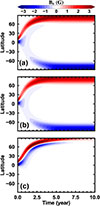 |
Fig. 1. Temporal evolution of an initial BMR on the solar surface obtained from dynamo simulations under the three outer BC settings: (a) zero radial diffusion outer BC (Case 1); (b) radial outer BC along with strong near-surface radial pumping (Case 2); and (c) radial boundary without near-surface radial pumping (Case 3). |
Figure 2 presents a quantitative comparison of the latitudinal distribution of Br at four time snapshots, i.e., t = 0.5 yr, 1.5 yr, 6.0 yr, and 10.0 yr. For all four times, Cases 1 and 2 exhibit nearly identical Br evolution, whereas Case 3 progressively diverges from their evolution with time. At t = 0.5 yr, magnetic flux remains concentrated in both polarities for all cases. At t = 1.5 yr, corresponding to the upper panel of Fig. 3 in Cameron et al. (2012), a small fraction of leading-polarity flux is transported to the southern hemisphere in Cases 1 and 2. At t = 6.0 yr, corresponding to the lower panel of Fig. 3 in Cameron et al. (2012), equal-magnitude polar fields have been established for Cases 1 and 2, while flux of both polarities is concentrated within one hemisphere, resulting in weaker total unsigned flux due to cancelation. At t = 10.0 yr, the polar fields remain nearly unchanged from t = 6.0 yr, with northern and southern polar fields of 3.07 G and −3.04 G, respectively. In contrast, the magnetic flux in Case 3 is almost completely canceled. These results clearly imply that BL dynamo models employing typical outer BCs, for example, vertical or potential-field BCs, tend to produce decaying solutions.
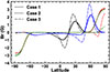 |
Fig. 2. Comparison of the latitudinal distribution of the surface radial field (Br) from dynamo simulations with three different outer BC settings. Shown are snapshots at t = 0.5 yr (black), t = 1.5 yr (blue), t = 6 yr (red), and t = 10 yr (green). Solid, dashed, and dot–dashed curves correspond to Cases 1, 2, and 3 of the outer BC, respectively. |
In summary, the newly proposed zero radial diffusion BC and the vertical BC with strong near-surface pumping both suppress radial diffusion in BL dynamo simulations, which leads to the same time evolution of a single BMR. However, residual diffusion remains unavoidable due to numerical effects, especially a second-order derivative is involved in the zero radial diffusion BC. Hence, we examine how numerical schemes for implementing the second-order derivative BC affect the evolution of an initial global poloidal field in the next subsection.
3.3. Influence of numerical schemes on the evolution of an initial global poloidal field
We used the magnetic field distribution at the end of the 10-year BMR evolution as the initial condition for the BL dynamo with the zero radial diffusion BC, which involves a second-order derivative. As in the previous subsection, no poloidal source term is included, and all other model parameters remain unchanged. In the absence of radial diffusion, the large-scale poloidal field is expected to remain stable for millennia because of the effect of the meridional flow. Near the equator, the poleward meridional flow inhibits cross-equatorial cancelation of the opposite radial flux, while in the polar regions, the balance between the poleward advection and the equatorward diffusion maintains the polar field (DeVore et al. 1984). To assess the influence of numerical schemes on suppressing radial diffusion, we applied the backward-difference scheme with varying orders of accuracy (second, third, and fourth) and two grid resolutions (129*129 and 259*259 in the radial and latitudinal directions). These tests enabled us to quantify how discretization errors and grid resolution affect the long-term stability of the poloidal field.
Table 1 summarizes the ten-year change rates of the polar field strength at nearly 89° latitude for various grid resolutions and discretization orders of the second-order derivative BC. For a resolution of 129 × 129 and second-order discretization accuracy, the radial magnetic field strength varies by approximately only 0.3% after ten years, so it is sufficient to conclude that the assumption of negligible radial diffusion is satisfied. Increasing the discretization order of the BC from second to third and fourth significantly reduces the change rate by nearly an order of magnitude. Higher spatial resolution further mitigates the numerical errors. At a 259 × 259 resolution, the change rate decreases nearly an order of magnitude to 0.061% with a second-order scheme, and to about 0.021% with a fourth-order scheme. Furthermore, the quantitative rates of change depend on the surface diffusivity and meridional flow speed. These results demonstrate that higher-order discretization and finer grid resolutions are effective in improving the numerical accuracy of the second-order derivative BC, thereby suppressing the radial diffusion.
Change rates of the polar field strength over 10 years for various grid resolutions and discretization accuracies of the second-order derivative BC.
Considering both accuracy and computational efficiency, we suggest that a 129 × 129 grid resolution combined with fourth-order discretization is an optimal numerical scheme for implementing the zero radial diffusion BC in dynamo simulations.
3.4. The distributed-shear BL dynamo with the zero radial diffusion BC
Zhang & Jiang (2022) developed the distributed-shear BL dynamo, which differs from the flux transport BL dynamo (Choudhuri et al. 1995; Dikpati & Charbonneau 1999; Chatterjee et al. 2004), as it does not rely on the subsurface meridional flow for flux transport (Jiang & Zhang 2025). The setup of the outer BC corresponds to Case 2 presented in Sect. 3.2, ensuring that the surface radial magnetic field evolves consistently with SFT models. Consequently, the poloidal field is dominated by large-scale components, primarily spherical harmonics l = 1, 3, and 5 (Luo et al. 2024). In the bulk of the convection zone, the poloidal field is primarily latitudinal, enabling the generation of the toroidal field by the latitudinal shear. Hence, it is termed the distributed-shear model. Unlike flux transport dynamos, the distributed-shear model relies critically on the surface magnetic field. The surface polar field, shaped by the surface flux source and transport process, dominates the cycle period. Moreover, the evolving surface field is a factor contributing to the time- and latitude-dependent regeneration of the toroidal field that gives rise to the characteristic of the solar butterfly diagram.
In Sect. 3.2 we demonstrate that applying the zero radial diffusion BC to the BL model effectively captures the evolution of a BMR. In this subsection we apply the same BC to the BL dynamo model of Zhang & Jiang (2022) to assess the resulting differences. Because we argue that the nonlinear mechanisms in the BL dynamo primarily arise from tilt-angle quenching (Dasi-Espuig et al. 2010; Jiao et al. 2021) and latitudinal quenching (Jiang 2020; Petrovay 2020; Karak 2020), we did not include the nonlinear algebraic quenching term in the source term SBL used by Zhang & Jiang (2022). Instead, we investigated the critical solution of a linear dynamo model. The parameter α0 was set to its critical value αc, which is determined as the value at which the growth rate of the dynamo solution approaches zero. We adopted ηCZ = 2.32 × 1011 cm2 s−1 and kept other parameters identical to those in the reference model of Zhang & Jiang (2022). The resulting critical value is αc = 2.35 ms−1.
Figure 3a shows the time-latitude diagram of the subsurface toroidal flux density calculated by integrating the toroidal field over the range of 0.7–1.0 R⊙ (see Eq. (8) of Zhang & Jiang 2022). Overall, the latitudinal migration pattern agrees with Fig. 4a of Zhang & Jiang (2022), which corresponds to the outer BC of Case 2. In each cycle, the antisymmetric toroidal field starts from about ±55° latitudes along with a residual branch from the previous cycle near the equator. As the cycle progresses, the toroidal field presents both a poleward migration with a duration of about 11 years and an equatorward migration lasting about 18 years, consistent with the extended solar cycle (Wilson et al. 1988; McIntosh et al. 2014). The two-branch pattern differs from the results of flux transport dynamo (FTD) models, which typically produce concentrated flux above ±70° latitudes due to strong radial shear in the polar tachocline. The poleward and equatorward branches of the toroidal field generated within the bulk of the convection zone in our model also provide a natural explanation for the observed torsional oscillation, driven by the Lorentz force associated with the cyclic magnetic field (Zhong et al. 2024).
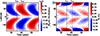 |
Fig. 3. Dynamo solution with the zero radial diffusion outer BC. (a) Temporal evolution of subsurface flux density of the toroidal field. (b) Temporal evolution of the surface radial fields. Cycle minimum (tmin) and cycle maximum (tmax) are indicated by the vertical dashed and dotted lines, respectively. |
A minor difference between our Fig. 3a and Fig. 4a of Zhang & Jiang (2022) is that the maximum mean flux density in this result is approximately a factor of two lower. Nevertheless, this amplitude remains within the reasonable range estimated for the solar toroidal flux generation rate by Cameron & Schüssler (2015). The discrepancy originates from the distinct magnetic transport mechanisms near the surface. In Zhang & Jiang (2022), strong downward pumping above 0.95 R⊙ rapidly transports the latitudinal field Bθ into deeper layers, where the latitudinal shear increases with depth (see Fig. 1d of Zhang & Jiang 2022), thereby enhancing toroidal-field generation. In contrast, under the Case 1 outer BC adopted here, Bθ is advected downward gradually by the turbulent diffusion η, resulting in the weaker toroidal-field amplification. Consequently, the peak toroidal field strength in our model is about 150 G, compared to about 450 G under the Case 2 BC adopted by Zhang & Jiang (2022). This value is also two orders of magnitude lower than the field strengths of buoyant magnetic loops in global convective-dynamo simulations (Nelson et al. 2013, 2014). We emphasize that our result represents an azimuthally averaged toroidal field and does not account for the intermittent concentration of magnetic flux tubes as a result of the turbulent convection.
Figure 3b shows the time-latitude diagram of the radial field Br at the solar surface. Overall, the result is consistent with Fig. 4b of Zhang & Jiang (2022) and with the observed magnetic butterfly diagram (Wang et al. 2025; Luo et al. 2025) in terms of the latitudinal migration pattern, the phase relation between the polar field and the activity cycle, and the polar field amplitude. Compared with observations, the absence of poleward surges in our model is likely due to the omission of ring doublets used to model individual AR emergence (Muñoz-Jaramillo et al. 2010).
The top panels of Fig. 4 illustrate the evolution of the poloidal field over a simulated solar cycle. The surface magnetic field is not strictly radial: near the poles, the radial component dominates, whereas at lower latitudes the latitudinal component becomes significant. This behavior contrasts with the Case 2 outer BC adopted by Zhang & Jiang (2022), where the surface field is enforced to be purely radial (see the top panel of their Fig. 6). Observations support that the polar field is nearly radial (Sun et al. 2021), and in the activity belts, the radial component typically dominates in regions of strong magnetic field, such as sunspots. Moreover, the field shown here is longitudinally averaged, corresponding to the magnetic butterfly diagram, where the mean radial field is only a few gauss. Meanwhile, a non-negligible large-scale latitudinal component Bθ is detected (Solanki et al. 2006). These observations explain the dominant latitudinal component at lower latitudes. Therefore, allowing a finite surface Bθ yields a more realistic representation of the large-scale solar surface field and can be regarded as an advantage of the current BC relative to Case 2.
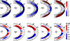 |
Fig. 4. Snapshots of the poloidal field (first row) and toroidal field (second row) over a dynamo cycle for the distributed-shear BL dynamo with the zero radial diffusion outer BC. Solid (dashed) contours in the top panels correspond to clockwise (counterclockwise) poloidal field lines. |
The low panels of Fig. 4 show the corresponding evolution of the toroidal field. The large-scale Bθ component generates a toroidal field within the bulk of the convection zone through the latitudinal differential rotation, consistent with the framework of the distributed-shear BL dynamo. For each cycle, the toroidal field originates near ±55° latitudes, and subsequently migrates both equatorward and poleward, driven by the latitudinal dependence of the latitudinal differential rotation. This behavior contrasts with that of FTD models. In addition to the strength of the poloidal field, turbulent diffusion plays a key role in the cyclic regeneration of the toroidal field by enabling flux cancelation between successive cycles for the rising phase and across the equator for the decline phase (Cameron & Schüssler 2016). These characteristics are generally consistent with those obtained using the Case 2 outer BC, except that the toroidal field here is slightly weaker, owing to the reduced strength of the corresponding poloidal field.
4. Discussion and conclusions
In this paper we have introduced a new outer BC, a zero radial diffusion BC, for the BL dynamo to ensure that the surface field evolution is consistent with observations. We have verified the effectiveness of this boundary treatment using both an individual BMR case and a full dynamo simulation. The BC is approximately equivalent to adopting a vertical-field condition combined with near-surface radial pumping, as proposed by Cameron et al. (2012), but offers two key advantages. First, the need to introduce radial pumping as an additional physical process is eliminated, in line with the spirit of Occam’s razor. Second, it naturally produces a surface magnetic field that is not purely radial, which is more consistent with solar observations. Our preliminary analysis further indicates that the new outer BC enables a more realistic reproduction of the surface distribution and temporal evolution of torsional oscillations, outperforming the Case 2 outer BC evaluated in Zhong et al. (2024).
With the surface field correctly maintained, the large-scale poloidal field dominates near the surface, leading to the generation of a toroidal field primarily in the bulk of the convection zone through latitudinal differential rotation, which is in the same scenario of distributed-shear BL dynamo (Zhang & Jiang 2022; Jiang & Zhang 2025) and the original BL dynamo (Babcock 1961; Leighton 1969). The realistically reproduced surface magnetic field also significantly enhances the dynamo efficiency by suppressing radial diffusion, in contrast to the widely used vertical-field outer BC and the potential-field matching BC. Our results highlight that the surface magnetic field produced by the emergence and evolution of ARs is a fundamental element of the BL dynamo loop. Yet, most previous BL dynamo models, such as the FTD models, do not incorporate realistic constraints on the surface boundary, resulting in surface field evolution inconsistent with observations and, consequently, altered dynamo behavior in the convection zone.
The outer BC matching a potential field outside the photosphere has been widely adopted in previous dynamo models. However, it is well recognized that the solar photosphere and corona exhibit non-potential magnetic structures (e.g., Gary et al. 1987; Seehafer 1990; Pevtsov et al. 1997). To quantify the non-potential and helical properties of the coronal magnetic field, Pipin (2025) incorporated the harmonic magnetic field as the outer BC, originally proposed by Bonanno (2016), into dynamo simulations. They argue that the non-potential and helical nature of the coronal magnetic field originates directly from the dynamo region (e.g., Käpylä et al. 2010; Warnecke et al. 2011). Similarly, weak horizontal surface fields are also permitted in the model of van Ballegooijen & Mackay (2007), who reproduced the observed spreading of AR magnetic flux across the solar surface by coupling magnetic field evolution in the convection zone with that in the corona. An alternative interpretation attributes these non-potential and helical properties to surface processes, including differential rotation, meridional flow, supergranular diffusion, and the emergence of twisted ARs (e.g., Yeates 2014; Yeates & Bhowmik 2022). The hemispheric pattern of filaments (van Ballegooijen et al. 1998; Yeates et al. 2007) has been successfully reproduced by coupling SFT models to coronal evolution models, in which the photospheric and coronal fields coevolve self-consistently. Our axisymmetric BL dynamo simulations reproduce the behavior of reduced 1D SFT models, where the large-scale radial field is spatially averaged in the azimuthal direction. We therefore anticipate that, when the zero radial-diffusion outer BC is implemented in a 3D kinematic distributed-shear BL dynamo, its surface magnetic evolution will be consistent with full SFT simulations. Consequently, the non-potential and helical coronal magnetic structures may also be reproduced in future extensions of our work.
In addition, we note that the zero radial diffusion BC we introduce involves a second-order radial derivative. The Cauchy problem for the second-order partial differential equations in Eqs. (11) and (12) is typically posed with Dirichlet, Neumann, or Robin BCs. There is no general existence theorem guaranteeing a well-posed solution when a second-derivative Neumann-type BC is imposed. Nevertheless, higher-order BCs, including second-order ones, have been widely used in practice when physically motivated. A common example arises in wave-equation problems, where such conditions have been successfully implemented (Engquist & Majda 1977; Bamberger et al. 1990; Poinsot & Lele 1992). These physically grounded boundary treatments robustly capture the essential dynamics of the system.
Acknowledgments
We thank the anonymous referee for the valuable comments and suggestions, which helped us to improve our manuscript. The research is supported by the National Natural Science Foundation of China (grant Nos. 12425305, 12350004, and 12173005).
References
- Babcock, H. W. 1961, ApJ, 133, 572 [Google Scholar]
- Bamberger, A., Joly, P., & Roberts, J. E. 1990, SIAM J. Numer. Anal., 27, 323 [Google Scholar]
- Baumann, I., Schmitt, D., & Schüssler, M. 2006, A&A, 446, 307 [NASA ADS] [CrossRef] [EDP Sciences] [Google Scholar]
- Bonanno, A. 2016, ApJ, 833, L22 [Google Scholar]
- Cameron, R., & Schüssler, M. 2015, Science, 347, 1333 [Google Scholar]
- Cameron, R. H., & Schüssler, M. 2016, A&A, 591, A46 [NASA ADS] [CrossRef] [EDP Sciences] [Google Scholar]
- Cameron, R. H., & Schüssler, M. 2023, Space Sci. Rev., 219, 60 [NASA ADS] [CrossRef] [Google Scholar]
- Cameron, R. H., Jiang, J., Schmitt, D., & Schüssler, M. 2010, ApJ, 719, 264 [NASA ADS] [CrossRef] [Google Scholar]
- Cameron, R. H., Schmitt, D., Jiang, J., & Işık, E. 2012, A&A, 542, A127 [NASA ADS] [CrossRef] [EDP Sciences] [Google Scholar]
- Chatterjee, P., Nandy, D., & Choudhuri, A. R. 2004, A&A, 427, 1019 [NASA ADS] [CrossRef] [EDP Sciences] [Google Scholar]
- Choudhuri, A. R. 1984, ApJ, 281, 846 [Google Scholar]
- Choudhuri, A. R., Schussler, M., & Dikpati, M. 1995, A&A, 303, L29 [NASA ADS] [Google Scholar]
- Dasi-Espuig, M., Solanki, S. K., Krivova, N. A., Cameron, R., & Peñuela, T. 2010, A&A, 518, A7 [NASA ADS] [CrossRef] [EDP Sciences] [Google Scholar]
- DeVore, C. R., Boris, J. P., & Sheeley, N. R., Jr. 1984, Sol. Phys., 92, 1 [NASA ADS] [CrossRef] [Google Scholar]
- Dikpati, M., & Charbonneau, P. 1999, ApJ, 518, 508 [NASA ADS] [CrossRef] [Google Scholar]
- Engquist, B., & Majda, A. 1977, Math. Comput., 31, 629 [Google Scholar]
- Gary, G. A., Moore, R. L., Hagyard, M. J., & Haisch, B. M. 1987, ApJ, 314, 782 [Google Scholar]
- Hazra, G., Jiang, J., Karak, B. B., & Kitchatinov, L. 2019, ApJ, 884, 35 [CrossRef] [Google Scholar]
- Jiang, J. 2020, ApJ, 900, 19 [Google Scholar]
- Jiang, J., & Wang, J.-X. 2006, Chinese J. Astron. Astrophys., 6, 227 [Google Scholar]
- Jiang, J., & Zhang, Z. 2025, A&A, 700, A210 [NASA ADS] [CrossRef] [EDP Sciences] [Google Scholar]
- Jiang, J., Cameron, R. H., Schmitt, D., & Schüssler, M. 2011, A&A, 528, A82 [NASA ADS] [CrossRef] [EDP Sciences] [Google Scholar]
- Jiang, J., Cameron, R. H., Schmitt, D., & Işık, E. 2013, A&A, 553, A128 [NASA ADS] [CrossRef] [EDP Sciences] [Google Scholar]
- Jiang, J., Hathaway, D. H., Cameron, R. H., et al. 2014, Space Sci. Rev., 186, 491 [Google Scholar]
- Jiao, Q., Jiang, J., & Wang, Z.-F. 2021, A&A, 653, A27 [NASA ADS] [CrossRef] [EDP Sciences] [Google Scholar]
- Käpylä, P. J. 2025, Liv. Rev. Sol. Phys., 22, 3 [Google Scholar]
- Käpylä, P. J., Korpi, M. J., & Brandenburg, A. 2010, A&A, 518, A22 [NASA ADS] [CrossRef] [EDP Sciences] [Google Scholar]
- Karak, B. B. 2020, ApJ, 901, L35 [NASA ADS] [CrossRef] [Google Scholar]
- Karak, B. B., & Cameron, R. 2016, ApJ, 832, 94 [NASA ADS] [CrossRef] [Google Scholar]
- Karak, B. B., & Miesch, M. 2017, ApJ, 847, 69 [NASA ADS] [CrossRef] [Google Scholar]
- Knobloch, E., & Rosner, R. 1981, ApJ, 247, 300 [Google Scholar]
- Leighton, R. B. 1964, ApJ, 140, 1547 [Google Scholar]
- Leighton, R. B. 1969, ApJ, 156, 1 [Google Scholar]
- Li, K. J., Wang, J. X., Zhan, L. S., et al. 2003, Sol. Phys., 215, 99 [NASA ADS] [CrossRef] [Google Scholar]
- Luo, Y., Jiang, J., & Wang, R. 2024, ApJ, 970, 76 [Google Scholar]
- Luo, Y., Jiang, J., & Wang, R. 2025, ApJ, 993, 27 [Google Scholar]
- McIntosh, S. W., Wang, X., Leamon, R. J., et al. 2014, ApJ, 792, 12 [NASA ADS] [CrossRef] [Google Scholar]
- Muñoz-Jaramillo, A., Nandy, D., Martens, P. C. H., & Yeates, A. R. 2010, ApJ, 720, L20 [CrossRef] [Google Scholar]
- Nelson, N. J., Brown, B. P., Brun, A. S., Miesch, M. S., & Toomre, J. 2013, ApJ, 762, 73 [Google Scholar]
- Nelson, N. J., Brown, B. P., Sacha Brun, A., Miesch, M. S., & Toomre, J. 2014, Sol. Phys., 289, 441 [NASA ADS] [CrossRef] [Google Scholar]
- Ossendrijver, M., Stix, M., Brandenburg, A., & Rüdiger, G. 2002, A&A, 394, 735 [NASA ADS] [CrossRef] [EDP Sciences] [Google Scholar]
- Petrovay, K. 1994, NATO Adv. Study Inst. (ASI) Ser. C, 433, 415 [Google Scholar]
- Petrovay, K. 2020, Liv. Rev. Sol. Phys., 17, 2 [Google Scholar]
- Pevtsov, A. A., Canfield, R. C., & McClymont, A. N. 1997, ApJ, 481, 973 [Google Scholar]
- Pipin, V. V. 2025, ArXiv e-prints [arXiv:2509.09985] [Google Scholar]
- Poinsot, T. J., & Lele, S. K. 1992, J. Comput. Phys., 101, 104 [Google Scholar]
- Rädler, K. H. 1968, Z. Naturforsch. A, 23, 1851 [Google Scholar]
- Schrijver, C. J., De Rosa, M. L., & Title, A. M. 2002, ApJ, 577, 1006 [Google Scholar]
- Schubert, G., & Zhang, K. 2001, ApJ, 557, 930 [Google Scholar]
- Seehafer, N. 1990, Sol. Phys., 125, 219 [NASA ADS] [CrossRef] [Google Scholar]
- Solanki, S. K., Inhester, B., & Schüssler, M. 2006, Rep. Progr. Phys., 69, 563 [CrossRef] [Google Scholar]
- Solanki, S. K., Wenzler, T., & Schmitt, D. 2008, A&A, 483, 623 [NASA ADS] [CrossRef] [EDP Sciences] [Google Scholar]
- Sun, X., Liu, Y., Milić, I., & Griñón-Marín, A. B. 2021, Res. Notes Am. Astron. Soc., 5, 134 [Google Scholar]
- Tobias, S. M., Brummell, N. H., Clune, T. L., & Toomre, J. 1998, ApJ, 502, L177 [NASA ADS] [CrossRef] [Google Scholar]
- van Ballegooijen, A. A., & Mackay, D. H. 2007, ApJ, 659, 1713 [NASA ADS] [CrossRef] [Google Scholar]
- van Ballegooijen, A. A., Cartledge, N. P., & Priest, E. R. 1998, ApJ, 501, 866 [Google Scholar]
- van der Houwen, P. J., & Sommeijer, B. P. 2001, J. Comput. Appl. Math., 128, 447 [NASA ADS] [CrossRef] [Google Scholar]
- Wang, Y. M., Nash, A. G., & Sheeley, N. R., Jr. 1989, ApJ, 347, 529 [Google Scholar]
- Wang, R., Jiang, J., & Luo, Y. 2025, ApJ, 987, 1 [Google Scholar]
- Warnecke, J., Brandenburg, A., & Mitra, D. 2011, A&A, 534, A11 [NASA ADS] [CrossRef] [EDP Sciences] [Google Scholar]
- Whitbread, T., Yeates, A. R., & Muñoz-Jaramillo, A. 2019, A&A, 627, A168 [NASA ADS] [CrossRef] [EDP Sciences] [Google Scholar]
- Wilson, P. R., Altrocki, R. C., Harvey, K. L., Martin, S. F., & Snodgrass, H. B. 1988, Nature, 333, 748 [Google Scholar]
- Yeates, A. R. 2014, Sol. Phys., 289, 631 [Google Scholar]
- Yeates, A. R., & Bhowmik, P. 2022, ApJ, 935, 13 [NASA ADS] [CrossRef] [Google Scholar]
- Yeates, A. R., & Muñoz-Jaramillo, A. 2013, MNRAS, 436, 3366 [NASA ADS] [CrossRef] [Google Scholar]
- Yeates, A. R., Mackay, D. H., & van Ballegooijen, A. A. 2007, Sol. Phys., 245, 87 [NASA ADS] [CrossRef] [Google Scholar]
- Yeates, A. R., Cheung, M. C. M., Jiang, J., Petrovay, K., & Wang, Y.-M. 2023, Space Sci. Rev., 219, 31 [CrossRef] [Google Scholar]
- Yeates, A. R., Bertello, L., Pevtsov, A. A., & Pevtsov, A. A. 2025, ApJ, 978, 147 [Google Scholar]
- Zeldovich, Y. B. 1957, Sov. Phys. JETP, 4, 460 [Google Scholar]
- Zhang, Z., & Jiang, J. 2022, ApJ, 930, 30 [NASA ADS] [CrossRef] [Google Scholar]
- Zhang, Z., Jiang, J., & Zhang, H. 2022, ApJ, 941, L3 [NASA ADS] [CrossRef] [Google Scholar]
- Zhong, C., Jiang, J., & Zhang, Z. 2024, ApJ, 969, 75 [Google Scholar]
All Tables
Change rates of the polar field strength over 10 years for various grid resolutions and discretization accuracies of the second-order derivative BC.
All Figures
|
Fig. 1. Temporal evolution of an initial BMR on the solar surface obtained from dynamo simulations under the three outer BC settings: (a) zero radial diffusion outer BC (Case 1); (b) radial outer BC along with strong near-surface radial pumping (Case 2); and (c) radial boundary without near-surface radial pumping (Case 3). |
| In the text | |
|
Fig. 2. Comparison of the latitudinal distribution of the surface radial field (Br) from dynamo simulations with three different outer BC settings. Shown are snapshots at t = 0.5 yr (black), t = 1.5 yr (blue), t = 6 yr (red), and t = 10 yr (green). Solid, dashed, and dot–dashed curves correspond to Cases 1, 2, and 3 of the outer BC, respectively. |
| In the text | |
|
Fig. 3. Dynamo solution with the zero radial diffusion outer BC. (a) Temporal evolution of subsurface flux density of the toroidal field. (b) Temporal evolution of the surface radial fields. Cycle minimum (tmin) and cycle maximum (tmax) are indicated by the vertical dashed and dotted lines, respectively. |
| In the text | |
|
Fig. 4. Snapshots of the poloidal field (first row) and toroidal field (second row) over a dynamo cycle for the distributed-shear BL dynamo with the zero radial diffusion outer BC. Solid (dashed) contours in the top panels correspond to clockwise (counterclockwise) poloidal field lines. |
| In the text | |
Current usage metrics show cumulative count of Article Views (full-text article views including HTML views, PDF and ePub downloads, according to the available data) and Abstracts Views on Vision4Press platform.
Data correspond to usage on the plateform after 2015. The current usage metrics is available 48-96 hours after online publication and is updated daily on week days.
Initial download of the metrics may take a while.