| Issue |
A&A
Volume 705, January 2026
|
|
|---|---|---|
| Article Number | C2 | |
| Number of page(s) | 9 | |
| Section | Stellar atmospheres | |
| DOI | https://doi.org/10.1051/0004-6361/202558767e | |
| Published online | 26 January 2026 | |
Enhancing the detection of low-energy M dwarf flares: Wavelet-based denoising of CHEOPS data (Corrigendum)
1
Departament de Física Quàntica i Astrofísica, Institut de Ciències del Cosmos (ICCUB), Universitat de Barcelona (IEEC-UB),
Martí i Franquès 1,
08028
Barcelona,
Spain
2
Institut d’Estudis Espacials de Catalunya (IEEC),
08860
Castelldefels (Barcelona),
Spain
3
Departament d’Enginyeria Electrònica i Biomèdica, Institut de Ciències del Cosmos (ICCUB), Universitat de Barcelona, IEEC-UB,
Martí i Franquès 1,
08028
Barcelona,
Spain
4
Institut de Ciències de l’Espai (ICE, CSIC), Campus UAB, c/de Can Magrans s/n,
08193
Bellaterra, Barcelona,
Spain
★ Corresponding author: This email address is being protected from spambots. You need JavaScript enabled to view it.
Key words: magnetic reconnection / instrumentation: detectors / stars: activity / stars: flare / stars: low-mass / errata, addenda
1 Error in flare energy calculation
In the original paper, flare energies were computed following the definition of Davenport (2016), that is, by multiplying the equivalent duration (ED), defined as the time integral of the flare profile normalised by the quiescent flux, by the stellar quiescent luminosity. In practice, this calculation relied on the implementation provided in the code of Bruno et al. (2024). As recently reported in the corrigendum of Bruno et al. (2025), the implementation of this calculation used an incorrect physical quantity: the ED was multiplied by the flare peak luminosity rather than the quiescent stellar luminosity, thereby introducing an additional multiplicative factor corresponding to the flare relative amplitude. Because our analysis adopts the same energy definition and relies on the same underlying formulation and code, this issue also affects the flare energies reported in our work. As a consequence, all flare energies quoted throughout our paper are systematically underestimated. This effect is more pronounced for the lowest-energy flares, for which the difference between peak and quiescent luminosity is largest in relative terms. Correcting this error results in a systematic upward rescaling of the flare-energy axis in all figures, tables, and derived quantities involving flare energy, as detailed in Section 2. Importantly, this correction does not affect:
the detection of flares in the CHEOPS light curves,
the flare recovery rate as a function of flare amplitude, Full Width Half Maximum (FWHM), spectral subtype, and wavelet function,
the relative comparison between flare samples extracted from original and wavelet-denoised light curves,
the identification and classification of simple versus complex flares,
the injection-recovery tests used to quantify detection completeness,
other measured flare parameters, such as duration, amplitude, impulse, and complexity,
the comparison between the AltaiPony-based detection and PEAKUTILS-based detection.
2 Summary of updated results
In Figure A.1, we present the updated injected-flare energy matrix corresponding to Figure 5 of the original paper, illustrating the upward rescaling of injected flare energies.
Figure A.2 presents the updated evolution of the confusion matrix metrics as a function of injected flare energy (updated Figure 9 of the original paper). This figure highlights the shift of the recovery turnovers towards higher energies for both the original and denoised simulated light curves, as well as the updated detection thresholds t1, t2, t3, and t4. These thresholds were recalculated to correspond to the same true positive rate (TPR) values of 10% and 90% as in the original analysis:
t1: TPR for denoised light curves exceeds 10% (1.8 × 1029 erg);
t2: TPR for original light curves exceeds 10% (5.6 × 1029 erg);
t3: TPR for denoised light curves reaches 90% (1.5 × 1030 erg);
t4: TPR for original light curves reaches 90% (7.1 × 1030 erg).
Figure A.3 shows the confusion matrices values obtained at these four thresholds (updated Figure 10 of the original paper).
The 215 flares detected in the original CHEOPS light curves now span energies from 1.3 × 1029 erg to 3.9 × 1032 erg. After wavelet denoising, the 291 detected flares also range from 1.3 × 1029 to 3.9 × 1032 erg. In the original light curves, the 101 individual components identified from the 48 complex flares range from 1.3 × 1029 to 2.9 × 1032 erg. In the denoised light curves, the 271 individual components recovered from 123 complex flares also span 1.3 × 1029 to 2.9 × 1032 erg. The increases in the total number of detected flares and in the number of recovered individual flare components remain unchanged at ~35% and ~65%, respectively. For complex flares, the number of recovered components increases by ~168%. The fraction of complex flares also remains unchanged at ~42%. However, due to the upward revision of the recovered energies, none of the detected events fall within the microflare energy regime. The conclusions of the original paper therefore remain valid for low-energy flares above this revised detection limit.
Figure A.4 presents the updated distributions and correlations between flare properties. Only panels involving flare energy differ from the original Figure 15. In the revised analysis, both the original and denoised flare energies show a clear inverse correlation with flare impulse, whereas this trend was absent for the denoised energies in the original version.
Figure A.5 shows the updated histograms for the detected flares per spectral subtype (updated Figure 17 of the original paper). The mean flare energies (second panel) have been updated, as well as the mean EDs (third panel), which were previously erroneously multiplied by the flare amplitude.
Figure A.6 shows the updated flare energy distribution histograms for the original and denoised samples. Similar to the original version, we find that the denoising mostly impacts the recovery of components of complex flares, indicating that denoising helps break down simple flares into their complex components.
Figure A.7 shows the observed correlations between flare parameters and stellar parameters. The only updated panel is the last one, which indicates a positive correlation between flare energy and distance (as in the original paper), reflecting an observational bias where only the most energetic flares are detected from distant sources.
Figure A.8 indicates the updated Flare Frequency Distributions (FFDs). The main difference is that complex flare components occur more frequently than simple flares across the entire energy range.
Table A.1 lists the updated alpha indices obtained from Figure A.8. We find that several subsamples reach the critical value of α > 2, above which smaller flares play a critical role in coronal heating, although caution is advised given the narrow energy range used for the fitting.
Figure A.9 shows the updated version of Figure 21, including the fits, log-likelihood ratios, and associated p-values comparing power-law and lognormal models for different subsamples. All subsamples are best described by a lognormal distribution. For the complex-flare subsample, the preference for the lognormal model now reaches statistical significance (p-value < 0.05). Overall, the statistical preference for a lognormal distribution is reinforced across all subsamples.
Figure A.7 shows the correlations between the denoised flares and the stellar parameters (updated Figure E.1). The only difference is the line corresponding to flare energy. No significant change results from the update, except that the correlation between flare energy and G-band magnitude is now slightly negative, whereas it was slightly positive in the original paper.
Figure A.11 shows the correlations between all flares and the stellar parameters (updated Figure E.2). The only difference is the line corresponding to flare energy. Here again, we note a slightly negative correlation between flare energy and G-band magnitude, indicating that low-energy flares are more easily recovered from bright stars, possibly due to an observational bias against dimmer targets.
3 Revised interpretation
The correction to the flare energy calculation results in a systematic upward rescaling of all reported flare energies. Consequently, the energy range of the detected events is revised, and the lowest-energy flares now lie above the microflare regime. Any interpretation in the original paper referring explicitly to microflares should therefore be disregarded.
Importantly, this correction does not affect the core results of this study. The detection of flares, the relative comparison between original and wavelet-denoised light curves, and the quantitative gains achieved through wavelet-based denoising remain unchanged. In particular, the stationary wavelet transform denoising continues to increase the number of recovered flares by ~35% and the number of recovered individual components of complex flares by ~65%, with a strong impact on the detection and decomposition of complex events.
All conclusions based on relative comparisons, such as the improved sensitivity to low-amplitude and short-duration flares, the enhanced breakdown of complex flare structures, and the consistency between AltaiPony- and PEAKUTILS-based analyses, remain valid. Likewise, the observed trends in flare frequency distributions, the dominance of complex flare components at lower energies, and the preference for a lognormal distribution are preserved after the correction.
Overall, while the absolute energy scale of the detected flares is revised, the main conclusion of the paper remains robust: wavelet-based denoising significantly enhances the ability of CHEOPS to detect and characterise low-energy stellar flares, extending the observable flare population towards weaker events relative to standard detection pipelines. This reinforces the value of advanced denoising techniques for exploiting high-cadence, high-precision photometric data in studies of stellar magnetic activity.
References
- Bruno, G., Pagano, I., Scandariato, G., et al. 2024, A&A, 686, A239 [NASA ADS] [CrossRef] [EDP Sciences] [Google Scholar]
- Bruno, G., Pagano, I., Scandariato, G., et al. 2025, A&A, 703, C4 [NASA ADS] [CrossRef] [EDP Sciences] [Google Scholar]
- Davenport, J. R. A. 2016, ApJ, 829, 23 [Google Scholar]
Appendix A Updated figures and tables
 |
Fig. A.1 Injected flare energy matrix as a function of the injected flare amplitude, FWHM, and spectral subtype. |
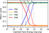 |
Fig. A.2 Evolution of confusion matrix metrics as a function of the injected flare energy. The TPR is shown in blue, the FPR in orange, the TNR in green, and the FNR in red. Metrics for the original light curves are represented by dashed lines, while those for the denoised light curves are shown as solid lines. The vertical dotted black lines indicate the four detection thresholds. |
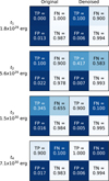 |
Fig. A.3 Confusion matrices from the flare injection and recovery process for the original (left) and denoised (right) light curves. The matrices are shown at the four detection thresholds, corresponding to TPR exceeding 10% (t1 and t2) and reaching 90% (t3 and t4), as defined in the original text. |
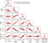 |
Fig. A.4 Corner plot of the different flare properties: relative amplitude, duration, measured energy, FWHM, impulse, and peak luminosity. The black data points represent individual flare components detected before denoising, while the red data points correspond to those detected after denoising. A linear fit is provided for reference in each distribution. The discrete bins for flare duration and FWHM arise from the 3-second observational cadence. |
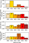 |
Fig. A.5 Flare statistics by spectral subtype for the stars in our sample. From top to bottom: Mean number of flares per star, updated mean flare energy, updated mean flare ED, and mean flare rate. The vertical bars represent the interquartile range (first to third quartiles), while the horizontal bars indicate the median values. In the M5V bin of the fourth panel, only one star is included, yielding identical values for the first quartile, median, and third quartile. |
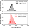 |
Fig. A.6 Histograms of the number of flares observed per energy bin. The grey-shaded histogram represents simple flares in denoised light curves, while the red-shaded histogram represents individual components of complex flares. The dashed black and red histograms show the same for the original light curves. |
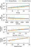 |
Fig. A.7 Correlations between flare parameters and stellar parameters. The blue and orange data points correspond to simple flares and individual components of complex flares, respectively. Each panel includes a linear fit for reference. |
 |
Fig. A.8 Flare frequency distributions for the flares recovered in our original (black) and denoised (red) samples. The FFDs are separated into simple flares (top left), individual components of complex flares (bottom left), flares on partially convective stars (top middle), flares on fully convective stars (bottom middle), and the full flare samples (top right). Bottom right: Comparison between the simple flares (blue) and individual complex flare components (orange) recovered from the denoised light curves (bottom right). The solid lines indicate linear fits to the double-logarithmic FFD, extrapolated into regimes not directly observed. |
Power-law indexes α obtained in Figure A.8
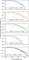 |
Fig. A.9 Complementary cumulative distribution functions for recovered flare energies in denoised light curves. Flares are separated into simple events (blue) and individual components of complex flares (orange), as well as flares from partially (green) and fully convective stars (purple). The full flare sample is displayed in black. Observed distributions, power-law fits, and log-normal fits are displayed with solid lines, dashed lines, and dotted lines, respectively. The vertical dashed grey lines indicate the 90% recovery energy (t3) and the start of the energy range used for the fitting. In each panel, the legend indicates the log-likelihood ratio R between the power-law and log-normal fits, along with its associated p-value. |
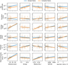 |
Fig. A.10 Correlations between denoised flare parameters and the host-star parameters, for simple flares (blue) and complex flare components (orange). Linear fits are shown for indication. |
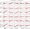 |
Fig. A.11 Correlations between flare parameters and host-star parameters, for the flares recovered from the original (black) and denoised (red) light curves. Linear fits are shown for indication. |
© The Authors 2026
 Open Access article, published by EDP Sciences, under the terms of the Creative Commons Attribution License (https://creativecommons.org/licenses/by/4.0), which permits unrestricted use, distribution, and reproduction in any medium, provided the original work is properly cited.
This article is published in open access under the Subscribe to Open model. This email address is being protected from spambots. You need JavaScript enabled to view it. to support open access publication.
All Tables
All Figures
|
Fig. A.1 Injected flare energy matrix as a function of the injected flare amplitude, FWHM, and spectral subtype. |
| In the text | |
|
Fig. A.2 Evolution of confusion matrix metrics as a function of the injected flare energy. The TPR is shown in blue, the FPR in orange, the TNR in green, and the FNR in red. Metrics for the original light curves are represented by dashed lines, while those for the denoised light curves are shown as solid lines. The vertical dotted black lines indicate the four detection thresholds. |
| In the text | |
|
Fig. A.3 Confusion matrices from the flare injection and recovery process for the original (left) and denoised (right) light curves. The matrices are shown at the four detection thresholds, corresponding to TPR exceeding 10% (t1 and t2) and reaching 90% (t3 and t4), as defined in the original text. |
| In the text | |
|
Fig. A.4 Corner plot of the different flare properties: relative amplitude, duration, measured energy, FWHM, impulse, and peak luminosity. The black data points represent individual flare components detected before denoising, while the red data points correspond to those detected after denoising. A linear fit is provided for reference in each distribution. The discrete bins for flare duration and FWHM arise from the 3-second observational cadence. |
| In the text | |
|
Fig. A.5 Flare statistics by spectral subtype for the stars in our sample. From top to bottom: Mean number of flares per star, updated mean flare energy, updated mean flare ED, and mean flare rate. The vertical bars represent the interquartile range (first to third quartiles), while the horizontal bars indicate the median values. In the M5V bin of the fourth panel, only one star is included, yielding identical values for the first quartile, median, and third quartile. |
| In the text | |
|
Fig. A.6 Histograms of the number of flares observed per energy bin. The grey-shaded histogram represents simple flares in denoised light curves, while the red-shaded histogram represents individual components of complex flares. The dashed black and red histograms show the same for the original light curves. |
| In the text | |
|
Fig. A.7 Correlations between flare parameters and stellar parameters. The blue and orange data points correspond to simple flares and individual components of complex flares, respectively. Each panel includes a linear fit for reference. |
| In the text | |
|
Fig. A.8 Flare frequency distributions for the flares recovered in our original (black) and denoised (red) samples. The FFDs are separated into simple flares (top left), individual components of complex flares (bottom left), flares on partially convective stars (top middle), flares on fully convective stars (bottom middle), and the full flare samples (top right). Bottom right: Comparison between the simple flares (blue) and individual complex flare components (orange) recovered from the denoised light curves (bottom right). The solid lines indicate linear fits to the double-logarithmic FFD, extrapolated into regimes not directly observed. |
| In the text | |
|
Fig. A.9 Complementary cumulative distribution functions for recovered flare energies in denoised light curves. Flares are separated into simple events (blue) and individual components of complex flares (orange), as well as flares from partially (green) and fully convective stars (purple). The full flare sample is displayed in black. Observed distributions, power-law fits, and log-normal fits are displayed with solid lines, dashed lines, and dotted lines, respectively. The vertical dashed grey lines indicate the 90% recovery energy (t3) and the start of the energy range used for the fitting. In each panel, the legend indicates the log-likelihood ratio R between the power-law and log-normal fits, along with its associated p-value. |
| In the text | |
|
Fig. A.10 Correlations between denoised flare parameters and the host-star parameters, for simple flares (blue) and complex flare components (orange). Linear fits are shown for indication. |
| In the text | |
|
Fig. A.11 Correlations between flare parameters and host-star parameters, for the flares recovered from the original (black) and denoised (red) light curves. Linear fits are shown for indication. |
| In the text | |
Current usage metrics show cumulative count of Article Views (full-text article views including HTML views, PDF and ePub downloads, according to the available data) and Abstracts Views on Vision4Press platform.
Data correspond to usage on the plateform after 2015. The current usage metrics is available 48-96 hours after online publication and is updated daily on week days.
Initial download of the metrics may take a while.