| Issue |
A&A
Volume 706, February 2026
|
|
|---|---|---|
| Article Number | A265 | |
| Number of page(s) | 11 | |
| Section | Extragalactic astronomy | |
| DOI | https://doi.org/10.1051/0004-6361/202554238 | |
| Published online | 13 February 2026 | |
The molecular and atomic hydrogen gas content of the Boötes Void galaxy CG 910
1
Key Laboratory of Radio Astronomy and Technology, Chinese Academy of Sciences Beijing 100101, People’s Republic of China
2
Physical Research Laboratory, Navrangpura Ahmedabad 380009, India
3
Indian Institute of Astrophysics, Koramangala Bangalore 560034, India
4
Max-Planck-Institut für Radioastronomie (MPIfR) Auf dem Hügel 69 53121 Bonn, Germany
5
New Cornerstone Science Laboratory, Department of Astronomy, Tsinghua University Beijing 100084, People’s Republic of China
★ Corresponding authors: This email address is being protected from spambots. You need JavaScript enabled to view it.
; This email address is being protected from spambots. You need JavaScript enabled to view it.
; This email address is being protected from spambots. You need JavaScript enabled to view it.
Received:
24
February
2025
Accepted:
27
October
2025
Abstract
Context. Void galaxies are located in the most under-dense environments of the Universe, where the number density of galaxies is extremely low. They are, hence, good targets for studying the secular evolution of galaxies and the slow buildup of stellar mass through star formation. Although the stellar properties of void galaxies have been studied, very little is known about their cold gas content, both molecular (H2) gas and atomic hydrogen (H I) gas.
Aims. We present CO (1–0) observations of the H2 gas disk in CG 910. CG 910 lies in the Boötes Void, one of the largest nearby voids, and is at relatively low redshifts (∼0.04–0.05). We selected CG 910 as it is a massive disk galaxy and early single-dish CO observations indicate that it has a high H2 gas mass. However, the H I content was not studied. Therefore, our aim was to map the cold disk, estimate the H I mass (and hence the total gas mass) in CG 910, and study the CO gas distribution along with the velocity field.
Methods. We used the Combined Array for Research in Millimetre Astronomy (CARMA) to study the CO(1–0) distribution and gas kinematics in CG 910. We also carried out atomic hydrogen observations of the galaxy using the Robert C. Byrd Green Bank Telescope (GBT). The stellar content of the galaxy and the star formation rate were derived using archival optical data.
Results. The CO(1–0) observations from CARMA reveal a molecular gas disk with a H2 mass of ∼12.0 ± 1.1 × 10⁹ M⊙ and a diameter of 7 kpc. The CO velocity field shows a regularly rotating disk with a flat rotation velocity of 256 kms−1 and no clear signatures of interaction or gas accretion. This is possibly the first CO (1–0) map of a void galaxy and, hence, important for understanding the molecular gas distribution and kinematics in void galaxies. The GBT observations reveal a H I disk with a H I mass of ∼3.1 ± 0.8 × 10⁹ M⊙, which is relatively low compared to the galaxy stellar mass (M★) of ∼21.5 × 10⁹ M⊙. The total gas mass fraction, (M(H2)+M(HI))/M★, and the atomic gas mass fraction, M(H I)/M★, for CG 910 are 0.70 and 0.14, respectively.
Conclusions. We conclude that CG 910 has a regularly rotating but massive molecular gas disk, which is more massive than the H I disk. The lower atomic gas mass fraction and star formation rate indicate a longer gas depletion timescale, confirming that, like most void galaxies, CG 910 is evolving more slowly than normal disk galaxies.
Key words: ISM: atoms / ISM: molecules / Galaxy: evolution / Galaxy: kinematics and dynamics / galaxies: star formation
© The Authors 2026
 Open Access article, published by EDP Sciences, under the terms of the Creative Commons Attribution License (https://creativecommons.org/licenses/by/4.0), which permits unrestricted use, distribution, and reproduction in any medium, provided the original work is properly cited.
This article is published in open access under the Subscribe to Open model. This email address is being protected from spambots. You need JavaScript enabled to view it. to support open access publication.
1. Introduction
Since the early redshift surveys of galaxies (Huchra et al. 1983), it has become clear that galaxies cluster along walls and filaments, leaving large empty regions called voids in between. Voids represent the most under-dense parts of the Universe and are close to spherical, with diameters of the order of 20–50 h−1 Mpc for voids with fewer luminous galaxies (van de Weygaert & Platen 2011). They are surrounded by walls, filaments, and clusters of galaxies, all of which form part of the cosmic web (Libeskind et al. 2018). Studies have shown that voids are not completely empty but are instead populated by a distribution of late-type, low-mass galaxies that are generally gas-rich and blue in colour (Kreckel et al. 2011; Beygu et al. 2017). They have lower stellar masses than galaxies in denser environments (Conrado et al. 2024), and a significant fraction are blue in colour, suggesting that they are mainly late-type, star-forming galaxies (Rojas et al. 2004). Only a small fraction show active galactic nucleus activity (Cruzen et al. 2002; Constantin et al. 2008), which is not surprising as most void galaxies do not have prominent bulges or spheroids and do not appear to have undergone much secular evolution. In fact, most void galaxies appear to be in a relatively ‘youthful’ state of evolution and lie in the blue part of the colour-magnitude plot for galaxies (Kreckel et al. 2012).
Since void galaxies reside in the most under-dense regions of the Universe, they are ideal systems for studying the slow, secular evolution of galaxies in low-density environments (Kreckel et al. 2011). They also represent one of the only ways to probe the interiors of voids and are hence important for various cosmological studies related to voids, such as the redshift space distortions in voids (Nadathur & Percival 2019) and the effect of dark energy on void evolution (Bos et al. 2012; Vielzeuf et al. 2021). Simulations suggest that the larger voids in the cosmic web are associated with the most massive clusters (mass > 1015 M⊙; Shim et al. 2021) and are connected with more filaments compared to the less massive clusters (mass < 1014 M⊙; Aragón-Calvo et al. 2010). The void galaxies in such simulations (e.g. TNG300) follow a slower evolutionary path compared to non-void galaxies, although they do undergo mass accretion via mergers at later times. They are also bluer and younger than galaxies in denser environments, which is similar to what is observed (Rodríguez-Medrano et al. 2024; Curtis et al. 2024). Observations also suggest that the larger voids contain more luminous, star-forming galaxies than the smaller voids. A good example is the nearby large and well-studied Boötes Void, which contains a significant population of star-forming, emission line galaxies, some of which also host active galactic nuclei (Weistrop et al. 1995; Cruzen et al. 1997; Pandey et al. 2021). In contrast, the smaller voids, such as the Local Void, contain mainly gas-rich, low-luminosity galaxies such as low-surface-brightness galaxies (Pustilnik et al. 2013) and ultra-diffuse galaxies (Román et al. 2019).
In the current understanding of structure formation, voids expand at a faster rate than the Hubble flow (Hoffman & Shaham 1982), resulting in the clustering of galaxies near the void walls (Ceccarelli et al. 2012). The void expansion thus results in smaller voids collapsing and hence merging to form larger voids (Sheth & van de Weygaert 2004; Russell 2014). This leads to the formation of a void substructure composed of smaller voids and filaments embedded in larger voids (van de Weygaert & Platen 2011), which are identified as ‘tendrils’ (Alpaslan et al. 2014). Void mergers also lead to the compression of the walls of the smaller voids and the formation of filaments within the voids. Such processes will push galaxies closer together and increase the rate of galaxy interactions and mergers, both of which lead to gas accretion and star formation. This suggests that the larger voids have the most luminous galaxies (Cruzen et al. 2002).
An important question related to void galaxies is what triggers their star formation and whether it is connected to the growth of void substructures (Das et al. 2015). On the scale of galaxy disks, star formation is often driven by interactions with close companions. For example, consider the galaxy pair CG 692-CG 693 in the Boötes Void (Weistrop et al. 1992) or triplets of galaxies in some nearby voids (Chengalur & Pustilnik 2013; Beygu et al. 2013). Star formation can also be triggered by gas accretion from filaments of the cosmic web (Egorova et al. 2019). The gas can flow from filaments within the voids onto the gas disks (Kleiner et al. 2017). The accreted gas cools the disk and increases the gas surface density, leading to the formation of local disk instabilities and star formation. Signatures of cold gas accretion in galaxies are extra-planar gas (plumes or filaments), warped gas disks, and lopsided gas distributions (Sancisi et al. 2008). These signatures can also be detected in the H I or CO velocity fields and represent gas cooling slowly onto the disks (Boomsma et al. 2008; Das et al. 2020). A similar phenomenon could be happening in the low-density environments of voids; cold gas accretion from the intergalactic medium along the filaments can drive disk star formation, resulting in the slow growth of galaxies. The neutral hydrogen (H I) surveys of void galaxies have detected some signatures of galaxy interactions, such as tidal tails, filaments, and extended H I disks (Szomoru et al. 1996).
Although void galaxies show signatures of star formation, surprisingly very little is known about their cold gas content. Some studies show that they have significant H I gas masses and extended H I disks (Kreckel et al. 2012), but there are only a few studies of the molecular gas content (Sage et al. 1997; Beygu et al. 2013; Das et al. 2015; Domínguez-Gómez et al. 2022). Studies of molecular gas disks and their gas kinematics can help one understand star formation processes in void galaxies. In this paper we report the results of CO(1–0) observations of the molecular gas distribution and the single-dish H I gas observations of the void galaxy CG 910, which lies in the Boötes Void. These observations are slightly dated, but we think these results should be presented since very little is known about the molecular gas disks of void galaxies. In fact, this work presents the first CO gas distribution and kinematics of a disk galaxy residing in a void. The paper is organised as follows. Section 2 describes the target galaxy in detail and the reasons for selecting it. In Sect. 3 we describe the observations and the data reduction of CO and H I emission. In Sect. 4 we present the results, including gas content and morphology. We further discuss the significance of this study of the gas content in CG 910 in Section 5, and finally conclude in Section 6.
2. The target galaxy CG 910
We selected CG 910 as it is one of the few void galaxies that have been detected in CO emission and has a high CO flux density (Sage et al. 1997). The galaxy lies within the Boötes Void, a large nearby void (size of ∼60 Mpc) with a relatively large population of bright galaxies (Cruzen et al. 2002). Figure 1 shows the archival Sloan Digital Sky Survey (SDSS; York et al. 2000) r-band emission map of CG 910. It has an optical disk of diameter ∼10″, or ∼9.5 kpc, a prominent bulge, and ongoing nuclear star formation, which is evident from its nuclear SDSS spectrum and centrally concentrated Hα emission. The latter is evident in the SDSS-MANGA (Mapping Nearby Galaxies at APO) map of the galaxy. Using the SDSS Hα flux value of 1.044 × 10⁻¹⁴ ergs cm−2 s−1, distance as 188 Mpc and the star formation rate (SFR) relation from Kennicutt et al. (1994), we obtain SFR = 0.33 M⊙ yr−1. Hence, CG 910 has a fairly moderate SFR, but it is relatively strong compared to the SFR of other void galaxies (Domínguez-Gómez et al. 2022).
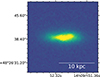 |
Fig. 1. SDSS r-band image of CG 910. |
The galaxy shows radio continuum emission at 1.4 GHz in the NRAO VLA Sky Survey (NVSS) image with a flux density of ∼4.7 mJy/beam and also in the Faint Images of the Radio Sky at Twenty Centimeters (FIRST) image, where it appears as a compact core that is associated with the nucleus. There is no prior H I observation of CG 910, but the CO(1–0) line has been observed using the Institute for Radio Astronomy in the Millimetre Range (IRAM) 30 m telescope (Sage et al. 1997). Table 1 summarises the properties of CG 910. The stellar mass is the best-fit value of the galaxy derived by fitting stellar evolution models to the SDSS photometry using the Portsmouth method and assuming the Kroupa initial mass function (IMF). The galaxy has very few neighbours; its nearest neighbour (WISEA J141018.54+482510) is at a projected distance of 229.4 kpc and also at a redshift similar to that of CG 910 (which we determined using the NED Cone search tool). The properties of the closest neighbour are also summarised in Table 1. Thus, CG 910 appears to be a spiral galaxy with a prominent bulge and a relatively high molecular gas content, showing signatures of ongoing star formation.
Properties of the CG 910 void galaxy.
3. Observations and data reduction
3.1. 12CO (1-0) CARMA data
The 12CO (1-0) observations of CG 910 were made using the Combined Array for Research in Millimetre Astronomy (CARMA) array of 15 antennas in the D-band configuration, with only the nine 6 m Berkeley-Illinois-Maryland Association (BIMA) dishes and six 15 m Owens Valley Radio Observatory (OVRO) dishes. The actual bandwidth of the correlator window containing the CO line is 470 MHz with 15 channels, with a velocity resolution of 81 km s−1. The observations were carried out for a duration of 3.5 hours in June 2014 with an integration time of 2 hours on CG 910. The visibility calibrator is 1419+543; the bandpass calibrator and the flux calibrator were 3C84 and Mars, respectively. The data reduction package MIRIAD (Sault et al. 1995) was used to reduce the interferometric data. A robust weighting was used with the robust parameter of 0.5. The angular resolution of the beam is 3.1″ × 2.4″ with position angle ∼90°. The RMS noise in the channel maps is 4.4 mJy/beam.
3.2. HI Green Bank Telescope data
To study the atomic content of the galaxy, we first observed the H I of CG 910 using the Effelsberg Radio telescope in June and July 2015. We applied a running median-filter-based flagging algorithm with subsequent interpolation to mitigate narrow-band radio frequency interference. The flux density calibration was done following (Winkel et al. 2012). The galaxy systemic velocity is in the radio convention and is v = 12 583 km s−1 (where v(radio) = (λ − λ0)/λ and v(optical) = (λ − λ0)/λ0). However, there is strong radio interference (from a nearby radar at 1360 MHz) in the band, which overlaps with the potential H I emission from the galaxy. This emission at the high-frequency side of this radio frequency interference could be H I emission from CG 910, and so further observations were needed to confirm the presence of H I.
We further conducted H I observations of CG 910 using the 100 m Robert C. Byrd Green Bank Telescope (GBT) located in West Virginia. The observations were done in February 2016 and were carried out for a duration of 10 hours spread over two days. The back-end instrument, VEstalise GB Astronomical Spectrometer (VEGAS) in the L band in the frequency range of 1.15–1.73 GHz was used for the spectroscopic observations. The bandwidth is 1500 MHz (effective bandwidth is 1265 MHz) with a channel resolution of 1465 kHz. The position-switching mode was used. The GBTIDL software (Marganian et al. 2013) was used for the calibration and processing of H I data. The noise achieved in RMS after the calibration is 0.48 mJy. Table 2 shows the details of observation and data reduction.
Observation details.
4. Results
4.1. 12CO emission
The 12CO (1-0) line emission from galaxies traces the molecular gas component and is usually more centrally concentrated than the H I gas distribution. To study the intensity distribution in the different channels, we made channel maps in the velocity range from 12 746.3 km s−1 to 12 339.9 km s−1 as shown in Fig. 2. The channel maps are made using the standard routine, ‘KNTR’ in the Astronomical Image Processing System (AIPS) software, which creates a contour plot from the data. Emission from the galaxy is detected in four consecutive channels (from panels 2–5). In each of these four channels, we observe the signature of a possible extended emission located in the south-west corner of the galaxy. The probable existence of this extended emission is based on a 1-sigma detection. However, it can also be observed with 2-sigma confidence in panels 2 and 4.
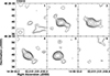 |
Fig. 2. Channel maps for CG 910 based on 12CO (1-0) data. The velocity in the first panel is 12 746.3 km s−1, with a velocity resolution of −81.2 km s−1. Contour levels are set at 6.5 × (1, 1.4, 2, 2.8, 4, 5.6, 8, 11.2, 16, 22.4, 32, 44.8, 64) mJy/beam, where 6.5 mJy/beam represents the RMS noise at a line-free channel of the data cube. |
Figure 3 represents the 12CO moment maps. These moment maps are made using the standard routine, ‘MOMNT’ of AIPS, following the procedure described in Biswas et al. (2022), i.e. by selecting the consecutive channels where at least 3σ emission is found in the cube, where σ is the RMS noise of a line-free channel. This includes four channels whose velocities range from 12 746.3 km s−1 to 12 339.9 km s−1. We then measured the RMS noise from a line-free channel, 4.961 mJy/beam and used a cutoff of 1.4 times the RMS noise to make the moment maps. Further details of this procedure are described in Biswas et al. (2022). Figure 3a represents the integrated 12CO emission, i.e. the moment zero map (the red contours), plotted over the SDSS r-band image. The molecular gas disk, traced by 12CO emission, is ∼14″ in diameter, or 13 kpc. In the moment zero map, we see a signature of the extended 12CO emission in the south-west direction of the galaxy, detected with a 2-sigma confidence level. Figure 3b shows the velocity field or the moment one map of the galaxy. The gradient of the velocity field, which is a result of the galaxy’s rotation, is clearly seen in this figure. The velocity of the molecular disk ranges from ∼12 400 km s−1 to ∼12 700 km s−1. Figure 3c shows the velocity dispersion map or the moment two map of the galaxy. The velocity dispersion map shows that the centre of the molecular disk has a high-velocity dispersion of ∼90 km s−1 and gradually decreases towards the end of the molecular disk to a value ∼10 km s−1.
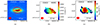 |
Fig. 3. 12CO (1-0) moment maps of CG 910. In panel (a), the red contours, which represent the 12CO emission, are plotted over the SDSS r-band image. The contours are set at (1, 2, 4, 8...) mJy/beam-km/s sigma levels. In panel (b), contours are set at 20 km s−1 intervals. The red patch at the bottom-left corner of each image represents the beam of the 12CO map. |
4.2. CO line profile and molecular hydrogen gas mass
We further examined the 12CO line profile obtained from the CARMA data. To extract the 12CO spectra from the CARMA data cube, we first masked the data cube using the moment zero map of 12CO. To do that, we first drew a region around the moment zero map where the emission is seen and blank all the other regions using the standard task, ‘BLANK’ of AIPS. This blanked moment zero map was further used to mask the three-dimensional data cube so that in each channel of the data cube, only the region defined by the moment zero map has data and all the other regions are blanked. This was also done using BLANK. This masked cube was then used to extract the spectra using the task ‘ISPEC’ of AIPS (Biswas et al. 2022). The obtained spectrum is shown in Fig. 4. The figure also shows a comparison of the 12CO spectra obtained in the IRAM 30-metre single-dish observation. The single-dish 12CO spectrum has been kindly provided by Sage et al. (1997) through private communication. The original spectrum from Sage et al. (1997) represents the brightness temperature in units of Kelvin. We converted this brightness temperature (K) to flux density (Jy), considering the IRAM beam following the procedure outlined in Alatalo et al. (2011).
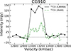 |
Fig. 4. 12CO spectra extracted from CARMA observations (in black) and IRAM 30 m single-dish observations (in green; Sage et al. 1997). |
From Fig. 4, we find that the 12CO spectra from CARMA differ from IRAM significantly, mostly in terms of amplitude. However, this large discrepancy in spectra between CARMA and IRAM is not new. Alatalo et al. (2013) found that for ∼50% of their total sample, which includes 30 galaxies, CARMA fluxes are higher than those obtained from IRAM. Alatalo et al. (2013) clearly note that if the angular extent of the molecular gas disk – mainly the diffuse structures with a low signal-to-noise ratio, such as rings, spiral arms, and tidal features – extends beyond a radius of 12″, it can be missed by the beam of the 30-metre dish of IRAM. In the case of CG910, the radius of the molecular disk is found to be 7.1″. This radius is found from the semi-major axis of an ellipse fitted to the one-sigma contour of the moment zero map from CARMA 12CO observation. However, we have also found extended emission associated with the galaxy through the position–velocity (PV) diagram extracted at different position angles with a diameter of ∼14″ (see Fig. 5; details about the PV diagram are provided in the later sections of the paper). This extended emission anticipated from the PV diagram is the most probable reason behind the discrepancy in the spectra between the CARMA and IRAM observations. It is to be noted that similar phenomena have been observed in the study of Alatalo et al. (2013) also, for example, for NGC 1222 and NGC 4119, the emission in PV diagram extends beyond a radius of 12″ but the radius roughly estimated from the moment zero maps, are in between ∼7″ and 9″. Both of them have significantly higher flux in their CARMA spectra than in the IRAM spectra.
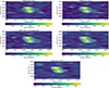 |
Fig. 5. PV diagram along different slices of the galaxy. The white contours are drawn at RMS × (1, 1.4, 2, 2.8, 4, 5.6, 8, ...) levels; the RMS is measured from a line-free channel of the 12CO data cube. |
From the CO spectrum obtained from the CARMA observation, we further measured the molecular gas mass of the galaxy. To do that, we first found the line-flux of the 12CO line. For that, we first took the RMS noise from the line-free channel of the 12CO spectrum. This RMS noise was then subtracted from the whole spectrum. This was done to remove any additional continuum emission that can remain after the continuum subtraction of the data cube. Then, we drew a line at 3 times the RMS above the spectra to find out the channel range of the integration to obtain the 12CO line-flux. The obtained line flux was then used to determine the 12CO luminosity using the following equation (Solomon & Vanden Bout 2005):
![Mathematical equation: $$ \begin{aligned} L_{CO} [K\,km\,s^{-1}\,pc^{2}] = 3.25\times 10^{7}\,S_{CO} \Delta V D_{L}^2 (\nu _{\rm obs})^{-2} (1+z)^{-3}, \end{aligned} $$](/articles/aa/full_html/2026/02/aa54238-25/aa54238-25-eq1.gif) (1)
(1)
where ΔV is the velocity resolution of the 12CO data in kms−1, SΔV is the integrated line-flux in Jy kms−1, νobs is the observed frequency in GHz (which is 110.44 GHz), DL is the luminosity distance and z is redshift of the galaxy. From the obtained 12CO luminosity, we calculated the molecular hydrogen gas mass of the galaxy using the following equation (Bolatto et al. 2013; Domínguez-Gómez et al. 2022): M(H2) = αCO LCO where, αCO is the CO-to-H2 conversion factor taken as 3.2 M⊙ (K km s−1 pc2)−1 (Bolatto et al. 2013; Domínguez-Gómez et al. 2022). Finally, the molecular gas mass (Mmol) of the galaxy was obtained with the correction for helium contribution by taking αCO = 4.6. The integrated 12CO line-flux, derived 12CO mass, and molecular gas mass are listed in Table 3. The measured 12CO flux and the molecular hydrogen gas mass are also compared with the IRAM 12CO spectra from Sage et al. (1997). It is to be noted that the 12CO line-flux and the H2 mass provided in Sage et al. (1997) are similar to what we note in Table 3 despite us using a different distance. However, if we use the distance taken by Sage et al. (1997) in our study, the 12CO line-flux and the H2 mass are still similar to what Sage et al. (1997) found in our study.
Line fluxes and masses of the molecular and atomic hydrogen gas.
4.3. Position–velocity diagram
Since we found some indication of extended emission in the channel maps (Fig. 2) and from the moment zero map (Fig. 3a), we further investigated the PV diagram of the galaxy. To do so, the position angle was first calculated using the following procedure. An ellipse was fitted to the one-sigma contour level of the moment zero map of the galaxy. The position angle of the galaxy is the angle measured anti-clockwise from north to the major axis of the ellipse, which is found to be 77°.
We first extracted the PV plot along this major axis and found a signature of the extended emission detected up to a 2σ confidence level. We further extracted the PV plot along PA ± 10° and PA ± 20° angles. Figure 5 represents these PV plots at each of the angles. In each of the PV plots, we find a similar signature of extended emission detected up to a 2-sigma confidence level. Hence, there may be extended emission within the ±20° of the galaxy position angle, which is 77° measured counterclockwise from the north. This extended emission is a consequence of lopsidedness in this galaxy. A detailed approach for quantifying this asymmetry or lopsidedness is described in Appendix A.
Most of the emission follows the typical rotation curve profile for a galaxy, with a steeply rising inner part and a flatter outer part. From the resulting PV plot shown in Figure 5, we find that the observed disk rotation velocity is vobs ∼ 200 kms−1. Thus, most of the molecular gas is concentrated in a 7 kpc gas disk rotating with a flat disk rotation velocity of approximately vobs/sin(70° ) = 256 kms−1.
4.4. The HI line emission and mass
The spectral profile for H I emission obtained using GBT observations is averaged over the three days of observations and is shown in Fig. 6 in blue. The emission peaks at the systematic velocity of the galaxy, which is 13 134 km s−1. We also overplot the CARMA CO profile in black to compare the molecular and atomic gas emission from the galaxy. The main component of the H I spectral profile is in good correlation with CO emission at the velocity of ∼13 134 km s−1, suggesting that the cold gases in CG 910, i.e. H I and H2, are closely associated and rotate together in the galaxy disk. The peak H I flux for the main component is 2.2 mJy, and the exact systematic velocity obtained from the Gaussian fitting is 13 118 km s−1. The line width of H I derived from the Gaussian fitting is ∼200 km s−1. The H I mass was estimated using the relation (Roberts 1962)
 (2)
(2)
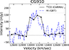 |
Fig. 6. H I emission taken from GBT observations (in blue). The CARMA spectrum is overplotted in black. The H I flux is scaled by a factor of 80 to facilitate a comparison. |
where Sν is the integrated flux density in units of Jy km s−1 and DMpc is the luminosity distance as 188 Mpc. A factor of 1.4 has been included to correct for the presence of helium. To obtain the integrated flux density, we determined the standard deviation of the flux in the emission-free channels and subtracted it from the main H I spectrum. Table 3 shows the integrated flux-density of H I, which is 0.4 ± 0.1 Jy km s−1. The mass error is also determined using the standard deviation of the emission-free channels. Hence, the derived mass of the main component of the galaxy is estimated as 3.1 ± 0.8 × 10⁹ M⊙. Kreckel et al. (2012) studied a sample of 41 void galaxies with their H I masses in the range of 1.7 × 10⁸ to 5.5 × 10⁹ M⊙. Our estimation is consistent with their sample. However, the atomic mass of CG 910, M(H I), is smaller than the molecular mass M(H2), which will be discussed further in a later section.
4.5. Star formation efficiency and specific star formation rate
The star formation efficiency (SFE) is calculated as SFR/M(H2), where the SFR is calculated using the Hα flux from the MANGA map. Using SFR of 0.33 M⊙ yr−1 and M(H2) of 12 × 109 M⊙, we calculated SFE = 0.27 × 10⁻¹⁰ yr−1. We also calculated the specific star formation rate (sSFR) as SFR/M★, where M★ is the stellar mass of the galaxy. Using the archival stellar mass of ∼21.5 × 10⁹ M⊙, we calculated the sSFR = 0.07 × 10⁻¹⁰ yr−1 (log sSFR = −10.82).
5. Discussion
We have studied the cold gas distribution (H2 and H I) in the Boötes Void galaxy CG 910, which had previously been detected in CO(1–0) line emission using the single-dish IRAM telescope (Sage et al. 1997). The results suggest that the molecular gas distribution is lopsided and asymmetrical around the nucleus (see Appendix A). The gradient in the velocity dispersion map is also similar to the direction of the extended gas morphology in the CO intensity map, suggesting that the gas distribution is disturbed. Molecular gas or CO maps of void galaxies are rare, and this is possibly the first CO map of a void galaxy. The molecular gas mass in the inner disk is also surprisingly high (M(H2) = 12 × 109 M⊙) compared to normal galaxies (Obreschkow & Rawlings 2009). Also, void galaxies are, in general, H I dominated (Szomoru et al. 1993, 1996), but in this case, we find that the H I gas mass is smaller than the H2 mass. This is surprising but not completely unusual (Beygu et al. 2013). Table 3 shows the details of the detected fluxes and gas masses in CG 910.
In normal environments such as galaxy clusters, a lower M(H I) can be due to gas stripping associated with frequent galaxy interactions and mergers, as the outer-lying H I gas is more easily stripped compared to the H2 gas that lies deep inside the disk. So, the main reason for M(H I) < M(H2) must be a slow SFR compared to the rate of conversion of H I to M(H2). To understand this further, we estimated the H2 gas depletion time, tdep (H2) = M(H2)/SFR, which is the timescale required for a galaxy to consume the whole molecular gas mass at the current SFR. With an M(H2) of 12 × 109 M⊙ and SFR of 0.33 M⊙ yr−1, we find that tdep(H2) ∼ 36 Gyr. The atomic gas depletion timescale, tdep(H I) = M(H I)/SFR, is the timescale over which the atomic mass is converted to stars at a given SFR, and we estimate the tdep(H I) to be ∼9.27 Gyr. This timescale is high compared to star-forming galaxies, for example, in the xCOLD GASS survey (Saintonge et al. 2017), but is approximately close to the quenched galaxies that have tdep (H I) > 10 Gyr (Guo et al. 2021). This value suggests that with its moderate SFR, CG 910 is forming stars over a relatively long timescale, thereby supporting the scenario of slow star formation in voids. Recent studies on void galaxies also suggest that the gas in voids is slowly assembled (Domínguez-Gómez et al. 2022, 2023).
Recent studies of massive star-forming galaxies (M★ = 109–1011.5 M⊙) in the xGASS survey (Catinella et al. 2018), and the ALMaQUEST (Yu et al. 2024) survey suggest that the variations in the molecular-to-atomic gas fraction are mostly driven by changes in the H I reservoirs, which are dependent on stellar mass surface densities. Although CG 910 is also a massive galaxy, the stellar and gas masses (M(H2) or M(H I)) are almost comparable, whereas, for most star-forming disk galaxies, the gas mass is < 10% of the stellar mass. This suggests that the stellar mass surface density in CG 910 may not be high enough to provide the self-gravity required to support global disk instabilities, such as bars and spiral arms. The latter’s dynamical processes are the main drivers of star formation in galaxies. A similar reasoning applies to low surface brightness galaxies, which have very diffuse stellar disks (Das 2013). Thus, this study suggests that CG 910, like most void galaxies (Kreckel et al. 2011), is slowly evolving and is still using up its gas content in star formation.
5.1. Comparison with the void galaxy survey CO-CAVITY
The largest void galaxy survey so far, called CO-CAVITY, studied the molecular line emission for 200 galaxies using IRAM 12CO (1-0) and 12CO(2-1) observations (Rodríguez et al. 2024), and included the pilot study of 20 void galaxies (Domínguez-Gómez et al. 2022). We compared the photometric and star formation properties of CG 910 (MH2, MHI, SFE, sSFR, MH2/MHI, MHI/M★) as shown in Table 4, with those of the sample. We find that CG 910 is redder (g-r = 0.89) and more luminous (Mr = −20.4) than most CO-CAVITY galaxies and lies at the upper brightness limit. Rodríguez et al. (2024) suggested that the star-formation properties of their void galaxy sample do not differ much from normal star-forming galaxies except at the high stellar mass end. The molecular hydrogen mass (log MH2) for the CO-CAVITY sample varies from 7.64 to 9.84. The authors derived the mean SFE in five different stellar mass bins (9.0 < log M★ < 11.5) and found that the SFE is constant with stellar mass and varies marginally from −8.94 to −8.99. The stellar and molecular mass of CG 910 lies at the higher end of the sample (log M★ = 10.33 and log MH2 = 10.079) when compared with the CO-CAVITY sample. The SFE for CG 91O (log SFE (yr−1) = − 10.56) is much lower than the overall distribution of the CO-CAVITY sample and falls in the higher stellar mass bin (M★ > 1010.5 M⊙). The mean sSFR ranges from −9.91 to −10.53, and so the sSFR of CG 910 (log sSFR = −10.82) is lower than the CO-CAVITY sample. For the molecular-to-atomic gas mass ratio, CG 910 (log MH2/MHI = 0.58) is consistent with galaxies in the higher stellar mass bin (M★ > 1010 M⊙) as stated in Domínguez-Gómez et al. (2022). The atomic gas mass fraction (log MHI/M★) of CG 910 is −0.84, lower than the average value in voids or for normal star-forming galaxies, but is consistent with the sample from CO-CAVITY.
Photometric and derived star formation properties of CG 910.
Environment of CG 910 taken from the GEMA catalogue.
5.2. Large-scale structure and the local environment of CG 910
Figure 7a displays the wedge diagram for the distribution of galaxies taken from the SDSS DR17 archive in the direction of Boötes Void. The red circle roughly marks the boundary of the void, considering it spherical with a radius of ∼50 Mpc (Kirshner et al. 1983), and the magenta star shows the location of CG910. The declination values stacked for the wedge plot range from 40°–50°. Panel (b) shows the RA-Dec distribution of the same sample of galaxies. The three-dimensional distribution of the galaxies showing RA, Dec and redshift for the redshift range of Boötes Void (0.04–0.06) is shown in panels (c) and (d) at azimuth angles of 110° and 40°, respectively. The green star shows the centre of Boötes Void and the red triangle marks the CG910 location. The open magenta circles show the nearest neighbours taken from the NED environment search tool1. The environment of galaxies is determined by two parameters: the density field (ηnn) and the tidal strength (Q), which allows for a clear picture of the effect of the environment of a galaxy. The gravitational potential is reconstructed by the mass density field of the galaxy groups in the SDSS survey (Wang et al. 2016). The tidal strength is defined as
 (3)
(3)
where p and i indices refer to the primary and neighbour galaxies, respectively. Dp is the diameter of the primary galaxy, M is the stellar mass of the galaxy, and di is the projected physical distance of the ith neighbour to the primary galaxy.
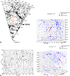 |
Fig. 7. (a) Wedge diagram showing the RA and redshift for the galaxies taken from the SDSS DR 17 archive with the stacked declination range of 40° and 50°. (b) Distribution of RA and Dec in the direction of the Boötes Void. The position of CG910 and the Boötes Void centre are marked. (c) Three-dimensional distribution of the environment around CG 910. Blue markers indicate the galaxies from the SDSS DR17 archive. The z-axis represents the respective redshift for each galaxy. The red triangle shows the location of CG910. The green star shows the central coordinates of the Boötes Void. The azimuth angle corresponds to 110°. (d) Distribution of galaxies in the same range of RA, Dec, and z at the azimuth angle of 40°. |
To quantify the local and large-scale environment of this galaxy, we used the parameters given in the Galaxy Environment for MaNGA (GEMA) Value-Added Catalogue2 (VAC; Argudo-Fernández et al., in prep.). Table 5 shows the number of nearest neighbours (nn) and the corresponding tidal strength of the nearest neighbour (Qnn) and large-scale structure (QLSS) with the projected density to the fifth nearest neighbour at 1 Mpc and 5 Mpc. The density within 1 Mpc is quite low, but the tidal strength is higher, whereas within the volume of 5 Mpc, the density as well as the tidal strength are both high. The presence of one single nearest neighbour at ∼250 kpc may explain the higher value of tidal strength with low number density, averaged over the three nearest neighbours. The large-scale environment can be characterised by using the eigenvalues of the tidal tensor along the major, intermediate and minor axes at the position of the galaxy (Hahn et al. 2007; Zheng et al. 2017). The eigenvalues taken from the GEMA catalogue for this galaxy are t1 = 0.14, t2 = −0.04, t3 = −0.68. This combination of eigenvalues with t1 > 0, t2 < 0 and t3 < 0 suggest that is a sheet-like environment (Wang et al. 2016). Argudo-Fernández et al. (2015, 2025) characterised the local and large-scale environment of the isolated galaxies using their three-dimensional distribution and found that the void galaxies are different from the isolated galaxies in filaments and walls.
One of the main reasons we studied this galaxy was to see if we could detect any ongoing gas accretion. This could be due to either interaction with close companion galaxies or cold gas accretion from the intergalactic medium via cosmic web filaments. A good way to search for gas accretion is to look for gas with abnormal velocities in the PV plot (Fig. 5). Signatures of interaction can also be detected in molecular gas and would appear as abnormal velocities in the PV plot. A good example of such an interaction is the void galaxy Mrk 1477 or VGS31 (Kreckel et al. 2012), which is part of a system of three interacting galaxies connected by a gas filament and shows significant CO emission (Beygu et al. 2013). However, we did not detect any abnormal gas velocities in the CO observations. The PV plot shows only a marginal detection towards the south-western side of the galaxy at a flux level of 0.05 Jy/beam. There is a hint of possible extended emission in the south-western direction of the galaxy, but considering the beam size of the CARMA data, this may or may not be real. Furthermore, optical images show no nearby companion galaxies that could trigger gas accretion, nor are there any signatures of a recent minor merger event in the galaxy. Thus, CG 910 shows no clear signatures of gas accretion in the CO data.
6. Conclusions
We present CO and H I observations of the galaxy CG 910, which lies in the Boötes Void. The CARMA CO(1–0) observations reveal that the molecular gas has a H2 mass of 12 ± 1.1 × 10⁹ M⊙ and is distributed in a disk with a diameter of 7 kpc. The CO velocity field shows a regularly rotating disk with a flat rotation velocity of 256 kms−1. The CO velocity dispersion and the CO intensity peak in the centre suggest that the gas is concentrated in the bulge region. The single-dish GBT observations of the H I spectrum show that the H I gas has a mass of 3.1 ± 0.8 × 10⁹ M⊙, is also centrally concentrated, and has a distribution similar to that of the molecular gas. We have spatially resolved the molecular gas properties of a void galaxy for the first time and attribute the low atomic gas mass fraction to the longer gas depletion timescale, confirming the slow evolution of the gas in voids. We do not find any substantial signatures of offset CO emission. There are hints of offset H I emission in the GBT H I spectrum, but the S/N is not high. Hence, we do not detect any clear signatures of gas accretion in the void galaxy CG 910.
Acknowledgments
The authors gratefully acknowledge the help of Prof. Stuart Vogel in obtaining the CARMA data and its analysis. We would like to express our sincere gratitude to Prof. Leslie Sage and Prof. Marc W. Pound for providing the 30m IRAM data on CG910. We thank the anonymous referee for his constructive comments, which have improved the science and clarity of the manuscript. This work is supported by the National Natural Science Foundation of China (NSFC) (Grant No. 12588202, 11988101) and by the Alliance of International Science Organisations, Grant No. ANSO-VF-2021-01. The first author, E.S., is grateful to IIA for hosting her two-month visit and for the financial support from the Science and Engineering Research Board (SERB) MATRICS grant MTR/2020/000266 for that period. PB gratefully acknowledges the support of the Science and Engineering Research Board (SERB) Core Research Grant CRG/2022/004531. D.L. is a new cornerstone investigator. MD also gratefully acknowledges the support of the SERB Core Research Grant CRG/2022/004531, and the Department of Science and Technology (DST) grant DST/WIDUSHI-A/PM/2023/25(G) for this research. ZZ is supported by the National Key R&D Program of China No. 2023YFC2206403 and 2024YFA1611602. ZZ is also supported by NSFC grants No. 12373012, 12041302 and CMS-CSST-2025-A08. This material is based upon work supported by the Green Bank Observatory, which is a major facility funded by the National Science Foundation and operated by Associated Universities, Inc. The paper is also based on observations done with the Combined Array for Research in Millimetre Astronomy (CARMA), which was funded by the National Science Foundation. The study has made use of the NASA Extragalactic Database (NED) and the SDSS survey. Funding for the Sloan Digital Sky Survey IV has been provided by the Alfred P. Sloan Foundation, the U.S. Department of Energy Office of Science, and the Participating Institutions. SDSS-IV acknowledges support and resources from the Center for High-Performance Computing at the University of Utah. The SDSS website is www.sdss4.org. SDSS-IV is managed by the Astrophysical Research Consortium for the Participating Institutions of the SDSS Collaboration including the Brazilian Participation Group, the Carnegie Institution for Science, Carnegie Mellon University, Center for Astrophysics | Harvard & Smithsonian, the Chilean Participation Group, the French Participation Group, Instituto de Astrofísica de Canarias, The Johns Hopkins University, Kavli Institute for the Physics and Mathematics of the Universe (IPMU) / University of Tokyo, the Korean Participation Group, Lawrence Berkeley National Laboratory, Leibniz Institut für Astrophysik Potsdam (AIP), Max-Planck-Institut für Astronomie (MPIA Heidelberg), Max-Planck-Institut für Astrophysik (MPA Garching), Max-Planck-Institut für Extraterrestrische Physik (MPE), National Astronomical Observatories of China, New Mexico State University, New York University, University of Notre Dame, Observatário Nacional / MCTI, The Ohio State University, Pennsylvania State University, Shanghai Astronomical Observatory, United Kingdom Participation Group, Universidad Nacional Autónoma de México, University of Arizona, University of Colorado Boulder, University of Oxford, University of Portsmouth, University of Utah, University of Virginia, University of Washington, the University of Wisconsin, Vanderbilt University, and Yale University. This study has made use of Astropy, a community-developed core Python (http://www.python.org) package for Astronomy (Astropy Collaboration 2013, 2018, 2022); ipython (Perez & Granger 2007); matplotlib (Hunter 2007); SciPy, a collection of open-source software for scientific computing in Python (Virtanen et al. 2020); pandas, an open source data analysis and manipulation tool (pandas development team 2020; McKinney 2010) NumPy, a structure for efficient numerical computation (van der Walt et al. 2011).
References
- Alatalo, K., Blitz, L., Young, L. M., et al. 2011, ApJ, 735, 88 [NASA ADS] [CrossRef] [Google Scholar]
- Alatalo, K., Davis, T. A., Bureau, M., et al. 2013, MNRAS, 432, 1796 [NASA ADS] [CrossRef] [Google Scholar]
- Alpaslan, M., Robotham, A. S. G., Driver, S., et al. 2014, MNRAS, 438, 177 [Google Scholar]
- Aragón-Calvo, M. A., van de Weygaert, R., & Jones, B. J. T. 2010, MNRAS, 408, 2163 [CrossRef] [Google Scholar]
- Argudo-Fernández, M., Verley, S., Bergond, G., et al. 2015, A&A, 578, A110 [NASA ADS] [CrossRef] [EDP Sciences] [Google Scholar]
- Argudo-Fernández, M., Duarte Puertas, S., & Verley, S. 2025, A&A, 695, A256 [NASA ADS] [CrossRef] [EDP Sciences] [Google Scholar]
- Astropy Collaboration (Robitaille, T. P., et al.) 2013, A&A, 558, A33 [NASA ADS] [CrossRef] [EDP Sciences] [Google Scholar]
- Astropy Collaboration (Price-Whelan, A. M., et al.) 2018, AJ, 156, 123 [Google Scholar]
- Astropy Collaboration (Price-Whelan, A. M., et al.) 2022, ApJ, 935, 167 [NASA ADS] [CrossRef] [Google Scholar]
- Beygu, B., Kreckel, K., van de Weygaert, R., van der Hulst, J. M., & van Gorkom, J. H. 2013, AJ, 145, 120 [NASA ADS] [CrossRef] [Google Scholar]
- Beygu, B., Peletier, R. F., van der Hulst, J. M., et al. 2017, MNRAS, 464, 666 [NASA ADS] [CrossRef] [Google Scholar]
- Biswas, P., Patra, N. N., Roy, N., & Rashid, M. 2022, MNRAS, 513, 168 [Google Scholar]
- Bolatto, A. D., Wolfire, M., & Leroy, A. K. 2013, ARA&A, 51, 207 [CrossRef] [Google Scholar]
- Boomsma, R., Oosterloo, T. A., Fraternali, F., van der Hulst, J. M., & Sancisi, R. 2008, A&A, 490, 555 [NASA ADS] [CrossRef] [EDP Sciences] [Google Scholar]
- Bos, E. G. P., van de Weygaert, R., Dolag, K., & Pettorino, V. 2012, MNRAS, 426, 440 [NASA ADS] [CrossRef] [Google Scholar]
- Catinella, B., Saintonge, A., Janowiecki, S., et al. 2018, MNRAS, 476, 875 [NASA ADS] [CrossRef] [Google Scholar]
- Ceccarelli, L., Herrera-Camus, R., Lambas, D. G., Galaz, G., & Padilla, N. D. 2012, MNRAS, 426, L6 [Google Scholar]
- Chengalur, J. N., & Pustilnik, S. A. 2013, MNRAS, 428, 1579 [NASA ADS] [CrossRef] [Google Scholar]
- Conrado, A. M., González Delgado, R. M., García-Benito, R., et al. 2024, A&A, 687, A98 [NASA ADS] [CrossRef] [EDP Sciences] [Google Scholar]
- Constantin, A., Hoyle, F., & Vogeley, M. S. 2008, ApJ, 673, 715 [NASA ADS] [CrossRef] [Google Scholar]
- Cruzen, S. T., Weistrop, D., & Hoopes, C. G. 1997, AJ, 113, 1983 [Google Scholar]
- Cruzen, S., Wehr, T., Weistrop, D., Angione, R. J., & Hoopes, C. 2002, AJ, 123, 142 [Google Scholar]
- Curtis, O., McDonough, B., & Brainerd, T. G. 2024, ApJ, 962, 58 [NASA ADS] [CrossRef] [Google Scholar]
- Das, M. 2013, JApA, 34, 19 [Google Scholar]
- Das, M., Saito, T., Iono, D., Honey, M., & Ramya, S. 2015, ApJ, 815, 40 [NASA ADS] [CrossRef] [Google Scholar]
- Das, S., Sardone, A., Leroy, A. K., et al. 2020, ApJ, 898, 15 [NASA ADS] [CrossRef] [Google Scholar]
- Domínguez-Gómez, J., Lisenfeld, U., Pérez, I., et al. 2022, A&A, 658, A124 [NASA ADS] [CrossRef] [EDP Sciences] [Google Scholar]
- Domínguez-Gómez, J., Pérez, I., Ruiz-Lara, T., et al. 2023, Nature, 619, 269 [CrossRef] [Google Scholar]
- Egorova, E. S., Moiseev, A. V., & Egorov, O. V. 2019, MNRAS, 482, 3403 [CrossRef] [Google Scholar]
- Guo, H., Jones, M. G., Wang, J., & Lin, L. 2021, ApJ, 918, 53 [NASA ADS] [CrossRef] [Google Scholar]
- Hahn, O., Porciani, C., Carollo, C. M., & Dekel, A. 2007, MNRAS, 375, 489 [NASA ADS] [CrossRef] [Google Scholar]
- Hoffman, Y., & Shaham, J. 1982, ApJ, 262, L23 [NASA ADS] [CrossRef] [Google Scholar]
- Huchra, J., Davis, M., Latham, D., & Tonry, J. 1983, ApJS, 52, 89 [NASA ADS] [CrossRef] [Google Scholar]
- Hunter, J. D. 2007, Comput. Sci. Eng., 9, 90 [NASA ADS] [CrossRef] [Google Scholar]
- Kennicutt, R. C., Jr., Tamblyn, P., & Congdon, C. E. 1994, ApJ, 435, 22 [Google Scholar]
- Kirshner, R. P., Oemler, A., Schechter, P. L., & Shectman, S. A. 1983, in Early Evolution of the Universe and Its Present Structure, eds. G. O. Abell, & G. Chincarini, IAU Symp., 104, 197 [Google Scholar]
- Kleiner, D., Pimbblet, K. A., Jones, D. H., Koribalski, B. S., & Serra, P. 2017, MNRAS, 466, 4692 [Google Scholar]
- Kreckel, K., Platen, E., Aragón-Calvo, M. A., et al. 2011, AJ, 141, 4 [NASA ADS] [CrossRef] [Google Scholar]
- Kreckel, K., Platen, E., Aragón-Calvo, M. A., et al. 2012, AJ, 144, 16 [Google Scholar]
- Libeskind, N. I., van de Weygaert, R., Cautun, M., et al. 2018, MNRAS, 473, 1195 [NASA ADS] [CrossRef] [Google Scholar]
- Marganian, P., Garwood, R. W., Braatz, J. A., Radziwill, N. M., & Maddalena, R. J. 2013, Astrophysics Source Code Library [record ascl:1303.019] [Google Scholar]
- McKinney, W. 2010, in Proceedings of the 9th Python in Science Conference, eds. S. van der Walt, & J. Millman, 56 [Google Scholar]
- Nadathur, S., & Percival, W. J. 2019, MNRAS, 483, 3472 [NASA ADS] [CrossRef] [Google Scholar]
- Obreschkow, D., & Rawlings, S. 2009, MNRAS, 394, 1857 [NASA ADS] [CrossRef] [Google Scholar]
- pandas development team, T. 2020, https://doi.org/10.5281/zenodo.3509134 [Google Scholar]
- Pandey, D., Saha, K., & Pradhan, A. C. 2021, arXiv e-prints [arXiv:2107.01774] [Google Scholar]
- Perez, F., & Granger, B. E. 2007, Comput. Sci. Eng., 9, 21 [Google Scholar]
- Pustilnik, S. A., Martin, J. M., Lyamina, Y. A., & Kniazev, A. Y. 2013, MNRAS, 432, 2224 [Google Scholar]
- Roberts, M. S. 1962, AJ, 67, 437 [NASA ADS] [CrossRef] [Google Scholar]
- Rodríguez, M. I., Lisenfeld, U., Duarte Puertas, S., et al. 2024, A&A, 692, A125 [NASA ADS] [CrossRef] [EDP Sciences] [Google Scholar]
- Rodríguez-Medrano, A. M., Springel, V., Stasyszyn, F. A., & Paz, D. J. 2024, MNRAS, 528, 2822 [CrossRef] [Google Scholar]
- Rojas, R. R., Vogeley, M. S., Hoyle, F., & Brinkmann, J. 2004, ApJ, 617, 50 [NASA ADS] [CrossRef] [Google Scholar]
- Román, J., Beasley, M. A., Ruiz-Lara, T., & Valls-Gabaud, D. 2019, MNRAS, 486, 823 [CrossRef] [Google Scholar]
- Russell, E. 2014, MNRAS, 438, 1630 [Google Scholar]
- Sage, L. J., Weistrop, D., Cruzen, S., & Kompe, C. 1997, AJ, 114, 1753 [NASA ADS] [CrossRef] [Google Scholar]
- Saintonge, A., Catinella, B., Tacconi, L. J., et al. 2017, ApJS, 233, 22 [Google Scholar]
- Sancisi, R., Fraternali, F., Oosterloo, T., & van der Hulst, T. 2008, A&ARv, 15, 189 [NASA ADS] [CrossRef] [Google Scholar]
- Sault, R. J., Teuben, P. J., & Wright, M. C. H. 1995, in Astronomical Data Analysis Software and Systems IV, eds. R. A. Shaw, H. E. Payne, & J. J. E. Hayes, ASP Conf. Ser., 77, 433 [Google Scholar]
- Sheth, R. K., & van de Weygaert, R. 2004, MNRAS, 350, 517 [NASA ADS] [CrossRef] [Google Scholar]
- Shim, J., Park, C., Kim, J., & Hwang, H. S. 2021, ApJ, 908, 211 [Google Scholar]
- Solomon, P. M., & Vanden Bout, P. A. 2005, ARA&A, 43, 677 [NASA ADS] [CrossRef] [Google Scholar]
- Szomoru, A., van Gorkom, J. H., Gregg, M., & de Jong, R. S. 1993, AJ, 105, 464 [Google Scholar]
- Szomoru, A., van Gorkom, J. H., & Gregg, M. D. 1996, AJ, 111, 2141 [Google Scholar]
- van de Weygaert, R., & Platen, E. 2011, Int. J. Mod. Phys. Conf. Ser., 1, 41 [NASA ADS] [CrossRef] [Google Scholar]
- van der Walt, S., Colbert, S. C., & Varoquaux, G. 2011, Comput. Sci. Eng., 13, 22 [Google Scholar]
- Vielzeuf, P., Kovács, A., Demirbozan, U., et al. 2021, MNRAS, 500, 464 [Google Scholar]
- Virtanen, P., Gommers, R., Oliphant, T. E., et al. 2020, Nat. Methods, 17, 261 [Google Scholar]
- Wang, H., Mo, H. J., Yang, X., et al. 2016, ApJ, 831, 164 [Google Scholar]
- Weistrop, D., Hintzen, P., Kennicutt, R. C., Jr., et al. 1992, ApJ, 396, L23 [Google Scholar]
- Weistrop, D., Hintzen, P., Liu, C., et al. 1995, AJ, 109, 981 [Google Scholar]
- Winkel, B., Kraus, A., & Bach, U. 2012, A&A, 540, A140 [NASA ADS] [CrossRef] [EDP Sciences] [Google Scholar]
- York, D. G., Adelman, J., Anderson, J. E., Jr., et al. 2000, AJ, 120, 1579 [NASA ADS] [CrossRef] [Google Scholar]
- Yu, N., Zheng, Z., Tsai, C.-W., et al. 2024, Sci. China Phys. Mech. Astron., 67, 299811 [Google Scholar]
- Zheng, Z., Wang, H., Ge, J., et al. 2017, MNRAS, 465, 4572 [Google Scholar]
Appendix A: Asymmetric distribution of intensity in the molecular hydrogen disk
To quantify the asymmetry in 12CO emission or in molecular H2 disk between the two halves of the galaxy due to the probable presence of the extended emission in the right half, we adopted the following approach. Contours were drawn on the moment zero map at levels of (1, 2, 4, 6, 8, 10, 12)×RMSmom0, where RMSmom0 is the RMS noise of the moment zero map. The regions enclosed between each pair of successive contours were bisected along the galaxy’s position angle, defining left and right halves. We then computed the total emission separately for each half within every such region. The results of this analysis are presented in Fig. A.1.
From Fig. A.1b, a significant emission asymmetry is observed in Region 5, defined between the fifth (4σ) and sixth (2σ) contours, with the innermost contour considered as the first. In this region, the difference in emission between the right and left halves is 14.7 ± 2.0 Jy/beam-km/s. In contrast, all other regions exhibit negligible differences (i.e. ∼0). This scenario illustrates the asymmetric distribution, or lopsided phenomenon, of the molecular hydrogen disk.
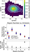 |
Fig. A.1. Measuring the asymmetry of the molecular hydrogen disk. Panel (a): 12CO moment zero map of the galaxy. The white contours represent surface brightness levels of (1, 2, 4, 6, 8, 10, 12)Jy/beam-km/s. The red line indicates the position angle of the galaxy and bisects each region, defined between two successive contours, into left and right halves. The corresponding total emission measured separately from each half as a function of region number is presented in panel (b). Top of panel (b): Total emission from the left and right halves of the galaxy plotted for each successive region between two contours. Region 1 corresponds to the area within the innermost contour. Subsequent regions (Region 2, 3, 4, etc) are defined between successive contours, moving outwards. Bottom of panel (b): Difference in total emission between the right and left halves (right – left) for each region. The horizontal dashed line marks zero difference, serving as a reference to illustrate the asymmetry of the two halves. |
All Tables
All Figures
|
Fig. 1. SDSS r-band image of CG 910. |
| In the text | |
|
Fig. 2. Channel maps for CG 910 based on 12CO (1-0) data. The velocity in the first panel is 12 746.3 km s−1, with a velocity resolution of −81.2 km s−1. Contour levels are set at 6.5 × (1, 1.4, 2, 2.8, 4, 5.6, 8, 11.2, 16, 22.4, 32, 44.8, 64) mJy/beam, where 6.5 mJy/beam represents the RMS noise at a line-free channel of the data cube. |
| In the text | |
|
Fig. 3. 12CO (1-0) moment maps of CG 910. In panel (a), the red contours, which represent the 12CO emission, are plotted over the SDSS r-band image. The contours are set at (1, 2, 4, 8...) mJy/beam-km/s sigma levels. In panel (b), contours are set at 20 km s−1 intervals. The red patch at the bottom-left corner of each image represents the beam of the 12CO map. |
| In the text | |
|
Fig. 4. 12CO spectra extracted from CARMA observations (in black) and IRAM 30 m single-dish observations (in green; Sage et al. 1997). |
| In the text | |
|
Fig. 5. PV diagram along different slices of the galaxy. The white contours are drawn at RMS × (1, 1.4, 2, 2.8, 4, 5.6, 8, ...) levels; the RMS is measured from a line-free channel of the 12CO data cube. |
| In the text | |
|
Fig. 6. H I emission taken from GBT observations (in blue). The CARMA spectrum is overplotted in black. The H I flux is scaled by a factor of 80 to facilitate a comparison. |
| In the text | |
|
Fig. 7. (a) Wedge diagram showing the RA and redshift for the galaxies taken from the SDSS DR 17 archive with the stacked declination range of 40° and 50°. (b) Distribution of RA and Dec in the direction of the Boötes Void. The position of CG910 and the Boötes Void centre are marked. (c) Three-dimensional distribution of the environment around CG 910. Blue markers indicate the galaxies from the SDSS DR17 archive. The z-axis represents the respective redshift for each galaxy. The red triangle shows the location of CG910. The green star shows the central coordinates of the Boötes Void. The azimuth angle corresponds to 110°. (d) Distribution of galaxies in the same range of RA, Dec, and z at the azimuth angle of 40°. |
| In the text | |
|
Fig. A.1. Measuring the asymmetry of the molecular hydrogen disk. Panel (a): 12CO moment zero map of the galaxy. The white contours represent surface brightness levels of (1, 2, 4, 6, 8, 10, 12)Jy/beam-km/s. The red line indicates the position angle of the galaxy and bisects each region, defined between two successive contours, into left and right halves. The corresponding total emission measured separately from each half as a function of region number is presented in panel (b). Top of panel (b): Total emission from the left and right halves of the galaxy plotted for each successive region between two contours. Region 1 corresponds to the area within the innermost contour. Subsequent regions (Region 2, 3, 4, etc) are defined between successive contours, moving outwards. Bottom of panel (b): Difference in total emission between the right and left halves (right – left) for each region. The horizontal dashed line marks zero difference, serving as a reference to illustrate the asymmetry of the two halves. |
| In the text | |
Current usage metrics show cumulative count of Article Views (full-text article views including HTML views, PDF and ePub downloads, according to the available data) and Abstracts Views on Vision4Press platform.
Data correspond to usage on the plateform after 2015. The current usage metrics is available 48-96 hours after online publication and is updated daily on week days.
Initial download of the metrics may take a while.