| Issue |
A&A
Volume 706, February 2026
|
|
|---|---|---|
| Article Number | A376 | |
| Number of page(s) | 13 | |
| Section | Extragalactic astronomy | |
| DOI | https://doi.org/10.1051/0004-6361/202555290 | |
| Published online | 23 February 2026 | |
The impact of selection criteria on the properties of green valley galaxies
1
Department of Physics, Mbarara University of Science and Technology P. O. Box 1410 Mbarara, Uganda
2
MSPE Department, School of Education, College of Education, University of Rwanda P. O. Box 55 Rwamagana, Rwanda
3
Instituto de Astrofísica de Andalucía (IAA-CSIC) Glorieta de la Astronomía s/n 18008 Granada, Spain
4
Astronomy and Astrophysics Department, Entoto Observatory and Research Center (EORC), Space Science and Geospatial Institute (SSGI) P. O. Box 33679 Addis Ababa, Ethiopia
5
South African Astronomical Observatory (SAAO) P. O. Box 9 Observatory Cape Town 7935, South Africa
6
Southern African Large Telescope (SALT) P. O. Box 9 Observatory Cape Town 7935, South Africa
★ Corresponding author: This email address is being protected from spambots. You need JavaScript enabled to view it.
Received:
24
April
2025
Accepted:
18
December
2025
Abstract
Context. The bi-modality in the distribution of galaxies usually obtained from colour-colour or colour-stellar mass (absolute magnitude) diagrams has been studied to determine the difference between galaxies in the blue cloud and in the red sequence, as well as to define the green valley region. As a transition region, green valley galaxies can offer clues about the morphological transformation of galaxies from late-type to early-type. Therefore, the selection of green valley samples is of fundamental importance.
Aims. In this work, for the first time, we evaluate the selection effects of the most frequently applied green valley selection criteria. The aim is to understand how these criteria affect the identification of green valley galaxies, their properties, and their impact on galaxy evolution studies.
Methods. Using the SDSS optical and GALEX ultraviolet data at redshift z < 0.1, we selected the eight most commonly used criteria based on colours (without and with Gaussian fittings), specific star formation rate, and star formation rate versus stellar mass. We then studied the properties of the green valley galaxies (e.g. their stellar mass, star formation rate, specific star formation rate, intrinsic brightness, and morphological and spectroscopic types) for each selection criterion.
Results. We found that when using different criteria, we selected different types of galaxies. UV-optical colour-based criteria tend to select more massive galaxies, with lower star formation rates and a higher fractions of composite and elliptical galaxies than when using pure optical colours. Our results also show that the colour-based criteria are the most sensitive to galaxy properties, rapidly changing the selection of green valley galaxies.
Conclusions. Whenever possible, we suggest avoiding the green valley colour-based selection and using other methods or a combination of several, such as the star formation rate versus stellar mass or specific star formation rate.
Key words: galaxies: active / galaxies: evolution / galaxies: formation / galaxies: fundamental parameters / galaxies: star formation / galaxies: statistics
© The Authors 2026
 Open Access article, published by EDP Sciences, under the terms of the Creative Commons Attribution License (https://creativecommons.org/licenses/by/4.0), which permits unrestricted use, distribution, and reproduction in any medium, provided the original work is properly cited.
This article is published in open access under the Subscribe to Open model. This email address is being protected from spambots. You need JavaScript enabled to view it. to support open access publication.
1. Introduction
The distribution of galaxies in colour–stellar mass (M*), colour–magnitude, colour–star formation rate (SFR), or SFR–M* diagrams show two over-density regions at both low and high redshift. These over-density regions are called the red sequence and the blue cloud (e.g. Strateva et al. 2001; Baldry et al. 2004; Salim et al. 2007; Brammer et al. 2009; Pović et al. 2013; Lee et al. 2015; Combes 2016; Nogueira-Cavalcante et al. 2018; Phillipps et al. 2019; Sampaio et al. 2022; Noirot et al. 2022). In general, the red sequence is mainly populated by quiescent galaxies with early-type morphologies, but it also contains dusty star-forming and edge-on spiral galaxies, while the blue cloud mainly hosts star-forming galaxies rich in gas and dust and with late-type morphologies, along with a small fraction of early-type galaxies with recent star formation and/or active galactic nuclei (e.g. Pović et al. 2013; Tojeiro et al. 2013; Schawinski et al. 2014; Jian et al. 2020; Donevski et al. 2023; Paspaliaris et al. 2023; Le Bail et al. 2024). The green valley, located between the red sequence and the blue cloud, is a sparsely populated region with a significantly smaller number of galaxies, at least in the UV-optical-NIR surveys (e.g. Salim 2014; Bremer et al. 2018; Phillipps et al. 2019; Jian et al. 2020; Noirot et al. 2022). It was suggested that green valley galaxies could represent the transition population between the blue cloud of star-forming galaxies and the red sequence of quenched and passive galaxies (e.g. Martin et al. 2007; Salim et al. 2007; Schiminovich et al. 2007; Wyder et al. 2007; Pan et al. 2013; Salim 2014; Lee et al. 2015; Smethurst et al. 2015; Coenda et al. 2018; Angthopo et al. 2019, 2020; de Sá-Freitas et al. 2022; Smith et al. 2022; Estrada-Carpenter et al. 2023; Mazzilli Ciraulo et al. 2024; Das & Pandey 2025). In the SFR-M* plane, the green valley can be described as the region located below the main sequence of star formation (e.g. Noeske et al. 2007; Chang et al. 2015; Ilbert et al. 2015; Abdurro’uf & Akiyama 2018; Belfiore et al. 2018; Jian et al. 2020; Sampaio et al. 2022; Koprowski et al. 2024).
Green valley galaxies account for approximately 10–20% of galaxies in all environments (e.g. Schawinski et al. 2014; Jian et al. 2020; Das et al. 2021). In most previous studies at both low and intermediate redshifts (z < 1.5), the green valley galaxies represent an intermediate population, with their properties (e.g. luminosity, stellar mass, SFRs, stellar ages, stellar populations, etc.) ranging between those of red sequence and blue cloud galaxies (e.g. Salim et al. 2007; Pan et al. 2013; Schawinski et al. 2014; Lee et al. 2015; Smethurst et al. 2015; Trayford et al. 2015; Coenda et al. 2018; Phillipps et al. 2019). They contain intermediate distributions of structural parameters such as the Sérsic index, concentration parameters, asymmetry, smoothness, and bulge-to-total flux ratio (e.g. Schiminovich et al. 2007; Mendez et al. 2011; Mahoro et al. 2019). However, certain inconsistencies have been found in previous works regarding morphologies of green valley galaxies, reporting spirals to be between 70–95% and the elliptical galaxies to account for 5–30%, depending on the specific study (e.g. Salim 2014; Bait et al. 2017; Lin et al. 2017; Das et al. 2021; Aguilar-Argüello et al. 2025). Inconsistencies have also been found when studying the environments of green valley galaxies, reporting a range of strong to mild environmental effects, as well as a lack of dependence on the environment. For example, some works suggested that stellar mass, SFR, stellar age, the fraction of AGNs, and the morphology of green valley galaxies are all unaffected by their environments (e.g. Schawinski et al. 2014; Starkenburg et al. 2019; Jian et al. 2020; Das et al. 2021). Meanwhile, others found that the properties of green valley galaxies are environment-dependent (e.g. Coenda et al. 2018). Regarding the AGN properties, X-ray, and optical studies found a larger fraction of AGNs in the green valley (up to z < 2), suggesting that AGN feedback might be important for star formation quenching in the green valley (e.g. Nandra et al. 2007; Hasinger 2008; Silverman et al. 2008; Pović et al. 2012; Cimatti et al. 2013; Leslie et al. 2016; Lacerda et al. 2020; Das et al. 2021). However, when considering FIR emitters in the green valley, enhanced SFRs have been found in active in comparison to non-active galaxies, independently of morphology, suggesting possible signs of positive AGN feedback (e.g. Mahoro et al. 2017, 2019, 2022, 2023).
For the morphological transformation of galaxies within the green valley, different timescales have been proposed, from short (< 1 Gyr) and intermediate (1–2 Gyr) to slow quenching (> 2 Gyr) (e.g. Faber et al. 2007; Balogh et al. 2011; Schawinski et al. 2014; Lee et al. 2015; Smethurst et al. 2015; Nogueira-Cavalcante et al. 2018; Gu et al. 2018; Phillipps et al. 2019; Angthopo et al. 2019; Kacprzak et al. 2021; Estrada-Carpenter et al. 2023). In addition, various studies offered a scenario assuming a distinct evolution of cosmic gas supply and gas reservoirs, concluding that early- and late-type galaxies take significantly different evolutionary paths to and through the green valley. It has been suggested that early-type galaxies undergo a rapid quenching of star formation (< 250 Myr), passing through the green valley as quickly as stellar evolution allows. Late-type galaxies, on the other hand, go through a slow decline in star formation (> 1 Gyr) and a gradual departure from the main sequence (e.g. Schawinski et al. 2014; Bremer et al. 2018; Kelvin et al. 2018; Eales et al. 2018; Bryukhareva & Moiseev 2019; Wu et al. 2020; Quilley & de Lapparent 2022). Different processes of star formation quenching have been suggested to play a role in the green valley, from inside-out (e.g. Zewdie et al. 2020) to outside-in (e.g. Starkenburg et al. 2019).
Several selection criteria were previously used to define the green galaxy, including colour-based methods such as U − V (e.g. Brammer et al. 2009), U − B (e.g. Mendez et al. 2011; Mahoro et al. 2017, 2019), NUV − r (e.g. Wyder et al. 2007; Salim et al. 2007; Salim 2014; Lee et al. 2015; Coenda et al. 2018; de Sá-Freitas et al. 2022; Noirot et al. 2022), g − r (e.g. Trayford et al. 2015; Walker et al. 2013; Eales et al. 2018), u − r (e.g. Bremer et al. 2018; Eales et al. 2018; Kelvin et al. 2018; Ge et al. 2019; Phillipps et al. 2019); SFR-based methods such as: sSFR (e.g. Schiminovich et al. 2007; Salim et al. 2009; Salim 2014; Phillipps et al. 2019; Starkenburg et al. 2019), SFR–M* diagram (e.g. Noeske et al. 2007; Chang et al. 2015; Pandya et al. 2017; Jian et al. 2020; Sampaio et al. 2022), or Dn4000 index (e.g. Angthopo et al. 2019, 2020); or, in some cases, hybrid methods, which mix the above properties like colour-colour diagrams, colour vs. sSFR diagram, etc. (Salim 2014, and references therein). Some other criteria based on infrared data, full spectral energy distribution (SED) fitting or star formation quenching indicators have been used in the literature (e.g, Mahoro et al. 2017; Brownson et al. 2020; Noirot et al. 2022; Mahoro et al. 2023; Villanueva et al. 2024); however, many of them are extensions or refinements of the other criteria mentioned above (e.g. Mahoro et al. 2017, 2023). As can be seen, colour criteria have been the most used in previous studies, mainly by visual selection and, in some cases, by Gaussian fitting of colour distribution. It has been suggested that NUV − r colour outperforms the u − r and g − r colours in the selection of green valley galaxies because the black-body radiation spectra of young stellar populations peak in the NUV, resulting in a higher dynamic range and hence improved separation in the usual colours of red sequence and blue cloud (e.g. Gu et al. 2018). However, despite the fact that there are numerous criteria, no study has yet examined their selection effects and tried to understand how and if the inconsistent results obtained in previous studies (and mentioned above) might be related to the green valley selection. This work aims to study for the first time the eight most used green valley selection criteria based on optical SDSS and UV GALEX data (colour without and with Gaussian fitting (g − r, NUV − r), sSFR, and SFR-M* criteria) to better understand the properties of the selected galaxies and the impact of tested criteria on the results obtained previously (e.g. Salim et al. 2009; Walker et al. 2013; Salim 2014; Trayford et al. 2015; Eales et al. 2018; Sampaio et al. 2022, and references therein). These eight criteria are considered the most widely used and to be standard ones, as they appear frequently in the literature (e.g. Schawinski et al. 2014; Coenda et al. 2018; Bremer et al. 2018), in particular, in all-sky SDSS-GALEX studies at low redshift (e.g. Bremer et al. 2018; Turner et al. 2021). In selecting these eight criteria, we include different green valley selection methods, as mentioned above (e.g. between the 1D and 2D parameter space).
From now on, the paper is organised as follows: In Section 2, we present the data used. Section 3 discusses sample selection and different green valley selection criteria. Section 4 summarises the main analysis and results of this work. In Section 5, we discuss the implications of our results, while the summary and conclusions are presented in Section 6. We assume the following cosmological parameters throughout the paper: Ωm = 0.3 and ΩΛ = 0.7, with H0 = 70 km s−1 Mpc−1. The AB system was used to calculate all the magnitudes in this study.
2. Data
In this work, we used optical and UV data. In the optical, we used the data from Sloan Digital Sky Survey (SDSS) (York et al. 2000) Data Release 7 (DR7, Abazajian et al. 2009). In particular, we used the MPA-JHU1 catalogue of 927552 sources, with the available measurements of emission line fluxes, stellar masses, and SFRs used in Sections 3 and 4. The extracted stellar masses were measured through a fit to the spectral energy distribution (SED) by using the SDSS broad-band optical photometry (Kauffmann et al. 2003). The Hα emission-line luminosity was used to determine the SFRs for the star-forming galaxies as classified in the BPT diagram and was corrected for dust extinction (Brinchmann et al. 2004). For all other galaxies, either AGN or non-emission-line galaxies, the SFRs were inferred from the D4000–SFR relation (Brinchmann et al. 2004). For having a complete sample in the SDSS, we selected all galaxies with redshift z < 0.1 (Netzer 2009). This resulted in a sample of 381798 galaxies, hereafter referred to as the ‘optical sample’.
The UV data were extracted from the GALEX-AIS (GR5) catalogue of 6.5 million sources down to a magnitude of 19.9 and 20.8 in FUV and NUV, respectively (Martin et al. 2005). We used in particular the NUV data, centred at 2300 Å. Bianchi et al. (2014) found that the SDSS data depth matches well the GALEX-AIS catalogue used in this work. Using a radius of 2 arcsec, we cross-matched the optical and UV catalogues and obtained a total sample of 179419 galaxies, hereafter referred to as the ‘UV sample’.
3. Green valley selection criteria
In this work, we analysed and compared, for the first time, the eight commonly used green valley selection criteria. Using both optical and UV samples, we selected colour-based methods, such as g − r and NUV − r, with the green valley selected visually and by the Gaussian fitting, as well as SFR-based methods, such as sSFR and SFR-M*. We selected these eight criteria because they are standard and have been the most frequently used in previous works with SDSS and GALEX data in the low-redshift universe (e.g. Schawinski et al. 2014; Coenda et al. 2018; Bremer et al. 2018; Turner et al. 2021); however, an investigation of their reliability and comparison of the selected galaxies have not been carried out before. While additional criteria exist in the literature, their application has been either less common and/or is limited by incomplete data coverage. The number of green valley galaxies selected with each of the tested criteria is given in Table 1. Detailed information regarding the different selection criteria is provided in Sections 3.1–3.4 in optically and UV-selected green valley galaxies.
Number of green valley galaxies obtained using eight standard selection criteria.
3.1. Colour-based methods
3.1.1. g − r criterion (C1)
The first criterion we selected in our analysis is the g − r rest-frame colour in optical (hereafter, C1; e.g. Trayford et al. 2015; Walker et al. 2013; Eales et al. 2018). We obtained the rest-frame colour through the K-corrected magnitudes using TOPCAT2 (Taylor 2013, 2017). Overall, 90% of all sources have g and r magnitude errors below 5%. The distribution of g − r rest-frame colour for all galaxies selected in optical is shown in Fig. 1. Taking into account the distribution of all galaxies, we defined (using purely a visual inspection) the green valley as the region between the two peaks, corresponding to the blue cloud and the red sequence, with 0.63 < g − r < 0.75. This is indicated in Fig. 1 with the dashed vertical lines. Using this criterion, 78959 (∼21%) of the 381798 galaxies were selected as part of the green valley sample.
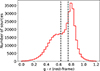 |
Fig. 1. Distribution of g − r rest-frame colour for the optical sample. The two black dashed lines define the green valley region, with the red sequence peak (on the left) and the blue cloud peak (on the right). |
Our definition C1 of green valley is comparable with previous studies. For example, Trayford et al. (2015) used the galaxies from the EAGLE survey at z < 0.1 and, by using the same rest-frame colour, they defined the green valley as 0.6 < g − r < 0.75. Belfiore et al. (2018) used the MaNGA sample and similarly defined the green valley as 0.61 < g − r < 0.71 in the redshift range of 0.01 < z < 0.15. Walker et al. (2013) used the same criterion, defining the green valley as 0.55 < g − r < 0.70, using a relatively small sample of SDSS galaxies.
The literature emphasises that the green valley is generally identified as the region between the two peaks (blue cloud and red sequence) in the colour distribution of galaxies, but the exact boundaries may vary and are often subjective (e.g. Salim 2014; Angthopo et al. 2020; Pandey 2024). To clarify, the visual boundaries chosen here are based on the balance between: 1) a pure visual inspection and the balance between the general distribution of the two peaks in the colour distribution and 2) a comparison with previous works in the literature (particular those considering the same redshift range for the samples) to ensure that the boundaries are consistent with previous studies. Since the main objective of this work is not to study or propose new selection criteria for green valley galaxies, but to better understand and compare the selection effects and properties of green valley galaxies previously selected using different (and most commonly used) criteria. Although our visually determined green valley may be subjective, the boundaries are broadly consistent with previous studies and, thus, consistent with our main objective. However, when testing for and avoiding the impact of this subjectivity, we also aim to test more quantitative criteria using Gaussian fitting, as described in Section 3.4.
3.1.2. NUV − r criterion (C2)
Colours based on the NUV and optical photometric bands are commonly used to select the green valley (e.g. Lee et al. 2015; Coenda et al. 2018; Noirot et al. 2022) and, in particular, the NUV − r colour, which is a sensitive tracer of recent star formation activity. Using our UV sample, the NUV − r bi-modal colour distribution is shown in Fig. 2. For the same reasons given in Section 3.1.1, we defined the green valley visually, between the peaks of the blue cloud and the red sequence. It is located between the two vertical dashed lines as a region between the two peaks defined as 3 < NUV − r < 4. Using this criterion, we obtained 18 230 (∼10%) green valley galaxies (out of a total UV sample of 179419 galaxies).
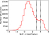 |
Fig. 2. Distribution of the NUV − r colour for the UV sample. The green valley is defined between the two dashed lines. |
Several previous studies have used similar criteria and visual identification to select the green valley, depending on the redshift. Mendez et al. (2011) used a green valley sample selected from the All-Wavelength Extended Growth Strip International Survey (AEGIS) at redshift of z < 1.2 using the NUV − r rest-frame colours and the range of 3.2 < NUV − r < 4.1. Salim (2014) used non-dust-corrected SDSS and GALEX data at z < 0.22 and the green valley was selected within the range of 4 < NUV − r < 5 in the UV-optical rest-frame colour, while Salim et al. (2009) selected the green valley using the range of 3.5 < NUV − r < 4.5 in the rest-frame, non-dust corrected colours at the redshift of z < 1.4. In addition, Belfiore et al. (2018) used the MaNGA catalogue and defined the green valley galaxies using the UV-optical rest-frame colour and the ranges of 4 < NUV − r < 5 at the redshift of 0.01 < z < 0.15. de Sá-Freitas et al. (2022) used the SDSS DR12 at the redshift of 0.05 ≤ z ≤ 0.095 and defined the green valley in the range of 2.8 < NUV − r < 3.5.
3.2. SFR-based methods
3.2.1. SFR-M* criterion in the optical (C3)
The SFR-M* diagram was also commonly used to select the green valley galaxies, as a region between the star-forming and passive galaxies without active star formation going on (e.g. Chang et al. 2015; Curtis-Lake et al. 2021; Kalinova et al. 2021; Vilella-Rojo et al. 2021). We used the SFR-M* diagram as our third criterion (hereafter C3) to select the green valley galaxies, by plotting the density contours to highlight regions of varying galaxy concentrations where the over-density contours reveal two prominent peaks corresponding to the star-forming and quiescent populations. The green valley is then defined empirically where the density contours show a minimum in the number density, as shown in Fig. 3, and in line with Schawinski et al. (2014). With this in mind, we selected the green valley region between the two dashed lines defined as
![Mathematical equation: $$ \begin{aligned} \log \,\text{ SFR}\,[\text{ M}_{\odot }/\text{ yr}]& = 0.80 *\log \,(\text{ M}_{*}[\text{ M}_{\odot }]) - 9.155, \end{aligned} $$](/articles/aa/full_html/2026/02/aa55290-25/aa55290-25-eq1.gif) (1)
(1)
![Mathematical equation: $$ \begin{aligned} \log \,\text{ SFR}\,[\text{ M}_{\odot }/\text{ yr}]& = 0.80 *\log \,(\text{ M}_{*}[\text{ M}_{\odot }]) - 8.599. \end{aligned} $$](/articles/aa/full_html/2026/02/aa55290-25/aa55290-25-eq2.gif) (2)
(2)
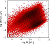 |
Fig. 3. SFR-M* diagram for an optical sample of galaxies. The green valley is defined between the two dashed lines. These lines were determined by plotting the density contours in the galaxy distribution. |
between the two clear over-density regions of the blue cloud (above the selected green valley region) and the red sequence (below the green valley). Using C3, we selected 54 187 (∼14%) green valley galaxies in optical. Our selection and Eqs. (1) and (2) correspond to several previous studies, including Belfiore et al. (2018), Starkenburg et al. (2019), Jian et al. (2020), and Sampaio et al. (2022).
3.2.2. SFR-M* criterion in UV (C4)
We defined the fourth criterion to our UV sample as SFR-M* to determine the green valley region, as shown in Fig. 4. We followed the same procedure as in Section 3.2.1 and defined the green valley using the density contours as an area between the two overpopulated regions of the blue cloud and the red sequence with a minimum in number density, marked between the dashed lines using Eqs. (3) and (4) as
![Mathematical equation: $$ \begin{aligned} \log \,\text{ SFR}\,[\text{ M}_{\odot }/\text{ yr}]& = 0.75 *\log \,(\text{ M}_{*}[\text{ M}_{\odot }]) - 8.88, \end{aligned} $$](/articles/aa/full_html/2026/02/aa55290-25/aa55290-25-eq3.gif) (3)
(3)
![Mathematical equation: $$ \begin{aligned} \log \,\text{ SFR}\,[\text{ M}_{\odot }/\text{ yr}]& = 0.75 *\log \,(\text{ M}_{*}[\text{ M}_{\odot }]) - 8.2. \end{aligned} $$](/articles/aa/full_html/2026/02/aa55290-25/aa55290-25-eq4.gif) (4)
(4)
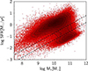 |
Fig. 4. SFR versus stellar mass for the UV sample. The green valley is defined between the two dashed lines. |
We obtained 17 871 (10%) green valley galaxies in total using this criterion. Our selection is in line with previous studies (e.g. Noeske et al. 2007; Lee et al. 2015).
3.3. sSFR-based methods
3.3.1. SFR criterion in optical (C5)
The sSFR was used commonly in previous works to select the green valley galaxies (e.g. Schiminovich et al. 2007; Salim et al. 2009; Salim 2014; Phillipps et al. 2019; Starkenburg et al. 2019). The distribution of sSFR for the optical sample is shown in Fig. 5. In line with the justification given in Section 3.1, the green valley sample was selected visually between the two peaks and is represented by the black dashed lines, covering the range of −11.6 < sSFR < −10.6. Using this criterion (hereafter, C5), we selected a total of 84 753 (∼22%) green valley galaxies.
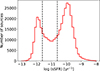 |
Fig. 5. sSFR distribution for the optical sample. The green valley lies between the two vertical dashed lines. |
Our selection is consistent with previous studies based on sSFR distribution and visual selection. In Salim (2014), using also the SDSS data at z < 0.22, the green valley was selected as −11.8 < log(sSFR) < −10.8, while the range of −11.0 < log(sSFR) < −10.0 was used in Salim et al. (2009). Phillipps et al. (2019) used the data from the GAMA survey at a redshift of 0.1 < z < 0.2 and defined the green valley using sSFR in the range of −11.5 < log(sSFR) < −10.6. On the other hand, using Illustris3 and EAGLE4 simulations at z = 0, Starkenburg et al. (2019) defined the green valley galaxies using the sSFR in the range of −13.0 < sSFR < −10.5.
3.3.2. sSFR criterion in UV (C6)
The selection of green valley galaxies using the sSFR in UV is similar to the one in optical described in Section 3.3.1 and is shown in Fig. 6. Using the same criterion visually identified as in optical, we selected 30884 green valley galaxies (∼17%). In Salim et al. (2009) and Salim (2014), the authors used the same selection criteria, suggesting that the green valley selection using the sSFR does not change significantly independently of the colour used.
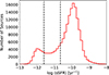 |
Fig. 6. Distribution of the sSFR in the UV sample. The green valley is defined between the two dashed lines. |
3.4. Gaussian-fitting based methods
3.4.1. Gaussian fitting on g − r colour distribution criterion (C7)
To avoid visual selection, several previous works used the two Gaussian functions to simultaneously fit the distributions of the blue cloud and the red sequence when different colours are used, as well as to define the galaxies in the green valley between the two Gaussian peaks (e.g. Baldry et al. 2004; Wyder et al. 2007; Mendez et al. 2011; Krause et al. 2013; Parente et al. 2025). In this work, to compare visually and not-visually selected green valley galaxies in the colour-based methods, we performed an additional analysis for the g − r criterion by simultaneously fitting the bi-modal distribution with two Gaussian components via a simple least-squares fitting. After obtaining the best-fit parameters, we de-blended the Gaussian components to obtain the two individual Gaussians corresponding to the blue cloud and red sequence. This approach is similar to the criterion used by Parente et al. (2025) when fitting u − r optical colours, where they defined the green valley to be in the region within μB + σB to μR − σR (subscripts B and R refer to the blue cloud and red sequence, respectively), where μ and σ represent the mean and standard deviation, respectively, of each Gaussian fit. However, among other conditions, their definition of the green valley requires that μR − σR ≥ xBR and μB + σB ≤ xBR, where xBR is the intersection of the two Gaussian components. This method uses Gaussian fits to the observed colour distribution (i.e. a statistical approach to modeling the underlying populations) and the means and standard deviations are derived from the data, while the intersection is mathematically determined. Since using a single mean and standard deviation was not properly selecting the green valley among our sample, we modified and redefined the green valley as the region falling within ![Mathematical equation: $ \frac{1}{2}\left[\left(\mu_R + \mu_B\right) + \left(\sigma_B + \sigma_R\right)\right] $](/articles/aa/full_html/2026/02/aa55290-25/aa55290-25-eq5.gif) and
and ![Mathematical equation: $ \frac{1}{2}\left[\left(\mu_R + \mu_B\right) - \left(\sigma_B + \sigma_R\right)\right] $](/articles/aa/full_html/2026/02/aa55290-25/aa55290-25-eq6.gif) , using the average values of μ and σ of the two Gaussian fits instead of using a single mean and standard deviation. Figure 7 shows the double-component Gaussian fit (black solid line), the individual components for the blue cloud (blue dashed line), and the red sequence (red dashed line). The vertical black dashed lines define the green valley region in g − r colour between the values of 0.6–0.77, similarly to what we report in Section 3.1.1. Following this criterion, we selected 116 150 (∼30%) green valley galaxies.
, using the average values of μ and σ of the two Gaussian fits instead of using a single mean and standard deviation. Figure 7 shows the double-component Gaussian fit (black solid line), the individual components for the blue cloud (blue dashed line), and the red sequence (red dashed line). The vertical black dashed lines define the green valley region in g − r colour between the values of 0.6–0.77, similarly to what we report in Section 3.1.1. Following this criterion, we selected 116 150 (∼30%) green valley galaxies.
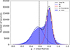 |
Fig. 7. g − r colour and simultaneous double Gaussian fit criterion. The black solid line represents the best fit. The blue and red dashed Gaussians show individual components which correspond to the blue cloud and the red sequence, respectively. The green valley region is shown between the two dashed black vertical lines. |
3.4.2. Gaussian fitting on NUV − r colour distribution criterion (C8)
Similarly to what we describe in Section 3.4.1, to avoid the subjectivity associated with visually identified green valley galaxies, we performed a Gaussian fit to the NUV − r colour distribution. We defined the green valley region by fitting the bi-modal distribution simultaneously with two Gaussian components, as described in Section 3.4.1. Figure 8 shows the double-component fit (black solid line) and the individual components of the blue cloud (blue dashed line) and the red sequence (red dashed line). The green valley region is defined between the two vertical black dashed lines covering the range of values in the NUV − r colour of 1.5–3.4. This resulted in a sample of 55 438 (∼31%) green valley galaxies.
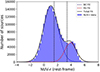 |
Fig. 8. Distribution of the NUV − r colour and Gaussian fittings of the blue cloud (blue dashed line) and the red sequence (red dashed line). The green valley is defined between the two black dashed vertical lines. |
4. Data analysis and results
In this section, we present some of the key properties of green valley galaxies when selected using the eight different criteria described in Sections 3.1–3.4, including the stellar mass, SFRs, sSFRs, intrinsic brightness, morphology, and spectroscopic types of galaxies. We also discuss the possible impact of extinction on our results.
4.1. Stellar mass
The stellar mass distribution of all optically (top panel) and UV-selected (bottom panel) green valley galaxies is shown in Fig. 9. The median values (vertical lines in both figures) of log (M*) are 10.31, 10.43, 10.45, 10.31, [M⊙] for optically selected green valley galaxies using criteria C1, C3, C5, and C7, respectively, along with 10.57, 10.53, 10.52, 10.36 [M⊙] in the UV using criteria C2, C4, C6, and C8, respectively. The Q1–Q35 values for all criteria are given in Table 2. As can be seen in Fig. 9, the stellar mass distributions in optical are similar for C1 and C7, being lower than in C3 and C5. Similar is the case in UV, with now slightly lower masses obtained for C8 than for C2, C4, and C6. In general, the differences in both the optical and UV between the four selection criteria are, on average, of an order of up to log (M*) = ± 0.14 [M⊙] in the optical and of up to log (M*) = ± 0.2 [M⊙] in UV (between C8 and other three UV criteria). On the other hand, when comparing colour (without and with Gaussian fit), sSFR, and SFR-M* criteria between optical and UV in Fig. 9 and statistics given in Table 2, it can be seen that the UV green valley criteria tend to select slightly more massive galaxies. The difference is most significant in the colour criterion case (without the Gaussian fitting) compared to other criteria. For this criterion, in the optical, 50% of the sources occupy the log M* range of 10.07–10.51 [M⊙] with a mean of 10.31 [M⊙], compared to 50% of the galaxies in the green valley in UV, which lie between 10.28–10.83 [M⊙] and have a mean of 10.57 [M⊙]. These differences become less significant in the case of other three criteria, as can be seen in Fig. 9 and Table 2. An analysis of the two-sample Kolmogorov-Smirnov (KS) test for the stellar masses of different optically and UV-selected samples indicates that, in all cases, the two samples do not come from the same parent distribution (p-value < 0.05). The difference is more pronounced for the colour criterion (without Gaussian fitting) compared to the other criteria, where the D-parameter6 is 29%, compared to 11%, 6.5%, and 9.2% for criteria C7 versus C8, C5 versus C6, and C3 versus C4, respectively.
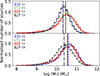 |
Fig. 9. Comparison of stellar mass for optically (top panel) and UV-selected (bottom panel) green valley galaxies using colour (C1 (g − r) and C2 (NUV − r), blue dashed histograms), SFR-M* (C3 and C4, red solid histograms, sSFR (C5 and C6, green dotted histograms), and colour with Gaussian fit (C7 (g − r) and C8 (NUV − r), black dot-dashed histograms)) criteria. The vertical dashed lines in both panels represent the median values of each criterion applied. |
log (M*) statistics in units of [M⊙] in the eight green valley criteria.
4.2. Star formation rates
Figure 10 shows the distribution of the SFRs of all green valley samples and their corresponding median values. As in the previous section, when comparing the four criteria in the optical, we find that C1 and C7 show similar distributions, with larger SFRs than C3 and C5 (see Table 3). On the other hand, for the UV sample, C8 shows a different distribution, with higher SFRs than C2, C4, and C6. As in the case of the stellar mass, the colour criteria without Gaussian fit show the largest difference between the optically selected and the UV-selected green valley galaxies. When using the C1 criterion, the galaxies show a median log (SFR) of −0.13 [M⊙ yr−1], where 50% of the sources lie between −0.83 - 0.26 [M⊙ yr−1], compared to the C2 criterion where green valley galaxies display lower values of log (SFR) with 50% of galaxies being in the range of −1.07 – (−0.15) [M⊙ yr−1] with a median of −0.69 [M⊙ yr−1]. Differences are less significant for the other three criteria, as can be seen in Table 3. The two distributions are again the most similar when sSFR criteria are used. As is the case with stellar mass, the two-sample KS test showed that the two samples, optical, and UV, do not come from the same parent distribution (p-value < 0.05) in the case of all criteria, with the more pronounced difference seen in terms of the colour criteria (without Gaussian fitting) of D = 27%.
log (SFR) statistics in units of [M⊙ yr−1] in the eight green valley criteria.
4.3. Specific SFRs
We tested the log (sSFR) of selected green valley samples by analysing the distribution of every sample and measuring their statistics. Fig. 11 shows the distribution of sSFR in optical (top panel) and UV (bottom panel) samples, along with their corresponding medians. The medians of log (sSFR) in our samples are −10.39, −10.92, −11.12, and −10.40 [yr−1] for the green valley selected in the optical using the C1, C3, C5, and C7 criteria, respectively, and −11.22, −11.18, −11.00, and −10.32 [yr−1] for the green valley selected in UV using C2, C4, C6, and C8 criteria, respectively. When comparing the four criteria in the selected optical and UV samples, we found similar trends as in the case of stellar mass and SFRs, with C1 and C7 having similar distributions, compared to C3 and C5 in the optical, and with the largest differences between C8 and the other three criteria in the UV. When comparing the same criteria between the optical and UV samples, the difference is again the most significant for the colour criteria without Gaussian fitting, with the median of −10.39 (and Q1–Q3 range of −10.96 – −10.14) for C1 and −11.22 (Q1–Q3 range of −11.74 – −10.67) for C2. These differences are less significant in the case of the other three criteria, as can be seen in Table 4. The results from the two-sample KS test revealed that in all cases, when comparing the same criteria in the optical and UV, the two samples do not come from the same parent distribution (p-value < 0.05), with the colour criterion (no Gaussian fit) again showing the largest difference, with D = 40%, compared to other criteria where D is lower (12%, 10%, 32% for C7 versus C8, C5 versus C6, and C3 versus C4, respectively).
log (sSFR) statistics in units of [yr−1] in the eight green valley criteria.
4.4. Absolute magnitude, Mr
We analysed the absolute magnitude in the r band (Mr) to compare the intrinsic brightness of the optical and UV samples. The median values of Mr are −19.64, −19.75, −19.77, and −19.63 for the optical sample using C1, C3, C5, and C7 criteria, respectively, and −20.12, −19.99, −19.80, and −19.85 for the C2, C4, C6, and C8 criteria, respectively, in the UV. Fig. 12 represents the distribution of absolute magnitude in the r band (Mr) obtained in all green valley selected optical (top) and UV (bottom) samples. The main statistics of all distributions are provided in Table 5. We observe that green valley galaxies selected in the UV are intrinsically slightly brighter than galaxies selected using optical criteria. Similar as in the above cases, the KS test showed that the two samples are not from the same parent distribution (all p-values are < 0.05). As is the case with the previously discussed parameters, the difference is more pronounced in colour criteria without any Gaussian fitting (D = 23%) compared to other criteria where D is 10%, 2%, and 9% for colour with Gaussian fit, sSFR, and SFR versus M*, respectively.
Mr statistics in the eight green valley criteria.
4.5. Morphological types
Morphology is a powerful indicator of a galaxy’s dynamical and merger history, playing a crucial role in understanding the evolutionary pathways of green valley galaxies. It is strongly correlated with many physical parameters, including mass, star formation, and star formation history (e.g. Schawinski et al. 2014; Pović et al. 2012; Smith et al. 2022; Estrada-Carpenter et al. 2023). In this section, we analyse the morphological classification of all green valley galaxies selected using different criteria.
We used the visual morphological classification from the Galaxy Zoo citizen science project Lintott et al. (2008, 2011) where galaxies were classified as: spiral, elliptical, and uncertain based on their structure. The ‘uncertain’ classification includes galaxy mergers and interactions, edge-on galaxies, peculiar galaxies, and unknown morphologies. Galaxies categorised as ‘elliptical’ or ‘spiral’ require that 80% of Galaxy Zoo users to have classified it in that category, after the debiasing technique was carried out. All remaining galaxies are then categorised as uncertain (the CLEAN technique; Land et al. 2008). After cross-matching the Galaxy Zoo catalogue with our catalogues of green valley optical and UV samples, we obtained the morphological classifications for each criterion, shown in Fig. 13. Table 6 shows the statistics in % of all morphological types, where the percentages in column 2 were obtained by comparing the number of galaxies after cross-matching with Galaxy Zoo and the number of galaxies in the original green valley samples.
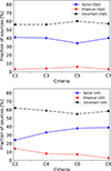 |
Fig. 13. Comparison of morphological classification of green valley samples for every criterion ranging from C1, C3, C5, and C7 for optically selected sample (top panel) and C2, C4, C6, and C8 for UV-selected sample (bottom panel). The morphological types are from the Galaxy Zoo survey. The blue solid line, red dotted line, and the black dash-dotted line represent spiral, elliptical, and uncertain (unclassified) galaxies, respectively. |
As can be seen in both Fig. 13 and Table 6, we detected, in all criteria, more spiral galaxies than than elliptical ones in the green valley. This is not surprising since most of the previous morphological studies (at both low and intermediate redshifts) confirmed that the population of late-type galaxies is higher than that of early-types (see e.g. Nair & Abraham 2010; Pović et al. 2013). On the other hand, the system of classification, together with the quality of SDSS images, is responsible for an excessive number of uncertain sources. When comparing the fractions of elliptical and spiral galaxies in the optical and UV samples, the only significant difference is between the two colour criteria without Gaussian fitting (C1 versus C2), where we selected more spiral galaxies (41% vs. 24%, respectively) than elliptical (3% versus 14%, respectively) in the optical and UV, as seen in Table 6.
Morphological classification using Galaxy Zoo (Lintott et al. 2008, 2011) where Sp is for spiral, Ell is for elliptical, and Unc is for uncertain.
4.6. Spectroscopic types
We analysed the selection of different spectroscopic types in the green valley when using different criteria in the optical and the UV. Using the BPT diagram (log ([O III] λ5007/Hβ) versus log ([N II]/Hα)) defined in Baldwin et al. (1981), we were able to classify the galaxies in our samples into star-forming, composite galaxies, Seyfert 2, and LINERs. We selected sources with a signal-to-noise ratio of S/N > 3 in all four lines ([O III] λ5007, Hβ, Hα, and [N II] λ6584). We used the following references to previous works to separate the different classes: Kauffmann et al. (2003) to separate star-forming and composite galaxies; Kewley et al. (2001) to separate composite and AGN galaxies; and Schawinski et al. (2007) to separate Seyfert 2 and LINERs. In Table 7 we present the statistics for our spectroscopic classification, where the percentages in column 2 were calculated by comparing the number of sources obtained after considering the S/N > 3 in all four lines with the number of original green valley samples. In Fig. 14, we give a comparison of the optically (top panel) and UV-selected (bottom panel) samples.
Spectroscopic classification of the green valley selected samples into star-forming galaxies (SF), composites (Com), Seyfert 2 (Sey), and LINERs.
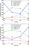 |
Fig. 14. Distribution of spectroscopic types for green valley galaxies selected using different optical (top) and UV (bottom) criteria. We present the star-forming galaxies (blue solid line), composite galaxies (green dotted line), Seyfert 2 (red dash-dotted line), and LINERs (black dashed line). |
Most of the galaxies in the green valley are classified as star-forming or composite in the case of most criteria. When comparing the optical and the UV criteria, the main difference is between C1 and C2, colour criteria without Gaussian fitting, with star-forming galaxies being the most selected in the C1 criterion and composite galaxies in the C2 criterion. For the colour criteria with Gaussian fit (C7 and C8), star-forming galaxies are dominant in both criteria without significant difference, as can be seen in Table 7.
4.7. Effect of extinction on the green valley selection
The selection of the green valley using the colour criteria may be affected by dust extinction. Since the previously defined colour selection criteria (C1, C2, C7, and C8) did not consider any dust extinction, we studied its possible effect in this section. One of the most reliable techniques to estimate dust extinction is through the Hα/Hβ flux ratio (i.e. the Balmer decrement), which has been commonly used, in particular in the local Universe (Domínguez et al. 2013). We define the dust extinction from the Balmer decrements following the steps described in Pović et al. (2016).
In Fig. 15, we show the C1 (top) and C2 (bottom) criteria before (in red) and after (in blue) applying the dust extinction correction. As can be seen, the two distributions are significantly different, both in the overall distribution and in the number of sources in the green valley. In particular, the number of sources is significantly different, and many sources are lost after applying the extinction correction because either Hα, Hβ, or both lines are not strong and/or not present in the SDSS galaxy spectra. Elliptical galaxies are more affected by the extinction correction than spirals, as they do not have strong emission lines (i.e. after correcting for extinction, we tend to lose more elliptical galaxies than spiral galaxies). This affects the bi-modal distribution of galaxies, as seen in Figure 15, and the definition of the green valley for the extinction-corrected samples as well.
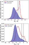 |
Fig. 15. Mg-Mr (top panel) and MNUV-Mr (bottom panel) colour distributions before (red histograms) and after (blue semi-filled histograms) the extinction correction. The green valley region defined in Sections 3.1.1 and 3.1.2 is represented by two vertical black-dashed lines. |
Using the same green valley galaxy selection criteria as used in Sections 3.1.1 and 3.1.2, we find that the extinction correction is affecting the green valley selection, as mentioned above. Using the Mg- Mr criterion, we selected 28 696 galaxies in the green valley (7.8%), compared to 74 663 (20%) galaxies that were in the green valley before the extinction correction. There are 1649 (0.5%) galaxies that were in the green valley before and remained in after correcting for extinction. Using the MNUV- Mr criterion, we went on to obtain 7546 galaxies in the green valley (4%), compared to 18 230 (10%) galaxies that were in the green valley before correcting for extinction. We have 1146 (0.65%) galaxies that were selected as green valley galaxies before and remained in the green valley after the extinction correction.
5. Discussion
Our results show that the selection of green valley using different criteria in optically and UV-selected samples introduces differences in the number of selected sources and their properties in terms of stellar mass, SFRs, sSFRs, intrinsic brightness, and the morphological and spectroscopic types. In all cases, using the KS test, we find that the optical and UV samples have different properties. The largest difference in properties is associated with the colour criteria, in particular, without applying Gaussian fittings; whereas the criteria based on the sSFR, and SFR versus M* display smaller variations in the properties of the optical and UV samples. Therefore, we recommend the use of the sSFR or the SFR versus M* criteria for the selection of the green valley. If these parameters are not available and colours are used instead, we recommend selecting the green valley using Gaussian fittings of the bi-modal galaxy distribution, rather than a visually determined green valley to avoid subjectivity.
Overall, the fraction of green valley galaxies obtained in this work using the colour (without Gaussian fittings), sSFR, and SFR versus M* criteria in the case of optical and UV samples is in line with previous results suggesting that green valley galaxies account for approximately 10–20% of galaxies in all environments (e.g. Schawinski et al. 2014; Jian et al. 2020; Das et al. 2021). However, using the colour criteria with Gaussian fittings leads to a higher fraction of green valley galaxies of ∼30% in the case of both optical and UV samples, as can be seen in Table 1. The selection of the green valley by the Gaussian fitting can also change when considering different ranges of absolute magnitudes (or stellar masses), as shown in previous studies (e.g. Wyder et al. 2007; Jin et al. 2014).
The stellar mass shows a slight difference between the optically and UV-selected green valley galaxies, with the UV sample having, on average, more massive galaxies compared to the optical samples using the same criteria, along with a slightly higher fraction of elliptical galaxies (see Table 6). This is consistent with the findings of Sobral et al. (2018), who suggested that the most massive O and B stars with lifetimes of a few Myr generate continuous UV radiation, and with the results of Sawicki (2012), who found a linear correlation between the stellar mass of galaxies and their UV luminosity. According to these studies, the most massive galaxies, being the main contributors to the aforementioned massive stars, could exhibit a high UV luminosity. In addition, the selection of more massive galaxies in the UV than in the optical also leads to the selection of more galaxies that are intrinsically brighter, as discussed in Section 4.4.
Our analysis was extended by classifying green valley samples morphologically and spectroscopically. The morphological classification based on the Galaxy Zoo (Lintott et al. 2008, 2011) shows that spiral galaxies are more dominant than elliptical galaxies in all green valley-selected samples, regardless of whether optically or UV-selected data were used. This is in line with previous green valley studies, which reported a higher fraction of spiral galaxies than ellipticals (e.g. see Das et al. 2021, and references therein). It is also in line with previous suggestions that elliptical and spiral galaxies have significantly different evolutionary paths to and through the green valley, with elliptical galaxies transiting faster through the green valley than spirals, leading to a larger fraction of spiral galaxies (e.g. Schawinski et al. 2014; Bremer et al. 2018; Bryukhareva & Moiseev 2019; Quilley & de Lapparent 2022). However, previous studies also show inconsistencies, as well as a broad range in the number of spiral and elliptical galaxies in the green valley, reporting spirals to be between 70–95% and the elliptical galaxies to account for 5–30%, depending on the study (e.g. Salim 2014; Bait et al. 2017; Lin et al. 2017; Das et al. 2021; Aguilar-Argüello et al. 2025). From our analysis, we can see that these inconsistencies in fractions among different studies can be explained by the use of either optical or UV-selected samples and different green valley criteria. As can be seen in Table 6, depending on the criterion, we selected 3–6% (34–41%) and 7–14% (24–38%) of elliptical (spiral) galaxies in the optical and UV, respectively, when considering the total sample, with many galaxies remaining unclassified in the Galaxy Zoo. However, if considering all classified galaxies, the above fractions become 7–15% (85–93%) and 16–37% (63–84%) of elliptical (spiral) galaxies in the optical and UV, respectively.
We found a range of different distributions in the SFRs (and, thus, in the sSFRs as well) depending on the optical or UV samples and the criteria used, as discussed in Sections 4.2 and 4.3. This can be explained by the selection of different fractions of elliptical and spiral galaxies, depending on the criteria as shown above, but also by different fractions of spectroscopic types selected by each criterion. In particular, the selection of star-forming galaxies being dominant in C1, C7, and C8 (above 60% in all cases), over the selection of composite galaxies being dominant in C3 and C5 in optical, and C2, C4, and C6 in the UV, with 40–50%. The fraction of Seyfert 2 galaxies, ∼4–10% is the lowest for almost all criteria, followed by LINERs from ∼4–25% depending on the criterion. This could explain again the diversity of previous findings regarding the star formation properties of galaxies in the green valley (e.g. Schiminovich et al. 2007; Damen et al. 2009; Pan et al. 2013; Schawinski et al. 2014; Chang et al. 2015; Coenda et al. 2018; Guo et al. 2021; Quilley & de Lapparent 2022), suggesting different scenarios from slow quenching, extended quenching due to mergers and star formation, up to fast quenching due to starbursts, with and without significant impact of AGN feedback on star formation (e.g. Zewdie et al. 2020; Kalinova et al. 2021).
In addition to the 1D and 2D colour-based and SFR-based methods discussed here, some studies have applied hybrid methods to select the green valley, suggesting that they could be more refined to identify green valley galaxies (e.g. Salim 2014). This includes combining colour-based and/or SFR-based methods, such as colour-colour (e.g. NUV − r vs. g − r) or colour-sSFR (e.g. NUV − r vs. sSFR) diagrams. The underlying idea is that these hybrid methods can help to disentangle the effects of dust attenuation and young and old stellar populations, thereby reducing misclassifications due to dust reddening. However, these approaches require high-quality and well-calibrated photometric data to minimise uncertainties and ensure robust results (e.g. Salim 2014; Pandey 2024) and, in addition, might decrease the number of sources in the sample and introduce more complexity in the selection of the green valley. As an example, we show in Figs. 16 and 17, the NUV − r versus g − r and NUV − r versus sSFR diagrams, respectively, for our sample. The lines drawn in the two figures show different possibilities of selecting the green valley according to the two galaxy over-densities and, thus, the complexity of the two plots. Given all of the above, most previous studies have typically defined the green valley using a single criterion, either colour-based or SFR-based, rather than combining several diagnostics, which can lead to inconsistencies between studies (e.g. Salim 2014; Pandey 2024). Therefore, in this work, we only considered the C1-C8 criteria, which are standard and the most used in previous works. The analysis of other criteria could be the subject of future work.
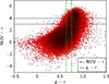 |
Fig. 16. Colour-colour criterion, with the possibility of green valley selection using either the g − r (green dot-dashed lines) or the NUV − r (black dashed lines) colours. |
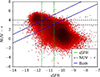 |
Fig. 17. NUV − r vs. sSFR relation, with the green valley selected with either the sSFR criterion (green dash-dotted lines), NUV − r criterion (black dashed lines), or mixed criteria (blue solid lines). |
Overall, our results suggest that the green valley is not a single population but a diverse class of galaxies at different evolutionary stages, depending on the selection criterion used. This is in line with some of the previous studies (e.g. Schawinski et al. 2014; Smethurst et al. 2015; Bremer et al. 2018; Nogueira-Cavalcante et al. 2018; Das et al. 2021; Lin et al. 2022; Smith et al. 2022; Lin et al. 2024; Das & Pandey 2025). To obtain a comprehensive view of the green valley galaxy evolution, both optical and UV selection methods should be combined, enabling the study of the full spectrum of quenching processes.
6. Conclusions
In this work, we compare, for the first time, the eight most commonly used green valley selection criteria and analysed the properties of the selected galaxies, as well as how they might affect the results reported in previous studies. To our knowledge, this is the first study of its kind and the most detailed, which should benefit future studies on green valley galaxies and their selection. We used the SDSS optical and GALEX UV data at z < 0.1 to analyse the properties of galaxies in different green valley samples selected based on optical and NUV colours (without and with Gaussian fittings), sSFR, and SFR versus M* criteria. We analysed the properties of selected galaxies from one criterion to another. The main findings are that green valley galaxies selected using different criteria in optical and UV may present different types of galaxies in terms of their M*, SFR, sSFR, intrinsic brightness, morphology, and spectroscopic type. Therefore, this should be taken into account in all green valley studies that normally use only a single selection criterion when interpreting the results obtained. Our main results are as follows:
-
The stellar mass of the green valley galaxies is slightly higher and the galaxies are intrinsically brighter when selected in the UV than in optical. They show very different SFRs and sSFRs depending on the criteria used.
-
In general, independently of optical and UV data, spirals are more dominant than elliptical galaxies in the green valley. However, the fraction of spiral and elliptical galaxies changes in optical (85–93% and 7–15%, respectively) and UV (63–84% and 16–37%, respectively), depending on the applied criterion.
-
Different criteria in the optical and the UV have tendencies of selecting either more star-forming or more composite galaxies, followed by LINERs and, finally, Seyfert 2 galaxies.
-
The dust extinction can significantly affect the green valley selection based on colours in both the optical and UV, in particular, due to the loss of galaxies with fully absent or weak emission lines.
-
The criteria of the green valley selection based on the g − r colours in the optical and NUV − r in the UV are the most sensitive to the galaxy properties. We found other sample selection criteria based on sSFR and the SFR versus M* to be more stable and more likely to be recommended given their ease of use. If the colour criteria are to be used, we recommend selecting the green valley through the Gaussian fitting of the bi-modal distribution of galaxies, rather than visually selecting the green valley, to avoid subjectivity.
Finally, our results suggest that the green valley is not a single population, but a diverse class of galaxies at different evolutionary stages, depending on the sample and the selection criterion used. To obtain a complete view of galaxy evolution through the green valley, both optical and UV selection methods should be combined, allowing the study of the full spectrum of quenching processes.
Data availability
This work is predominantly based on the public data from the Sloan Digital Sky Survey (SDSS) available at https://wwwmpa.mpa-garching.mpg.de/SDSS/DR7/, GALEX data from the Galaxy Evolution Explorer All Sky Imaging Surveys (GALEX-AIS) available at https://archive.stsci.edu/pub/hlsp/bianchi_gr5xdr7/. And data from Galaxy Zoo catalogue available at https://data.galaxyzoo.org/
Acknowledgments
We thank the anonymous referee for all his/her comments, which have improved our manuscript. Financial support from the Swedish International Development Cooperation Agency (SIDA) through the International Science Programme (ISP)-Uppsala University to the University of Rwanda through the Rwanda Astrophysics, Space and Climate Science Research Group (RASCSRG), and through the East African Astrophysics Research Network (EAARN) is gratefully acknowledged. MP acknowledges financial support from the Spanish MCIU through the project PID2022-140871NB-C21 by “ERDF A way of making Europe” and the project PID2024-162972NB-I00, the Severo Ochoa grant CEX2021-515001131-S funded by MCIN/AEI/10.13039/501100011033, and the support from the Space Science and Geospatial Institute (SSGI) under the Ethiopian Ministry of Innovation and Technology (MInT). AM acknowledges support from the National Research Foundation of South Africa. This research made use of several Python libraries, including NumPy (Harris et al. 2020), SciPy (Virtanen et al. 2020), Matplotlib (Hunter 2007), and Astropy (Astropy Collaboration 2013, 2018), in addition to the Jupyter Notebook.
References
- Abazajian, K. N., Adelman-McCarthy, J. K., Agüeros, M. A., et al. 2009, ApJS, 182, 543 [Google Scholar]
- Abdurro’uf, & Akiyama, M. 2018, MNRAS, 479, 5083 [CrossRef] [Google Scholar]
- Aguilar-Argüello, G., Fuentes-Pineda, G., Hernández-Toledo, H. M., et al. 2025, MNRAS, 537, 876 [Google Scholar]
- Angthopo, J., Ferreras, I., & Silk, J. 2019, MNRAS, 488, L99 [NASA ADS] [CrossRef] [Google Scholar]
- Angthopo, J., Ferreras, I., & Silk, J. 2020, MNRAS, 495, 2720 [NASA ADS] [CrossRef] [Google Scholar]
- Astropy Collaboration (Robitaille, T. P., et al.) 2013, A&A, 558, A33 [NASA ADS] [CrossRef] [EDP Sciences] [Google Scholar]
- Astropy Collaboration (Price-Whelan, A. M., et al.) 2018, AJ, 156, 123 [Google Scholar]
- Bait, O., Barway, S., & Wadadekar, Y. 2017, MNRAS, 471, 2687 [NASA ADS] [CrossRef] [Google Scholar]
- Baldry, I. K., Glazebrook, K., Brinkmann, J., et al. 2004, ApJ, 600, 681 [Google Scholar]
- Baldwin, J. A., Phillips, M. M., & Terlevich, R. 1981, PASP, 93, 5 [Google Scholar]
- Balogh, M. L., McGee, S. L., Wilman, D. J., et al. 2011, MNRAS, 412, 2303 [NASA ADS] [CrossRef] [Google Scholar]
- Belfiore, F., Maiolino, R., Bundy, K., et al. 2018, MNRAS, 477, 3014 [Google Scholar]
- Bianchi, L., Conti, A., & Shiao, B. 2014, Adv. Space Res., 53, 900 [Google Scholar]
- Brammer, G. B., Whitaker, K. E., van Dokkum, P. G., et al. 2009, ApJ, 706, L173 [Google Scholar]
- Bremer, M. N., Phillipps, S., Kelvin, L. S., et al. 2018, MNRAS, 476, 12 [NASA ADS] [CrossRef] [Google Scholar]
- Brinchmann, J., Charlot, S., White, S. D. M., et al. 2004, MNRAS, 351, 1151 [Google Scholar]
- Brownson, S., Belfiore, F., Maiolino, R., Lin, L., & Carniani, S. 2020, MNRAS, 498, L66 [NASA ADS] [CrossRef] [Google Scholar]
- Bryukhareva, T. S., & Moiseev, A. V. 2019, MNRAS, 489, 3174 [Google Scholar]
- Chang, Y.-Y., van der Wel, A., da Cunha, E., & Rix, H.-W. 2015, ApJS, 219, 8 [Google Scholar]
- Cimatti, A., Brusa, M., Talia, M., et al. 2013, ApJ, 779, L13 [Google Scholar]
- Coenda, V., Martínez, H. J., & Muriel, H. 2018, MNRAS, 473, 5617 [NASA ADS] [CrossRef] [Google Scholar]
- Combes, F. 2016, L’Astronomie, 130, 14 [Google Scholar]
- Curtis-Lake, E., Chevallard, J., Charlot, S., & Sandles, L. 2021, MNRAS, 503, 4855 [NASA ADS] [CrossRef] [Google Scholar]
- Damen, M., Förster Schreiber, N. M., Franx, M., et al. 2009, ApJ, 705, 617 [Google Scholar]
- Das, A., & Pandey, B. 2025, JCAP, 2025, 101 [Google Scholar]
- Das, A., Pandey, B., & Sarkar, S. 2021, JCAP, 2021, 045 [CrossRef] [Google Scholar]
- de Sá-Freitas, C., Gonçalves, T. S., de Carvalho, R. R., et al. 2022, MNRAS, 509, 3889 [Google Scholar]
- Domínguez, A., Siana, B., Henry, A. L., et al. 2013, ApJ, 763, 145 [CrossRef] [Google Scholar]
- Donevski, D., Damjanov, I., Nanni, A., et al. 2023, A&A, 678, A35 [NASA ADS] [CrossRef] [EDP Sciences] [Google Scholar]
- Eales, S. A., Baes, M., Bourne, N., et al. 2018, MNRAS, 481, 1183 [NASA ADS] [CrossRef] [Google Scholar]
- Estrada-Carpenter, V., Papovich, C., Momcheva, I., et al. 2023, ApJ, 951, 115 [Google Scholar]
- Faber, S. M., Willmer, C. N. A., Wolf, C., et al. 2007, ApJ, 665, 265 [Google Scholar]
- Ge, X., Gu, Q.-S., Chen, Y.-Y., & Ding, N. 2019, Res. Astron. Astrophys., 19, 027 [CrossRef] [Google Scholar]
- Gu, Y., Fang, G., Yuan, Q., Cai, Z., & Wang, T. 2018, ApJ, 855, 10 [Google Scholar]
- Guo, Y., Carleton, T., Bell, E. F., et al. 2021, ApJ, 914, 7 [NASA ADS] [CrossRef] [Google Scholar]
- Harris, C. R., Millman, K. J., van der Walt, S. J., et al. 2020, Nature, 585, 357 [NASA ADS] [CrossRef] [Google Scholar]
- Hasinger, G. 2008, A&A, 490, 905 [NASA ADS] [CrossRef] [EDP Sciences] [Google Scholar]
- Hunter, J. D. 2007, Comput. Sci. Eng., 9, 90 [NASA ADS] [CrossRef] [Google Scholar]
- Ilbert, O., Arnouts, S., Le Floc’h, E., et al. 2015, A&A, 579, A2 [NASA ADS] [CrossRef] [EDP Sciences] [Google Scholar]
- Jian, H.-Y., Lin, L., Koyama, Y., et al. 2020, ApJ, 894, 125 [NASA ADS] [CrossRef] [Google Scholar]
- Jin, S.-W., Gu, Q., Huang, S., Shi, Y., & Feng, L.-L. 2014, ApJ, 787, 63 [Google Scholar]
- Kacprzak, G. G., Nielsen, N. M., Nateghi, H., et al. 2021, MNRAS, 500, 2289 [Google Scholar]
- Kalinova, V., Colombo, D., Sánchez, S. F., et al. 2021, A&A, 648, A64 [NASA ADS] [CrossRef] [EDP Sciences] [Google Scholar]
- Kauffmann, G., Heckman, T. M., White, S. D. M., et al. 2003, MNRAS, 341, 33 [Google Scholar]
- Kelvin, L. S., Bremer, M. N., Phillipps, S., et al. 2018, MNRAS, 477, 4116 [NASA ADS] [CrossRef] [Google Scholar]
- Kewley, L. J., Dopita, M. A., & Sutherland, R. S. 2001, ApJ, 556, 121 [NASA ADS] [CrossRef] [Google Scholar]
- Koprowski, M. P., Wijesekera, J. V., Dunlop, J. S., et al. 2024, A&A, 691, A164 [NASA ADS] [CrossRef] [EDP Sciences] [Google Scholar]
- Krause, E., Hirata, C. M., Martin, C., Neill, J. D., & Wyder, T. K. 2013, MNRAS, 428, 2548 [Google Scholar]
- Lacerda, E. A. D., Sánchez, S. F., Cid Fernandes, R., et al. 2020, MNRAS, 492, 3073 [Google Scholar]
- Land, K., Slosar, A., Lintott, C., et al. 2008, MNRAS, 388, 1686 [Google Scholar]
- Le Bail, A., Daddi, E., Elbaz, D., et al. 2024, A&A, 688, A53 [NASA ADS] [CrossRef] [EDP Sciences] [Google Scholar]
- Lee, G.-H., Hwang, H. S., Lee, M. G., et al. 2015, ApJ, 800, 80 [Google Scholar]
- Leslie, S. K., Kewley, L. J., Sanders, D. B., & Lee, N. 2016, MNRAS, 455, L82 [NASA ADS] [CrossRef] [Google Scholar]
- Lin, L., Belfiore, F., Pan, H.-A., et al. 2017, ApJ, 851, 18 [Google Scholar]
- Lin, L., Ellison, S. L., Pan, H.-A., et al. 2022, ApJ, 926, 175 [Google Scholar]
- Lin, L., Pan, H.-A., Ellison, S. L., et al. 2024, ApJ, 963, 115 [NASA ADS] [CrossRef] [Google Scholar]
- Lintott, C. J., Schawinski, K., Slosar, A., et al. 2008, MNRAS, 389, 1179 [NASA ADS] [CrossRef] [Google Scholar]
- Lintott, C., Schawinski, K., Bamford, S., et al. 2011, MNRAS, 410, 166 [Google Scholar]
- Mahoro, A., Pović, M., & Nkundabakura, P. 2017, MNRAS, 471, 3226 [Google Scholar]
- Mahoro, A., Pović, M., Nkundabakura, P., Nyiransengiyumva, B., & Väisänen, P. 2019, MNRAS, 485, 452 [NASA ADS] [CrossRef] [Google Scholar]
- Mahoro, A., Pović, M., Väisänen, P., Nkundabakura, P., & van der Heyden, K. 2022, MNRAS, 513, 4494 [Google Scholar]
- Mahoro, A., Väisänen, P., Pović, M., et al. 2023, ApJ, 952, 12 [NASA ADS] [CrossRef] [Google Scholar]
- Martin, D. C., Fanson, J., Schiminovich, D., et al. 2005, ApJ, 619, L1 [Google Scholar]
- Martin, D. C., Wyder, T. K., Schiminovich, D., et al. 2007, ApJS, 173, 342 [NASA ADS] [CrossRef] [Google Scholar]
- Mazzilli Ciraulo, B., Melchior, A.-L., Combes, F., & Maschmann, D. 2024, A&A, 690, A143 [NASA ADS] [CrossRef] [EDP Sciences] [Google Scholar]
- Mendez, A. J., Coil, A. L., Lotz, J., et al. 2011, ApJ, 736, 110 [NASA ADS] [CrossRef] [Google Scholar]
- Nair, P. B., & Abraham, R. G. 2010, VizieR Online Data Catalog: J/ApJS/186/427 [Google Scholar]
- Nandra, K., Georgakakis, A., Willmer, C. N. A., et al. 2007, ApJ, 660, L11 [NASA ADS] [CrossRef] [Google Scholar]
- Netzer, H. 2009, MNRAS, 399, 1907 [CrossRef] [Google Scholar]
- Noeske, K. G., Weiner, B. J., Faber, S. M., et al. 2007, ApJ, 660, L43 [CrossRef] [Google Scholar]
- Nogueira-Cavalcante, J. P., Gonçalves, T. S., Menéndez-Delmestre, K., & Sheth, K. 2018, MNRAS, 473, 1346 [Google Scholar]
- Noirot, G., Sawicki, M., Abraham, R., et al. 2022, MNRAS, 512, 3566 [NASA ADS] [CrossRef] [Google Scholar]
- Pan, Z., Kong, X., & Fan, L. 2013, ApJ, 776, 14 [Google Scholar]
- Pandey, B. 2024, MNRAS, 530, 4550 [Google Scholar]
- Pandya, V., Brennan, R., Somerville, R. S., et al. 2017, MNRAS, 472, 2054 [NASA ADS] [CrossRef] [Google Scholar]
- Parente, M., Ragone-Figueroa, C., Luigi Granato, G., et al. 2025, A&A, 697, A231 [NASA ADS] [CrossRef] [EDP Sciences] [Google Scholar]
- Paspaliaris, E. D., Xilouris, E. M., Nersesian, A., et al. 2023, A&A, 669, A11 [NASA ADS] [CrossRef] [EDP Sciences] [Google Scholar]
- Phillipps, S., Bremer, M. N., Hopkins, A. M., et al. 2019, MNRAS, 485, 5559 [NASA ADS] [Google Scholar]
- Pović, M., Sánchez-Portal, M., Pérez García, A. M., et al. 2012, A&A, 541, A118 [NASA ADS] [CrossRef] [EDP Sciences] [Google Scholar]
- Pović, M., Huertas-Company, M., Aguerri, J. A. L., et al. 2013, MNRAS, 435, 3444 [Google Scholar]
- Pović, M., Márquez, I., Netzer, H., et al. 2016, MNRAS, 462, 2878 [CrossRef] [Google Scholar]
- Quilley, L., & de Lapparent, V. 2022, A&A, 666, A170 [NASA ADS] [CrossRef] [EDP Sciences] [Google Scholar]
- Salim, S. 2014, Serb. Astron. J., 189, 1 [NASA ADS] [CrossRef] [Google Scholar]
- Salim, S., Rich, R. M., Charlot, S., et al. 2007, ApJS, 173, 267 [NASA ADS] [CrossRef] [Google Scholar]
- Salim, S., Dickinson, M., Michael Rich, R., et al. 2009, ApJ, 700, 161 [NASA ADS] [CrossRef] [Google Scholar]
- Sampaio, V. M., de Carvalho, R. R., Ferreras, I., et al. 2022, MNRAS, 509, 567 [Google Scholar]
- Sawicki, M. 2012, MNRAS, 421, 2187 [Google Scholar]
- Schawinski, K., Thomas, D., Sarzi, M., et al. 2007, MNRAS, 382, 1415 [Google Scholar]
- Schawinski, K., Urry, C. M., Simmons, B. D., et al. 2014, MNRAS, 440, 889 [Google Scholar]
- Schiminovich, D., Wyder, T. K., Martin, D. C., et al. 2007, ApJS, 173, 315 [Google Scholar]
- Silverman, J. D., Mainieri, V., Lehmer, B. D., et al. 2008, ApJ, 675, 1025 [NASA ADS] [CrossRef] [Google Scholar]
- Smethurst, R. J., Lintott, C. J., Simmons, B. D., et al. 2015, MNRAS, 450, 435 [NASA ADS] [CrossRef] [Google Scholar]
- Smith, D., Haberzettl, L., Porter, L. E., et al. 2022, MNRAS, 517, 4575 [Google Scholar]
- Sobral, D., Matthee, J., Darvish, B., et al. 2018, MNRAS, 477, 2817 [Google Scholar]
- Starkenburg, T. K., Tonnesen, S., & Kopenhafer, C. 2019, ApJ, 874, L17 [Google Scholar]
- Strateva, I., Ivezić, Ž., Knapp, G. R., et al. 2001, AJ, 122, 1861 [CrossRef] [Google Scholar]
- Taylor, M. 2013, Starlink User Note, 253 [Google Scholar]
- Taylor, M. 2017, ArXiv e-prints [arXiv:1707.02160] [Google Scholar]
- Tojeiro, R., Masters, K. L., Richards, J., et al. 2013, MNRAS, 432, 359 [Google Scholar]
- Trayford, J. W., Theuns, T., Bower, R. G., et al. 2015, MNRAS, 452, 2879 [NASA ADS] [CrossRef] [Google Scholar]
- Turner, S., Siudek, M., Salim, S., et al. 2021, MNRAS, 503, 3010 [NASA ADS] [CrossRef] [Google Scholar]
- Vilella-Rojo, G., Logroño-García, R., López-Sanjuan, C., et al. 2021, A&A, 650, A68 [NASA ADS] [CrossRef] [EDP Sciences] [Google Scholar]
- Villanueva, V., Bolatto, A. D., Vogel, S. N., et al. 2024, ApJ, 962, 88 [NASA ADS] [CrossRef] [Google Scholar]
- Virtanen, P., Gommers, R., Oliphant, T. E., et al. 2020, Nat. Methods, 17, 261 [Google Scholar]
- Walker, L. M., Butterfield, N., Johnson, K., et al. 2013, ApJ, 775, 129 [Google Scholar]
- Wu, P.-F., van der Wel, A., Bezanson, R., et al. 2020, ApJ, 888, 77 [NASA ADS] [CrossRef] [Google Scholar]
- Wyder, T. K., Martin, D. C., Schiminovich, D., et al. 2007, ApJS, 173, 293 [Google Scholar]
- York, D. G., Adelman, J., Anderson, J. E., Jr., et al. 2000, AJ, 120, 1579 [NASA ADS] [CrossRef] [Google Scholar]
- Zewdie, D., Pović, M., Aravena, M., Assef, R. J., & Gaulle, A. 2020, MNRAS, 498, 4345 [Google Scholar]
The first quartile (Q1) and third quartile (Q3) give 25% and 75% of data points, respectively.
In the KS test, D is the maximum vertical distance between the two comparable distributions. It can take values between 0 (no difference) and 1 (100% difference).
All Tables
Number of green valley galaxies obtained using eight standard selection criteria.
Morphological classification using Galaxy Zoo (Lintott et al. 2008, 2011) where Sp is for spiral, Ell is for elliptical, and Unc is for uncertain.
Spectroscopic classification of the green valley selected samples into star-forming galaxies (SF), composites (Com), Seyfert 2 (Sey), and LINERs.
All Figures
|
Fig. 1. Distribution of g − r rest-frame colour for the optical sample. The two black dashed lines define the green valley region, with the red sequence peak (on the left) and the blue cloud peak (on the right). |
| In the text | |
|
Fig. 2. Distribution of the NUV − r colour for the UV sample. The green valley is defined between the two dashed lines. |
| In the text | |
|
Fig. 3. SFR-M* diagram for an optical sample of galaxies. The green valley is defined between the two dashed lines. These lines were determined by plotting the density contours in the galaxy distribution. |
| In the text | |
|
Fig. 4. SFR versus stellar mass for the UV sample. The green valley is defined between the two dashed lines. |
| In the text | |
|
Fig. 5. sSFR distribution for the optical sample. The green valley lies between the two vertical dashed lines. |
| In the text | |
|
Fig. 6. Distribution of the sSFR in the UV sample. The green valley is defined between the two dashed lines. |
| In the text | |
|
Fig. 7. g − r colour and simultaneous double Gaussian fit criterion. The black solid line represents the best fit. The blue and red dashed Gaussians show individual components which correspond to the blue cloud and the red sequence, respectively. The green valley region is shown between the two dashed black vertical lines. |
| In the text | |
|
Fig. 8. Distribution of the NUV − r colour and Gaussian fittings of the blue cloud (blue dashed line) and the red sequence (red dashed line). The green valley is defined between the two black dashed vertical lines. |
| In the text | |
|
Fig. 9. Comparison of stellar mass for optically (top panel) and UV-selected (bottom panel) green valley galaxies using colour (C1 (g − r) and C2 (NUV − r), blue dashed histograms), SFR-M* (C3 and C4, red solid histograms, sSFR (C5 and C6, green dotted histograms), and colour with Gaussian fit (C7 (g − r) and C8 (NUV − r), black dot-dashed histograms)) criteria. The vertical dashed lines in both panels represent the median values of each criterion applied. |
| In the text | |
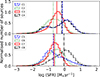 |
Fig. 10. Same as Fig. 9, but for SFR. |
| In the text | |
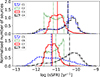 |
Fig. 11. Same as Fig. 9, but for sSFR. |
| In the text | |
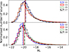 |
Fig. 12. Same as Fig. 9, but for the absolute magnitude in the r band. |
| In the text | |
|
Fig. 13. Comparison of morphological classification of green valley samples for every criterion ranging from C1, C3, C5, and C7 for optically selected sample (top panel) and C2, C4, C6, and C8 for UV-selected sample (bottom panel). The morphological types are from the Galaxy Zoo survey. The blue solid line, red dotted line, and the black dash-dotted line represent spiral, elliptical, and uncertain (unclassified) galaxies, respectively. |
| In the text | |
|
Fig. 14. Distribution of spectroscopic types for green valley galaxies selected using different optical (top) and UV (bottom) criteria. We present the star-forming galaxies (blue solid line), composite galaxies (green dotted line), Seyfert 2 (red dash-dotted line), and LINERs (black dashed line). |
| In the text | |
|
Fig. 15. Mg-Mr (top panel) and MNUV-Mr (bottom panel) colour distributions before (red histograms) and after (blue semi-filled histograms) the extinction correction. The green valley region defined in Sections 3.1.1 and 3.1.2 is represented by two vertical black-dashed lines. |
| In the text | |
|
Fig. 16. Colour-colour criterion, with the possibility of green valley selection using either the g − r (green dot-dashed lines) or the NUV − r (black dashed lines) colours. |
| In the text | |
|
Fig. 17. NUV − r vs. sSFR relation, with the green valley selected with either the sSFR criterion (green dash-dotted lines), NUV − r criterion (black dashed lines), or mixed criteria (blue solid lines). |
| In the text | |
Current usage metrics show cumulative count of Article Views (full-text article views including HTML views, PDF and ePub downloads, according to the available data) and Abstracts Views on Vision4Press platform.
Data correspond to usage on the plateform after 2015. The current usage metrics is available 48-96 hours after online publication and is updated daily on week days.
Initial download of the metrics may take a while.