| Issue |
A&A
Volume 706, February 2026
|
|
|---|---|---|
| Article Number | A325 | |
| Number of page(s) | 17 | |
| Section | Astrophysical processes | |
| DOI | https://doi.org/10.1051/0004-6361/202555617 | |
| Published online | 17 February 2026 | |
Moonlit sky polarization patterns from Cerro Paranal
1
Department of Physics and CENTRA- Center for Astrophysics and Gravitation, Instituto Superior Técnico, University of Lisbon Lisbon, Portugal
2
Instituto de Astrofísica e Ciências do Espaço, Faculdade de Ciências, Universidade de Lisboa, Ed. C8 Campo Grande 1749-016 Lisbon, Portugal
3
European Southern Observatory Alonso de Córdova 3107 Casilla 19 Santiago, Chile
4
Instituto de Astrofísica e Ciências do Espaço, Universidade do Porto, CAUP Rua das Estrelas Porto 4150-762, Portugal
5
Millennium Institute of Astrophysics MAS, Nuncio Monsenor Sotero Sanz 100 Off. 104 Providencia Santiago, Chile
6
Gemini Observatory/NSF’s NOIRLab Casilla 603 La Serena, Chile
7
Department of Applied Physics, School of Engineering, University of Cádiz Campus of Puerto Real E-11519 Cádiz, Spain
★ Corresponding author: This email address is being protected from spambots. You need JavaScript enabled to view it.
Received:
21
May
2025
Accepted:
30
December
2025
Abstract
We investigated the polarization patterns from the moonlit sky as observed from the European Southern Observatory at Cerro Paranal. The moonlit sky background can be significant in astronomical observations and thus be a source of contamination in polarimetric studies. Based on sky observations during full Moon with FORS2 in imaging polarimetric mode, we measured the polarization degree and intensity at different wavelengths and scattering angles from the Moon, and we compared them to theoretical and phenomenological single- and multiple-scattering models. Single-scattering Rayleigh models are able to reproduce the wavelength dependence of the polarization as long as strong depolarization factors that increase with wavelength are introduced. Intensity data, however, require the inclusion of single Mie scattering from larger aerosol particles. The best models that simultaneously fit polarization and intensity data are a combination of the two single-scattering processes, Rayleigh and Mie, plus an unpolarized multiple-scattering component. Both Mie and multiple scattering become more dominant at longer wavelengths. Other factors such as cloud depolarization and the sunlight contribution at twilight were also investigated. The present study underscores the importance of accounting for moonlight scattering to enhance the accuracy of polarimetric observations of astronomical targets.
Key words: polarization / scattering
© The Authors 2026
 Open Access article, published by EDP Sciences, under the terms of the Creative Commons Attribution License (https://creativecommons.org/licenses/by/4.0), which permits unrestricted use, distribution, and reproduction in any medium, provided the original work is properly cited.
This article is published in open access under the Subscribe to Open model. This email address is being protected from spambots. You need JavaScript enabled to view it. to support open access publication.
1. Introduction
The study of polarized light has been crucial in the progress of astronomy. Unique physical properties of astronomical objects can be deduced by analyzing polarized light that reaches the observer. It complements intensity-based methods such as photometry and spectroscopy. For example, optical linear polarimetry has helped consolidate the unification model of active galactic nuclei (Antonucci & Miller 1985), it reveals asymmetries of the ejecta in supernova explosions (e.g., Leonard et al. 2001), the magnetic field structure in galaxies (e.g., Scarrott et al. 1991), dust characteristics in galaxies (Rino-Silvestre et al. 2025), and the composition and geometry of kilonovae (e.g., Bulla et al. 2019).
Polarimetric observations from ground-based telescopes present various challenges. In particular, the scattering of moonlight in Earth’s atmosphere generates polarization patterns that can contaminate polarimetric measurements of astronomical targets. Light polarization by atmospheric scattering has been studied extensively throughout the years. It depends on various factors, such as the scattering angle between the incident moonlight and the atmospheric particles and the atmospheric conditions at different observatory locations.
The Rayleigh model has endured in the scientific community as a good approximation of the daytime sky polarization due to scattering of sunlight in the atmosphere (Chandrasekhar 1960; Coulson 1988; Liou 2002). This theory has been foundational for several studies and advances, such as navigation methods based on polarized light (Liu et al. 2020) and the analysis of exoplanet atmospheres (Madhusudhan & Burrows 2012; Berdyugina et al. 2011). Similarly, Gál et al. (2001) have shown that the patterns of the degree and angle of polarization from the Moon at night are equivalent to the daylight patterns from the Sun. The Rayleigh model predicts maximum polarization at 90º from the Moon at night and two neutral points of zero polarization at the Moon and anti-Moon position. Nonetheless, changes in the relative abundances of atmospheric particles such as air molecules, aerosols, and dust can result in the observation of four neutral points instead (Horváth et al. 2002) due to increased multiple-scattering (MS) processes (Berry et al. 2004; Wang et al. 2016; Harrington et al. 2017). This strongly depends on the atmospheric conditions of the observing site.
This work is devoted to studying the polarization patterns in the moonlit sky and atmospheric scattering processes from the facilities of the European Southern Observatory (ESO) at Cerro Paranal in Chile. The scattered moonlight intensity at Paranal has been studied in detail (Patat et al. 2011; Jones et al. 2019, 2013) but not its polarization. We used existing analytical and empirical models of single-scattering (SS) and MS (Sect. 2) together with observations of the night sky during full Moon from Paranal (Sect. 3), and compared them (Sect. 4) to obtain the best models and parameters that describe these patterns. In Sect. 5 we discuss the implications of our results for the composition of the atmosphere and the prediction of moonlit sky polarization contamination in astronomical polarimetric observations from Paranal.
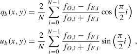
2. Sky model
In this section we present the different components of the sky model used to fit our polarimetric data from Paranal (see Sect. 3). Earth’s atmosphere is composed of particles with which the moonlight of different wavelengths interacts through scattering and absorption generating the intensity and polarimetry patterns in the sky. The atmospheric transmission curve, shown in Fig. 1 of Patat et al. (2011), is characterized by the optical extinction components: Rayleigh scattering by air molecules, Mie scattering by aerosols, and molecular absorption (O2, O3, and H2O). We closely followed the model developed for the optical intensity (Jones et al. 2013, 2019), adapting it here to optical polarimetry.
Figure 1 represents the celestial sphere, where the observer (O) is at the center and the zenith for the observer (ZO) is in the top. θ is the altitude angle from the positive z-axis, and ϕ is the azimuth angle measured from the positive x-axis in the clockwise direction. The target that is being observed (T) and the projected Moon position on the sphere (M) form the scattering angle γ, determined as
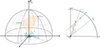 |
Fig. 1. Left: Representation scheme for the scattering geometry in Earth’s atmosphere. Right: Schematic description of the scattering process assuming that the moonlight enters the atmosphere in parallel beams. |
 (1)
(1)
The leading scattering process in the atmosphere is SS, in which the light beam only interacts with the atmosphere once during its entire path to the observer. A light wave enters the atmosphere through M, crosses the path to a scattering point (S), in an arbitrary point on the line between the target and the observer. After interacting with the atmosphere, the photon is scattered into the line of sight toward the observer. Multiple scattering, on the other hand, represents only a few percent of the scattering (Jones et al. 2013) and it occurs when the light interacts several times in the atmosphere before reaching the observer.
The atmosphere contains different types of particles produced by various natural and human-induced processes. The interactions between the light and these atmospheric particles are determined by the interplay between the wavelength of light and the particle size. The latter is generally described by the size parameter x = 2πa/λ, where λ is the wavelength of the incident radiation and a is the typical radius of the particle. Rayleigh scattering occurs for small particles at x < < 1 (typically air molecules including nitrogen, oxygen, and argon), whereas for larger particles (like aerosols) Mie scattering enters into play1.
In the following sections, we review the different scattering mechanisms at play in the atmosphere. We start with some basic concepts including the incident moonlight (Sect. 2.1), the Stokes formalism and scattering matrix (Sect. 2.2), Rayleigh scattering (Sect. 2.4), Mie scattering (Sect. 2.6), and MS (Sect. 2.7).
2.1. Moonlight
The incident moonlight is sunlight reflected at the surface of the Moon. The solar intensity spectrum has been extensively studied (e.g., Colina et al. 1996) while its polarization spectrum – sometimes called the “second solar spectrum” – shows up to a ∼1% continuum polarization (Stenflo & Keller 1997; Stenflo et al. 2000; Stenflo 2005; Gandorfer 2000, 2002). The reflection of the sunlight at the lunar surface can lead to polarization that depends on the lunar phase reaching up to 30% at the Sun’s angular distance of 90º–100º from the Moon (around first and third quarters) and decreasing to zero at 180º or full moon (Kohan 1962; Dollfus & Bowell 1971; Wolff 1975). As our observations were taken during full moon, we assume in the following an unpolarized incoming moonlight spectrum as a first approximation.
2.2. Stokes formalism and radiative transfer
In unpolarized radiation, sometimes referred to as natural light, one deals with an incoherent superposition of electromagnetic waves, meaning all orientations of the electric field vectors are equally probable. A convenient method for describing the polarization transformations of radiation due to scattering and other processes is through the Stokes parameters (Stokes 1851).
The Stokes vector S quantifies light polarization via four parameters (each a vector element): I, Q, U, and V. In this formalism, I represents the total intensity. Q and U represent the linearly polarized intensity; more specifically, Q quantifies a difference in the electric field in the x and y reference frame (the wave propagates in the z-direction and north usually indicates the positive x-axis), and the parameter U quantifies the difference between the two diagonal components (at angles of 45° and 135° counted from the positive x axis). V refers to circularly polarized radiation.
In the absence of additional light sources, the radiation transfer equation describing changes in the radiation vector, S, due to its interaction with the medium can be written as (Steinacker et al. 2013)
 (2)
(2)
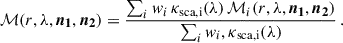
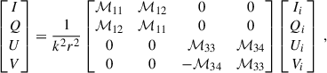
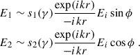
The left-hand side is the change of the radiation over an infinitesimal part of its path (dr). The first term of the right-hand side is the loss of energy due to extinction, and the second term represents the scattering component into the line of sight. The variable δ(r) is the mass density of the medium, κsca is he scattering coefficient, and κext is the mass extinction coefficient, which includes absorption and scattering off the line of sight: κext = κabs + κsca. The scattering matrix (ℳ), or phase matrix, is the Müller 4 × 4 matrix describing the changes of the Stokes vector when radiation is scattered from an initial propagation direction (n1) to a new direction (n2).
An incident Stokes vector Si = (Ii, Qi, Ui, Vi) entering at the Moon position (M) in the celestial sphere gets extincted along its path r1 to the observing target (T) by a factor of exp(−τ1) with
 (3)
(3)
In the case of SS, the solution to Eq. 2 is given by
 (4)
(4)
with τ2 indicating the extinction from S to the observer at position O along the path r2. In the case of sunlit or moonlit sky observations, the only predominant contribution is that from scattering, so the Ssca(λ) in Eq. (4) represents the observed Stokes vector reaching the observer.
It is important to note that in a dust mixture, both the individual coefficients and Müller matrices of each species, i, can be taken into account with their relative contributions wi in Eqs. (2) and (4) (Wolf 2003) as follows:
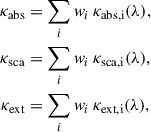 (5)
(5)
and
 (6)
(6)
In the following sections we consider the different types of dust scattering processes contributing to Eq. (4).
2.3. Scattering and Müller matrix
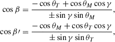
The SS matrix, ℳ, which depends on the initial and final directions of light propagation, n1 and n2, respectively, can also be described via the scattering angle (γ) and two 4 × 4 rotation matrices (rotation in the Q-U plane), R (Liou 2002):
 (7)
(7)
Here β and β′ are rotation angles that relate the meridian and scattering planes:
 (8)
(8)
where the plus sign is used when π < ϕT − ϕM < 2π and the minus sign when 0 < ϕT − ϕM < π.
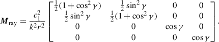
The Müller matrix ℳ describing the scattering of light is composed of 16 independent elements, but the spherical assumptions of the particles reduce this number to four, as described in, for example, Bohren & Huffman 1998 and Narasimhan & Nayar 2003:
 (9)
(9)
where r is the distance from the observer to the scattering element and k is the wave number in the medium related to the angular frequency (ω) and the complex index of refraction (m) of the spherical particle: k = ωm/c. To express the elements of the scattering phase matrix, we used the complex scattering amplitudes s1(m, x, γ) and s2(m, x, γ), which relate to the incoming electric field components as
 (10)
(10)
The subscripts 1 and 2 correspond to two orthogonal orientations that are both perpendicular to the direction of propagation of the incoming wave. The scattering phase matrix elements for a single sphere are then given by
![Mathematical equation: $$ \begin{aligned} \mathcal{M} _{11}&= \frac{1}{2}\left[ s_{1}s_{1}^{*}+s_{2}s_{2}^{*} \right]\\ \mathcal{M} _{12}&= \frac{1}{2}\left[ s_{2}s_{2}^{*}-s_{1}s_{1}^{*} \right]\\ \mathcal{M} _{33}&= \frac{1}{2}\left[ s_{2}s_{1}^{*}+s_{1}s_{2}^{*} \right]\\ \mathcal{M} _{34}&= \frac{-i}{2}\left[ s_{1}s_{2}^{*}-s_{2}s_{1}^{*} \right]. \end{aligned} $$](/articles/aa/full_html/2026/02/aa55617-25/aa55617-25-eq11.gif)
If the incident light is unpolarized, Si = (Ii, 0, 0, 0), and neglecting for now the extinction, then the scattered light has the following components:
 (11)
(11)
or including rotations (Eq. 7):
 (12)
(12)
with the intensity in either case given by
 (13)
(13)
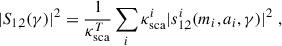
the normalized degree of polarization (DoP), 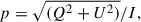 by
by
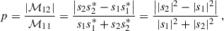 (14)
(14)
and the polarization angle (AoP), χ = 1/2arctan(U/Q), by
 (15)
(15)
For multiple particles, i, with different properties, the individual Müller matrices can be summed (see Eq. (6)), and in the SS case the total squared moduli of the scattering amplitudes S1 and S2 are the sum of the amplitudes of each individual spherical particle, s1i and s2i, taking into account its scattering coefficients (Liou 2002):
 (16)
(16)
with κscaT = ∑iκscai. In the case of a set of particles in the atmosphere with a distribution of sizes, the scattering amplitudes can be integrated over the number density, n(a) (particles per unit volume) with a size parameter between a and a + da:
 (17)
(17)
with κscaT = ∫κsca(a)n(a)da. From these new total scattering amplitudes it is possible to obtain the intensity and the polarization degree as given by Eqs. (13) and (14).
2.4. Rayleigh scattering
Rayleigh scattering (Rayleigh 1871), also referred to Rayleigh-Gans theory, is the main explanation behind phenomena like the blue sky and the red sunrise and sunset. Originally developed for the Sun at daylight, the effects are analogous for the Moon at night. Molecules in the air (mainly nitrogen, oxygen, and argon), assumed spherical with radii a much smaller than the wavelength of the incident radiation (x ≪ 1), scatter preferentially light of smaller wavelengths, i.e., blue light. Such particles represent the majority of particles in the atmosphere and it is therefore the most probable type of scattering. The model assumes that the particles are identical and exist in an isotropic atmosphere. For Rayleigh scattering, the amplitudes are given by (Bohren & Huffman 1998):
 (18)
(18)
such that the following phase matrix can be used:
For unpolarized incoming light (see Eq. (11)), the scattered intensity for Rayleigh has a dependence on the distance (r−2) and on the wavelength (λ−4) –provided that the refractive index (m) does not depend (or only slightly depends) on wavelength:
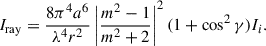 (19)
(19)
The normalized DoP or fraction of polarized light (see Eq. 14) depends only on the scattering angle:
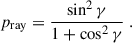 (20)
(20)
Rayleigh theory predicts therefore that in the forward and backward directions the scattered light remains unpolarized while at 90 degrees it is fully polarized; in other directions the light is partially polarized (see the upper-left panel of Fig. 2). No polarization-wavelength dependence is expected from pure Rayleigh scattering.
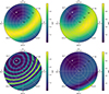 |
Fig. 2. Simulation of sky polarization degree at Paranal on 26 January 2021, according to the single Rayleigh scattering model (upper left), the MS model (upper right) with L = 0.3 or a neutral point angular distance of 67°, and the Mie scattering model of a single-size particle of radius 0.9 μm (lower left) and a log-normal size distribution (lower right). The polarization degree is color-coded, and the Moon’s position is shown as a white circle. |
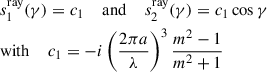
2.5. Anisotropic Rayleigh scattering
The Rayleigh scattering model presented in the previous section assumes only spherical particles, a presumption that breaks down for O2 for example, since it is diatomic and slightly anisotropic. An effective way to include anisotropic particles lies in adding the depolarization factor, δ, to the Rayleigh scattering model (Chandrasekhar 1960; Hansen & Travis 1974), such that the anisotropic amplitudes,  , are
, are
 (21)
(21)
with Δ = (1 − δ)/(1 + δ/2), and the DoP is given by
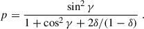 (22)
(22)
The depolarization factor δ is equal or smaller than 0.5. For air, experiments indicate a value of 0.03–0.04 for the depolarization factor (Hansen & Travis 1974).
In the end, Rayleigh scattering is just a limiting case for infinitesimally small particles of the broader Mie framework. Larger particles in the atmosphere, such as aerosols, must be treated with Mie scattering as we do in the next section.
2.6. Mie scattering
Mie scattering, also known as Lorenz-Mie scattering, is a theory derived independently by Mie (1908), assuming that the scattering particle is a homogeneous sphere with a larger size than or equal to the wavelength of the incident ray, i.e., with x ≥ 1. This type of scattering is more probable for aerosols and cloud particles. As a consequence, clouds and non-absorbing aerosols in the atmosphere (like fog effects) generally appear white. The Mie scattering amplitudes are given by (e.g., Liou 2002)
 (23)
(23)
where
 (24)
(24)
and Pn(cos γ) is the Legendre polynomial of order n. The coefficients an and bn are given by
 (25)
(25)
with ψn(q) and ζn(q) being quantities related to the Bessel functions Jn(q) and Hn(q) of the first and second kind, respectively:
 (26)
(26)
The polarization degree for Mie scattering can be calculated using the scattering amplitudes (Eq. (23)) in Eq. (14). The resulting pattern depends not only on the scattering angle but also on the size parameter, i.e., the relation between the radius of the spherical particle and the wavelength.
However, in reality the aerosols of the atmosphere come in several types and follow a log-normal size distribution (Williams & Warneck 2012). The six species of tropospheric and stratospheric aerosols considered in Jones et al. (2019) are shown in Table 1. With a log-normal size distribution of the form
 (27)
(27)
– the characteristic number density (ni), mean radius (ai), and the size distribution (si) per species i are provided in Table 1 – we can use Eq. (17) to model their scattered amplitude as the integral of each individual particle s1, 2i from Eq. (23):
 (28)
(28)
Aerosol modes from Williams & Warneck (2012).
Each species may also have a different refractive index, mi. Examples of Mie scattering for large particles that are identical in size (a = 0.9 μm – tropospheric coarse) and that follow a size distribution in accordance with Eq. (27) are shown in the bottom-left and bottom-right panels of Fig. 2, respectively.
The total Mie SS phase amplitudes from all integrated species are the sum of its six constituents (the relative weights already being determined by their density):
 (29)
(29)
Finally, in order to consider all SS events, including Rayleigh and Mie scattering, the total amplitudes are given by
 (30)
(30)
which can be in turn used to calculate the intensity and polarization degree via Eqs. (13) and (14). The relative weights of each component sum to one, i.e., wray + wmie = 1. For the single size Mie scattering we used the MIEPYTHON software (Prahl 2023)2, and for the log-normal distributed Mie scattering we implemented a PYTHON version of the IDL code developed by G. Thomas3.
2.7. Multiple scattering
The scattering in our atmosphere as seen from Paranal has only a few percent contribution from MS effects, as shown in Jones et al. (2013). Doing a full physical treatment of MS is very difficult. Here we experimented with two approaches: (1) a simple phenomenological model of the polarization pattern originating from MS; and (2) the assumption that an additional component of light from MS is non-polarized.
2.7.1. Phenomenological multiple-scattering polarization
Multiple scattering in the atmosphere has been supported by observations that often show the existence of more neutral polarization points (David 1847; Horváth et al. 2002) than what the single Rayleigh scattering predicts. The four predicted neutral points are located close to the Moon and anti-Moon positions (but not coincident with them), and they can be modeled with radiative transfer assuming MS effects (Chandrasekhar 1950; Chandrasekhar & Elbert 1954). The Berry singularity theory (Berry et al. 2004) provides a simple alternative phenomenological description of the sky polarization pattern with four neutral points that is consistent with both observations and radiative transfer calculations. Here, the polarization can be represented by a complex Stokes parameter:
 (31)
(31)
Then the DoP will be given by pMS = |ω(ξ)| and the polarization direction or the polarization angle is given by γ(ξ). With this description the four neutral points known as Brewster and Babinet points (close the Moon) and Arago and second Brewster points (close to the anti-Moon) are described by the points ξ+, ξ−,  , and
, and  , respectively. To guarantee that the DoP is antipodally invariant, it is imposed that
 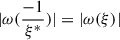 , meaning the function ω(ξ) becomes
 (32)
(32)
with
 (33)
(33)
where x′M = xM/(1 − zM) and y′M = yM/(1 − zM). xM, yM and zM are the coordinates of the Moon, ϕM is the azimuth of the Moon and L is a parameter that is used to describe the degeneration of the two singularities of w(ξ). The angular separation between the two singularities is given by δ = 4arctan(L) (Wang et al. 2016). We used a normalization parameter, A, that multiplies w(ξ) and sets the maximum DoP. In this phenomenological model the sky pattern for the DoP results in the upper-right panel of Fig. 2. However, it does not provide the scattering amplitudes and it is then difficult to combine with other mechanisms. Here we fit it individually to our data to see if it is the leading process in the atmosphere for our observations.
2.7.2. Multiple-scattering intensity
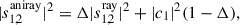
For the intensity contribution from MS, we used the results of Jones et al. (2013), which give a correction factor f(λ, γ) for the SS flux to account for the MS: Itot = ISSf(λ, γ). If we combine this intensity with the polarization pattern predicted by the MS phenomenological model, we can posit the following scattering amplitudes that ensure both the polarization of Berry et al. (2004) and the intensity of Jones et al. (2013):
![Mathematical equation: $$ \begin{aligned} \begin{aligned} |S_1^{\mathrm{MS} }|^2 = \frac{1}{2}\left[|S_1^{\mathrm{SS} }|^2+|S_2^{\mathrm{SS} }|^2\right]\left(f(\lambda ,\gamma )-1\right)\,[1-\omega (\xi )]\,\,\\ |S_2^{\mathrm{MS} }|^2 = \frac{1}{2}\left[|S_1^{\mathrm{SS} }|^2+|S_2^{\mathrm{SS} }|^2\right]\left(f(\lambda ,\gamma )-1\right)\,[1+\omega (\xi )]\,, \end{aligned} \end{aligned} $$](/articles/aa/full_html/2026/02/aa55617-25/aa55617-25-eq41.gif) (34)
(34)
where ω(ξ) is given by Eq. (32). In general, higher-order scattering leads to increased depolarization because of the growing randomness in the direction of scattering of the light. If ω = 0, MS is unpolarized, which means no preferential orientation of the electric field, and the scattering amplitudes would be equal: S1MS = S2MS. The polarization contribution from MS will thus be null, pMS = 0 but not the intensity, IMS = |S1MS|2.
2.8. Total scattering
When we consider all scattering processes – single Rayleigh and Mie scattering, MS, and the extinction factors – we can rewrite the total polarization degree and intensity as
 (35)
(35)
 (36)
(36)
with
 (37)
(37)
and  given by Eq. (30); the weights of each process, w, are free parameters. For simplification in the fits performed in this study, we concentrated on the dependence on wavelength, particle size, and refractive index and assumed that the integrations of path are mostly absorbed by a general constant, I, left free in the fit.
3. Data acquisition
In this section we present the strategy to observe the moonlit sky with the imaging polarimetric mode (IPOL) of the Focal Reducer and low dispersion Spectrograph (FORS2) at the Very Large Telescope (VLT) in Paranal, as well as the data acquisition and reductions we performed.
3.1. Observational strategy
To test the different atmospheric models presented in the previous section, we took polarimetric observations in BVRI filters of fourteen blank fields during the full-moon nights of 25 and 26 January 2021 using FORS2 at VLT through program 106.21L9. Blank fields refer to fields of view devoid of bright sources and are generally used as flat fields for calibrations. Since the polarization pattern for different models changes mostly with scattering angle (see Fig. 2), we tried to cover a wide range of distances from the Moon including also targets close to the Moon to test for neutral points.
Our observations are summarized in Fig. 3, where the field locations are shown in blue, and the Moon positions during the night are represented in black with matching symbols with the field at the time of its observation. We aimed to measure the illuminated sky and therefore the exposure times were calculated based on the number of counts (> 30 k on average per frame), so fields farther from the Moon had longer integration times. The average exposure times per half-wave plate (HWP) angle of all our observed fields are 198, 94, 63, and 63 seconds for B, V, R, and I, respectively.
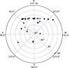 |
Fig. 3. Summary of observations as seen from an observer at Cerro Paranal on two consecutive nights. The zenith is at the center, and the blank fields in the sky (our targets) at the time of observation are shown with blue markers. The corresponding Moon position at the time of observation of each target is shown in black with the same symbol shape. |
On the first night of observations, the weather started with thin cirrus and windy, it evolved to higher seeing values until getting cloudy with thick cirrus and temporarily closing the dome. On the second day of observations, the observing conditions were optimal. Measurements were taken until close to twilight, when the Sun started influencing the polarization pattern. Due to different observation conditions, the data were divided into three different groups: (a) clear data, (b) cloudy data, and (c) twilight data. The median seeing of all our observations was 0.87”. We note that these observations can also help us measure the stability of the FORS2 spatial instrumental corrections found in González-Gaitán et al. (2020), as will be presented elsewhere.
3.2. Polarimetric measurements
The FORS2 instrument is a dual-beam polarimeter, in which one measures simultaneously the intensity of the two perpendicular polarization components of the incident light beam. The beam is divided in two by a Wollaston prism, whereas the rotatable HWP, placed before the Wollaston prism, allows measurement at different position angles θi. With the HWP at a position i, two intensities designed as ordinary (fO, i) and extraordinary (fE, i) beams are derived. We took here four HWP angles for every field: 0°, 22.5, 45°, and 67.5°.
Since the fields are evenly illuminated and the polarization is not expected to change substantially in the 7′field of view, all pixels can be used to obtain the polarization of the field. As in González-Gaitán et al. (2020), we binned the fluxes in 30 × 30 pixels in x and y by taking the median and the standard deviation as the characteristic value and uncertainty of each box.
The Stokes parameters can then be computed from these set of binned beams, through either the double-difference or double-ratio methods (Bagnulo et al. 2009). Note that we assumed only linear polarization and therefore V = 0. The normalized binned parameters are designated as qb and ub, and correspond to the parameter divided by the total intensity: qb ≡ Qb/Ib and ub ≡ Ub/Ib, respectively. In the double-difference method,
 (38)
(38)
where N = 4 is the total number of HWP position angles. To obtain a final value for the entire field, we took the median and standard deviation of all binned qb, ub values:
 (39)
(39)
There is a spurious spatial instrumental polarization pattern that is axisymmetric in both q and u (González-Gaitán et al. 2020) and thus in principle removed with the median. However, we verified that the values were consistent when doing first an instrumental field correction to the binned qb, ub values before taking the median (Eq. (39)).
The polarization degree and polarization angle are then given by:
 (40)
(40)
The errors associated with the degree and angle of polarization can be obtained by propagating the uncertainties as in the following relation:
 (41)
(41)
where δq and δu are the uncertainties associated with q and u. The full list of obtained quantities is presented in Appendix F.
4. Results
In this section we compare the theoretical scattering predictions with our FORS2-IPOL observations. The observations were done during two nights near full Moon and the Moon’s phase variation during those two nights of observation is assumed to be irrelevant in the models. We used not only the polarization degree observations but also the intensity measurements that will help disentangle the various models. The polarization angle is largely independent of the atmospheric models (see Eq. (15)) and is shown in Appendix A. We focus here on results obtained from data acquired in clear sky conditions, and refer the reader to Appendix B for the atmospheric corrections and Appendix C for twilight data.
Our fits are Levenberg-Marquardt minimizations through the LMFIT package4 (Newville et al. 2016) followed by posterior sampling with a Markov chain Monte Carlo (MCMC; see Appendix D) with the EMCEE package (Foreman-Mackey et al. 2013). To compare models with a different number of free parameters, we made use of the Bayesian information criterion (BIC), a diagnostic of the quality of the fit that penalizes a higher number of free parameters in the model. Lower values indicate model preference, especially when the difference between two models, ΔBIC, is larger than 10.
Polarization fit results.
4.1. Rayleigh scattering
Here we fit the Rayleigh scattering model first to the polarization degree, then the intensity, and finally to both polarization and intensity simultaneously.
4.1.1. Polarization fits:
As can be seen in the left panel of Fig. 4, the polarization degree follows a scattering angle pattern very similar to the Rayleigh phase function peaking near 90° and close to zero at forward and backward directions (see Eq. (20)). However, pure single Rayleigh scattering predicts 100% peak polarization at all wavelengths, which is not seen here. In fact, in order to fit a Rayleigh model to the data, we needed to assume anisotropic grains that strongly depolarize the light with a wavelength-dependent factor δ(λ), as in Eq. (22), the only free parameter in each fit. The fitted models for each band are represented with dashed lines in the left panel and the parameters and BIC values are shown in Table 2. Clearly, the depolarization is stronger as we go to longer wavelengths increasing from δ = 0.03 to 0.12 following a power law (see Appendix E). The bluer wavelengths agree with measured atmospheric values (e.g., 0.02 for H2, 0.03 for air and N2, 0.06 for O2, and 0.09 for CO2; see, e.g., Penndorf 1957), whereas the reddest bands show clear signals of increased depolarization, probably from nonspherical particles (such as ice crystals, snowflakes, or dust particles) or from enhanced MS (Sassen 1991). Other effects beyond pure Rayleigh scattering become more dominant with wavelength as indicated by the growing depolarization. The decreasing BIC values with wavelength confirm that models with deviations from pure Rayleigh due to depolarization are preferred.
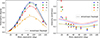 |
Fig. 4. Polarization degree (left) and intensity in arbitrary units (right) versus scattering angle from the Moon. Points are observations in different bands (uncertainties are smaller than the points: ∼0.001–0.01 for polarization and ∼0.001–0.02 for intensity), and lines are individual fits to each band for anisotropic Rayleigh scattering. |
4.1.2. Intensity fits:
As can be seen in the right panel of Fig. 4, the intensity grows strongly at small scattering angles, a pattern that is more reminiscent of the Mie scattering phase function and inconsistent with Rayleigh scattering. Doing individual fits to each band’s intensity, we obtain the dashed lines shown in the right panel, which clearly under-predict the intensity at small angles and result in high BIC values, as shown in Table 3. We note that the intensity is normalized by a global factor that preserves its wavelength and scattering angle dependence. The Rayleigh model thus has an additional free normalization parameter for the intensity for a total of two parameters (δ and I). We note that the depolarization factor does not have an effect on the intensity.
Intensity fit results.
4.1.3. Polarization and intensity fits:
A simultaneous fit to both the polarization and intensity data for each band results in the dotted lines shown in Figs. 7 and 8. These are isotropic Rayleigh fits with no depolarization factor and thus peaking at 100% polarization degree.
We conclude that Rayleigh scattering alone is unable to reproduce the observations.
4.2. Mie scattering
We now show the results of pure Mie scattering fitted to the data: polarization, intensity and joint polarization-intensity fits. We concentrated on Mie scattering with four aerosol species (the first four in Table 1) and fixed their respective fractions to the values obtained by Jones et al. (2013, 2019). We assumed that all species have the same refractive index (without the imaginary component, i.e., the absorption coefficient). These constraints are relaxed in Sect. 4.5.
4.2.1. Polarization fits:
For Mie scattering we obtain the polarization fits shown in the left panel of Fig. 5. The fits are much worse than for Rayleigh scattering with a peak in polarization degree at higher angles than the observed ∼90°. The worse fits are also seen in much higher BIC values (ΔBIC> 15). The obtained refractive index ranges between 1.4 and 1.5, in agreement with measured values (Elterman 1966; Yue et al. 1994); however in B, the refractive index is too high, m = 1.80 ± 0.09, indicating that Mie is even less compatible at these wavelengths. This is expected as aerosol particles responsible for Mie scattering are larger with higher cross sections at longer wavelengths of light. The fits are indeed also better at increasing wavelengths according to the BIC values.
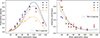 |
Fig. 5. Polarization degree (left) and normalized intensity (right) versus scattering angle from the Moon. Points are observations in different bands (uncertainties are smaller than the points), and lines are individual fits to each band for Mie scattering with four species and a single refractive index. |
4.2.2. Intensity fits:
Regarding the intensity fits, the Mie scattering model is capable of reproducing the sharp increase at small scattering angles providing much better fits than pure Rayleigh scattering (also seen in ΔBIC < − 10 of Table 3). However, at larger scattering angles, the Mie models underestimate the observed intensities. The fitted refractive indices are rather large (m > 1.8), except for the I band, showing that Mie scattering alone cannot reproduce the intensity data. The I-band wavelength is more compatible with observed refractive indices (1.29 ± 0.09) pointing again to a predominance of Mie at longer wavelengths.
4.2.3. Polarization and intensity fits:
In Figs. 7 and 8 and Table 4 we confirm the fits with only polarization and the ones with only intensity data: although Mie scattering provides overall better fits than Rayleigh scattering, a combination of the two processes probably reconciles the shortcomings of both.
Polarization and intensity fit results.
4.3. Multiple scattering
We also fit the phenomenological MS model of Eq. (32) to our observed polarization data, as shown in Fig. 6. In this case the deviation from pure Rayleigh is given by the L parameter, a measure of the distance between the two neutral points (see Sect 2.7.1). We recover SS, i.e., L = 0, for BVR bands. For the I band, however, the value is larger than zero, although within the uncertainties (L = 0.08 ± 0.12). The value L = 0.08 corresponds to an 18° angular distance between neutral points, which is slightly lower than what is found at other observing sites (22°–40°; Horváth et al. 2002). Nonzero L values for the I band confirm that MS is more relevant at longer wavelengths because of the presence of larger atmospheric particles (like aerosols). Similarly as with anisotropic Rayleigh and Mie scattering, the BIC values also reveal better fits at longer wavelengths. We note, however, that to constrain this model better, more data near the neutral points are required.
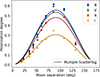 |
Fig. 6. Polarization degree versus scattering angle from the Moon. Points are observations in different bands (uncertainties are smaller than the points), and lines are individual fits to each band for the phenomenological MS model. |
Since our Paranal fits result in insignificant L values, we assumed here that MS does not induce significant polarization but rather only depolarizes the light. As such, hereafter, MS is added as an intensity component without polarization signature (ω = 0 in Eq. (34)).
4.4. Combined scattering processes
We have shown that both main processes of SS, Rayleigh and Mie, are present in the DoP and intensity data taken during full Moon at Paranal. Here we combine the two processes, as in Eq. (30), explore the inclusion of the unpolarized MS effects as in Eq. (37), and fit them to the data.
4.4.1. Polarization fits:
The resulting fits for individual DoP fits are shown in Table 2. We find that the combined models are good representations of the polarization data. This shows that scattering by a set of nonidentical particles results in depolarization – we used a spherical Rayleigh component, i.e., no depolarization factor (Bohren & Huffman 1998). However, the simplicity of the anisotropic Rayleigh scattering still prevails, as seen from the lowest BIC values. Nevertheless, the BIC differences in the RI bands between the Rayleigh-Mie-MS model and pure anisotropic Rayleigh scattering are less than 5. It is interesting to note that the ratio of Rayleigh-to-Mie scattering decreases with wavelength in both combined models, an expected trend (see, e.g., Fig. 1 of Patat et al. 2011). Additionally, the MS weight increases, again showing that Mie and MS scattering from larger particles are increasingly important at longer wavelengths.
4.4.2. Intensity fits:
The intensity fits clearly show that the combined models are preferred according to the BIC (see Table 3). The additional unpolarized MS component is significantly preferred for redder bands as seen in the MS parameter and the decreased BIC values. Similarly to the polarization fits, the Mie and MS components become more important at longer wavelengths.
4.4.3. Polarization and Intensity fits:
Simultaneous fits to intensity and polarization in each band are shown in Table 4 and as solid lines in Figs. 7 and 8. It is evident that these combined processes better explain the data. The joint Rayleigh-Mie-MS scattering is the best of all models by ΔBIC< 30 for all bands. The resulting Mie contribution increases with wavelength, as does the MS component.
We note that models including MS are roughly equivalent to models with anisotropic Rayleigh scattering: they both act as a depolarizer. When both effects are taken into account in the fit, one of the two parameters, the MS fraction or the depolarization factor δ, is consistent with zero, showing that they achieve equivalent results.
4.5. Multiwavelength fits
The models considered in this study, for example Eq. (29), have a wavelength dependence, but refractive indices generally also depend on wavelength. On the other hand, the global ratio of Rayleigh to Mie scattering should be constant if the wavelength dependence is already considered in the models. Similarly, MS, as given in Eq. (34), already has a measured wavelength dependence, f(λ), so its fraction should be a constant. In this section we attempt to simultaneously fit all four photometric bands to the various combined models presented earlier.
By allowing only a single refractive index for all bands, no model is capable of simultaneously reproducing all bands. If we allow the relative fraction of the four Mie aerosol species to be free in the fit, the results are more promising, as shown in Fig. 9 and Table 5. In particular, we find that larger fractions of the tropospheric coarse aerosol is preferred, which is precisely the larger of the four aerosols (a = 0.9 μm) in Table 1. Additionally, a nonzero imaginary part of the refractive index also gives more flexibility to the model increasing the wavelength-dependent extinction.
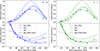 |
Fig. 7. Polarization degree (upper) and normalized intensity (lower) versus scattering angle from the Moon for B (left) and V (right) bands. Points are observations in different bands, and lines are polarization-intensity fits to each band. Error bars are smaller than the data points (∼0.001-0.01 for polarization and ∼0.001-0.02 for intensity). |
We find that mixed models that include anisotropic Rayleigh scattering with large depolarization factors are preferred over regular Rayleigh with MS contributions. However, the predicted depolarization factors are extremely large (δ ∼ 0.5) compensating for the lack of MS component. Allowing for both anisotropic Rayleigh and MS results in fits where the MS fraction is consistent with zero.
Despite the overall match of the models as seen in Fig. 9, the fits to individual bands of previous sections were generally better. Clearly, more flexibility could be attained by having more than a single refractive index for all four species, by having all six aerosol species contributing, or by allowing the refractive index to change with wavelength. However, having only ten data points in each band makes the estimation of so many parameters very difficult. In fact, already some of the parameters are poorly constrained, as seen in Table 5.
Multiwavelength polarization and intensity fit results.
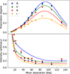 |
Fig. 9. Combined anisotropic Rayleigh + Mie scattering model with four aerosol species (with free relative fractions) and a common complex refractive index fitted to simultaneous polarization (upper) and intensity (lower) multiwavelength data. Errors are smaller than the points. |
5. Conclusions
We have analyzed full Moon observations from Paranal obtained with FORS2-IPOL and compared them to various scattering models. The DoP of the full moonlit sky peaks near a 90° angular separation between the observation target and the Moon, decreasing strongly with wavelength (from 60% in the B band to 30% in the I band). Such a pattern is well fit with simple anisotropic Rayleigh scattering models with depolarization factors that increase with wavelength (from 0.03 to 0.11), suggesting an incremental influence of asphericity and/or MS. The phenomenological framework of Berry et al. (2004) also confirms that MS becomes more dominant at the reddest bands.
The intensity data are inconsistent with pure Rayleigh scattering and clearly require a Mie scattering component from larger aerosol particles. A combined model of Rayleigh and Mie SS plus a MS contribution, as in Jones et al. (2013), is best suited to the individual band fits to both polarization and intensity data. In these fits, the Mie and MS components become more significant at longer wavelengths.
To fit all wavelengths simultaneously, we required higher contributions of large aerosol species and/or a larger extinction (imaginary) part of the refractive index. It is difficult to constrain these parameters with our current dataset.
Future improvements in the fits would allow the different fractions and refractive indices of the six aerosols (Table 1) to vary independently. To achieve this, more data are needed, either from new observations or through a careful inspection of archival FORS2 polarization data of a moonlit sky. Particularly interesting for the angular distance between neutral points from MS is data near the Moon (or anti-Moon) positions, which is scarce given its impracticality in scientific observations.
We stress that if a general physical model that explains all observations is not required and only an estimate or prediction of the polarization pattern is needed, then simple anisotropic Rayleigh scattering provides an excellent description of the polarization. Such a model with depolarization increasing with wavelength (following a power-law dependence) explains full moonlit sky polarization and could be used to correct the background polarization of science targets. It remains to be seen whether the model can explain the data of other nights with different Moon phases as well. In particular, at waning or waxing phases, the polarization of the incoming spectrum reflected off the Moon becomes more important and cannot be neglected, as we did in this study.
Finally, it is worth mentioning that linearly polarized laser radars (lidars) have been successfully used to measure the scattering properties of the atmospheric clouds (Schotland et al. 1971; Sassen 1991). Such experiments could be performed at Paranal to understand the characteristics of the aerosols and improve the modeling.
The atmospheric models presented in this study can be used to correct the polarimetric data of astronomical sources taken on nights with background moonlight in the sky. In particular, simple anisotropic Rayleigh models with wavelength-dependent depolarization factors reproduce the DoP very well (but not the intensity) and can be used as proxies for the moonlit sky polarization.
Acknowledgments
We thank Koraljka Mužić and Evgenij S. Zubko for useful discussions. This work is based on observations collected at the European Southern Observatory under ESO programme 106.21L9. S.G.G. acknowledges support from the ESO Scientific Visitor Programme. A.M.G. acknowledges financial support from grant PID2023-152609OA-I00, funded by the Spanish Ministerio de Ciencia, Innovación y Universidades (MICIU), the Agencia Estatal de Investigación (AEI, 10.13039/501100011033), and the European Union’s European Regional Development Fund (ERDF). The authors thank the Fundação para a Ciência e Tecnologia (FCT) for the financial support to the Center for Astrophysics and Gravitation (CENTRA/IST/ULisboa) through grant No. UID/PRR/00099/2025 (https://doi.org/10.54499/UID/PRR/00099/2025) and grant No. UID/00099/2025 (https://doi.org/10.54499/UID/00099/2025).
References
- Andersson, B. G., Piirola, V., De Buizer, J., et al. 2013, ApJ, 775, 84 [NASA ADS] [CrossRef] [Google Scholar]
- Antonucci, R. R. J., & Miller, J. S. 1985, ApJ, 297, 621 [NASA ADS] [CrossRef] [Google Scholar]
- Bagnulo, S., Landolfi, M., Landstreet, J. D., et al. 2009, PASP, 121, 993 [Google Scholar]
- Berdyugina, S. V., Berdyugin, A. V., Fluri, D. M., & Piirola, V. 2011, ApJ, 728, L6 [NASA ADS] [CrossRef] [Google Scholar]
- Berry, M. V., Dennis, M. R., & Lee, R. L. 2004, New J. Phys., 6, 162 [Google Scholar]
- Bohren, C. F., & Huffman, D. R. 1998, Absorption and Scattering of Light by Small Particles (Wiley) [Google Scholar]
- Bulla, M., Covino, S., Kyutoku, K., et al. 2019, Nat. Astron., 3, 99 [Google Scholar]
- Chandrasekhar, S. 1950, Radiative transfer (Oxford: Clarendon Press) [Google Scholar]
- Chandrasekhar, S. 1960, Radiative transfer (New York: Dover) [Google Scholar]
- Chandrasekhar, S., & Elbert, D. D. 1954, The illumination and polarization of the sunlit sky on Rayleigh scattering [Google Scholar]
- Colina, L., Bohlin, R. C., & Castelli, F. 1996, AJ, 112, 307 [NASA ADS] [CrossRef] [Google Scholar]
- Coulson, K. 1988, Polarization and Intensity of Light in the Atmosphere, Studies in geophysical optics and remote sensing (A. Deepak Pub.) [Google Scholar]
- David, B. 1847, Phil. Mag., 31, 444 [Google Scholar]
- Dollfus, A., & Bowell, E. 1971, A&A, 10, 29 [NASA ADS] [Google Scholar]
- Elterman, L. 1966, Appl. Opt., 5, 1769 [Google Scholar]
- Foreman-Mackey, D., Hogg, D. W., Lang, D., & Goodman, J. 2013, PASP, 125, 306 [Google Scholar]
- Gál, J., Horváth, G., Barta, A., & Wehner, R. 2001, J. Geophys. Res., 106, 22647 [Google Scholar]
- Gandorfer, A. 2000, The Second Solar Spectrum: A high spectral resolution polarimetric survey of scattering polarization at the solar limb in graphical representation. Volume I: 4625 Å to 6995 Å [Google Scholar]
- Gandorfer, A. 2002, The Second Solar Spectrum: A high spectral resolution polarimetric survey of scattering polarization at the solar limb in graphical representation. Volume II: 3910 Å to 4630 Å [Google Scholar]
- González-Gaitán, S., Mourão, A. M., Patat, F., et al. 2020, A&A, 634, A70 [NASA ADS] [CrossRef] [EDP Sciences] [Google Scholar]
- Hansen, J. E., & Travis, L. D. 1974, Space Sci. Rev., 16, 527 [Google Scholar]
- Harrington, D. M., Kuhn, J. R., & Ariste, A. L. 2017, J. Astron. Telescopes Instrum. Syst., 3, 018001 [Google Scholar]
- Horváth, G., Bernáth, B., Suhai, B., Barta, A., & Wehner, R. 2002, JOSA A, 19, 2085 [Google Scholar]
- Jones, A., Noll, S., Kausch, W., Szyszka, C., & Kimeswenger, S. 2013, A&A, 560, A91 [NASA ADS] [CrossRef] [EDP Sciences] [Google Scholar]
- Jones, A., Noll, S., Kausch, W., et al. 2019, A&A, 624, A39 [NASA ADS] [CrossRef] [EDP Sciences] [Google Scholar]
- Kohan, E. K. 1962, in The Moon, eds. Z. Kopal& Z. K. Mikhailov, 14, 453 [Google Scholar]
- Leonard, D. C., Filippenko, A. V., Ardila, D. R., & Brotherton, M. S. 2001, ApJ, 553, 861 [NASA ADS] [CrossRef] [Google Scholar]
- Liou, K.N. 2002, An introduction to atmospheric radiation Vol. 84 (Elsevier), [Google Scholar]
- Liu, B., Fan, Z., & Wang, X. 2020, IEEE Access, 8, 56720 [Google Scholar]
- Madhusudhan, N., & Burrows, A. 2012, ApJ, 747, 25 [NASA ADS] [CrossRef] [Google Scholar]
- Mie, G. 1908, Annalen der Physik, 330, 377 [CrossRef] [Google Scholar]
- Narasimhan, S., & Nayar, S. 2003, IEEE Comput. Soc. Conf. Comput. Vision Pattern Recog., 1, I [Google Scholar]
- Newville, M., Stensitzki, T., Allen, D. B., et al. 2016, Astrophysics Source Code Library [record ascl:1606.014] [Google Scholar]
- Patat, F., Moehler, S., O’Brien, K., et al. 2011, A&A, 527, A91 [NASA ADS] [CrossRef] [EDP Sciences] [Google Scholar]
- Penndorf, R. 1957, J. Opt. Soc. Am., 47, 176 [Google Scholar]
- Prahl, S. 2023, https://doi.org/10.5281/zenodo.7949403 [Google Scholar]
- Rayleigh, L. 1871, Phil. Mag., 41, 274 [Google Scholar]
- Rino-Silvestre, J., González-Gaitán, S., Mourão, A., Duarte, J., & Pereira, B. 2025, A&A, 703, A170 [NASA ADS] [CrossRef] [EDP Sciences] [Google Scholar]
- Sassen, K. 1991, Bull. Am. Meteorol. Soc., 72, 1848 [Google Scholar]
- Scarrott, S. M., Rolph, C. D., Wolstencroft, R. W., & Tadhunter, C. N. 1991, MNRAS, 249, 16P [Google Scholar]
- Schotland, R. M., Sassen, K., & Stone, R. 1971, J. Appl. Meteorol. Climatol., 10, 1011 [Google Scholar]
- Steinacker, J., Baes, M., & Gordon, K. D. 2013, ARA&A, 51, 63 [CrossRef] [Google Scholar]
- Stenflo, J. O. 2005, A&A, 429, 713 [NASA ADS] [CrossRef] [EDP Sciences] [Google Scholar]
- Stenflo, J. O., & Keller, C. U. 1997, A&A, 321, 927 [NASA ADS] [Google Scholar]
- Stenflo, J. O., Keller, C. U., & Gandorfer, A. 2000, A&A, 355, 789 [NASA ADS] [Google Scholar]
- Stokes, G. G. 1851, Trans. Cambridge Philos. Soc., 9, 399 [NASA ADS] [Google Scholar]
- Stuke, S. 2016, Ph.D. Thesis [Google Scholar]
- Wang, X., Gao, J., Fan, Z., & Roberts, N. W. 2016, J. Opt., 18, 065601 [Google Scholar]
- Williams, J., & Warneck, P. 2012, The Atmospheric Chemist Companion [Google Scholar]
- Wolf, S. 2003, ApJ, 582, 859 [NASA ADS] [CrossRef] [Google Scholar]
- Wolff, M. 1975, Appl. Opt., 14, 1395 [NASA ADS] [CrossRef] [Google Scholar]
- Yue, G. K., Poole, L. R., Wang, P. H., & Chiou, E. W. 1994, J. Geophys. Res., 99, 3727 [Google Scholar]
See, e.g., Fig. 5 of Stuke (2016) for a summary of the different wavelengths of the light and particle sizes in the atmosphere.
Appendix A: Polarization angle
We present in Fig. A.1 the measured polarization angle at different angular separations from the Moon in different filters. The stars represent the expected angle obtained from incoming unpolarized light that is scattered in the atmosphere. In such a case, the polarization angle is only dependent on the scattering plane with respect to the incoming light and the observer (see Eqs. 7 and 15), and does not depend on the atmospheric particles nor on the wavelength of the light. The variations seen in the model among different filters arise because of the different times of observation that influence the relative Moon-scattering-observer angles. We roughly confirm here the expected angles, although there are clear discrepancies for certain observations, notably at γ ∼ 35° and γ ∼ 130°.
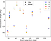 |
Fig. A.1. Observed polarization angle (points) versus moon separation compared to the expected angle (stars) obtained from simple rotations of the scattering plane (Eqs. 7 and 15). |
Appendix B: Atmospheric considerations
Although no specific polarimetric models exist for Paranal, general analytic models include the depolarization effects of the turbidity and optical thickness of the atmosphere based on empirical corrections. In the study of Wang et al. (2016), the stronger depolarization effects near the horizon compared with the zenith are modeled by introducing a horizon correction factor, E, that has a minimum value at the zenith (θ = 0°) and decreases toward the horizon (θ = 90°). So the correction becomes:  , where N is a control parameter used as a free parameter to fit. In addition, they include a correction factor related to the turbulence of the atmosphere. We considered here the "seeing" (S) parameter to be an indicator of the turbulent air flows in the atmosphere. The turbulence generates a gradual depolarization, M(S), that follows an exponential fall off:
  , where the constants k1 and k2 are free parameters used to fit the relationship. Considering these two effects, the corrected polarization degree is described by:
 (B.1)
(B.1)
Using the formalism of Eq. B.1 to correct a pure Rayleigh scattering model, we obtained the fits shown in Fig. B.1. They reveal improvements in the χ2 with respect to pure Rayleigh, yet the BIC values worsen with the increase of free parameters. It is encouraging to see that such empirical corrections can indeed improve the fits. This might be of particular importance with larger, more heterogeneous datasets.
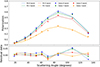 |
Fig. B.1. Fits when taking into account the atmospheric corrections of Eq. B.1 for the single Rayleigh scattering model. |
Appendix C: Twilight data
We analyzed the Sun polarization contribution from twilight data – which corresponds to the Sun being 18° below the horizon or higher. To consider both sources, the Moon and the Sun, their Stokes vectors were added in the Muller calculations, and the albedo was considered to be the sum of each light source contribution.
We assumed pure Rayleigh scattering and a relative light fraction parameter, f, between the two sources. The Sun-Moon model shown in Fig. C.1 fits the data well, including the dip due to twilight. The fit values for the fraction parameter f are shown in Table C.1.
Fit results for parameter f in each band.
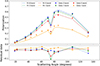 |
Fig. C.1. Fit of the Rayleigh model when taking the polarization with the contribution from the Sun into account. |
Appendix D: MCMC sampling
We show here an example of the MCMC sampling results. In each case, we sampled the parameter space with 132 walkers and 800 iterations with a burn-in of 200 iterations. For a few cases, we extended the sampling to 1200 and burn-in to 600 iterations when the chains had not converged. The priors used are flat for all parameters. In Fig. D.1 we show the corner plot for a Rayleigh-Mie-MS fit to the B band and in Fig. D.2 we show its corresponding fit with 200 realizations from the posterior distribution shown in light blue. We note that in all cases the median values of the posterior distribution are consistent within 1σ with the Levenberg-Marquardt minimization results.
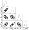 |
Fig. D.1. Corner plot of the four free parameters of an isotropic Rayleigh-Mie-MS model (four Mie species with fixed fractions and unpolarized MS) fitted to the B band: the real refractive index (mr), the intensity normalization parameter (I), the Rayleigh component (R; the Mie M component is given by M = 1 − R), and the MS factor (MS). |
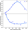 |
Fig. D.2. Rayleigh-Mie-MS fit (blue lines) to B-band polarization data (upper) and intensity data (lower). Uncertainties are smaller than the data points. The dark and light blue lines represent the median and 200 realizations drawn from the posterior distribution of the MCMC, respectively. |
Appendix E: Polarization wavelength dependence
In this section we investigate the wavelength dependence of the polarization data. Since polarization only is modeled very well with only Rayleigh scattering, we studied the obtained depolarization factor, δ(λ), from the anisotropic Rayleigh fits (Eq. 22). Additionally, we also considered a simple constant, A(λ), that multiplies the Rayleigh scattering in each band (Eq. 20). We fit both relations to a power law of the form: p = Bλn + C, as shown in Fig. E.1 and Table E.1. The recovered power laws are in disagreement with previous claims of n = −4 (Andersson et al. 2013). This stems probably from the different combination at various wavelengths of several atmospheric species and scattering processes (single Rayleigh and Mie scattering, and MS).
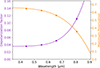 |
Fig. E.1. Wavelength dependence of the depolarization factor, δ, for anisotropic Rayleigh scattering (purple) and a normalization factor, A, multiplying a pure Rayleigh model (uncertainties are smaller than data points). The lines are power-law fits to the data (see Table E.1). |
Parameters of a power-law fit (p = Bλn + C) to δ(λ) and A(λ).
Appendix F: Observational data
Summary of the observational data obtained with the B filter.
We present in Tables F.1, F.2, F.3, and F.4 the BVRI data obtained with FOR2-IPOL. In the table columns, Field refers to the name of the observed region, RA and Dec indicate the right ascension and declination of the field center in degrees,  corresponds to the average universal time during the observation, Exp is the exposure time in seconds, Seeing denotes the atmospheric seeing conditions during the observation in arcseconds, A represents the albedo at the time of observation expressed as a percentage, γ is the scattering angle in degrees, AOP refers to the angle of polarization in degrees, and the DoP is in percentages. All data are presented regardless of the observation conditions. We note that the field CT1 was observed with eight HWP angle positions (see González-Gaitán et al. 2020).
Summary of the observational data obtained with the V filter.
Summary of the observational data obtained with the R filter.
Summary of the observational data obtained with the I filter.
All Tables
All Figures
|
Fig. 1. Left: Representation scheme for the scattering geometry in Earth’s atmosphere. Right: Schematic description of the scattering process assuming that the moonlight enters the atmosphere in parallel beams. |
| In the text | |
|
Fig. 2. Simulation of sky polarization degree at Paranal on 26 January 2021, according to the single Rayleigh scattering model (upper left), the MS model (upper right) with L = 0.3 or a neutral point angular distance of 67°, and the Mie scattering model of a single-size particle of radius 0.9 μm (lower left) and a log-normal size distribution (lower right). The polarization degree is color-coded, and the Moon’s position is shown as a white circle. |
| In the text | |
|
Fig. 3. Summary of observations as seen from an observer at Cerro Paranal on two consecutive nights. The zenith is at the center, and the blank fields in the sky (our targets) at the time of observation are shown with blue markers. The corresponding Moon position at the time of observation of each target is shown in black with the same symbol shape. |
| In the text | |
|
Fig. 4. Polarization degree (left) and intensity in arbitrary units (right) versus scattering angle from the Moon. Points are observations in different bands (uncertainties are smaller than the points: ∼0.001–0.01 for polarization and ∼0.001–0.02 for intensity), and lines are individual fits to each band for anisotropic Rayleigh scattering. |
| In the text | |
|
Fig. 5. Polarization degree (left) and normalized intensity (right) versus scattering angle from the Moon. Points are observations in different bands (uncertainties are smaller than the points), and lines are individual fits to each band for Mie scattering with four species and a single refractive index. |
| In the text | |
|
Fig. 6. Polarization degree versus scattering angle from the Moon. Points are observations in different bands (uncertainties are smaller than the points), and lines are individual fits to each band for the phenomenological MS model. |
| In the text | |
|
Fig. 7. Polarization degree (upper) and normalized intensity (lower) versus scattering angle from the Moon for B (left) and V (right) bands. Points are observations in different bands, and lines are polarization-intensity fits to each band. Error bars are smaller than the data points (∼0.001-0.01 for polarization and ∼0.001-0.02 for intensity). |
| In the text | |
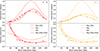 |
Fig. 8. Same as Fig. 7 but for R (left) and I (right) bands. |
| In the text | |
|
Fig. 9. Combined anisotropic Rayleigh + Mie scattering model with four aerosol species (with free relative fractions) and a common complex refractive index fitted to simultaneous polarization (upper) and intensity (lower) multiwavelength data. Errors are smaller than the points. |
| In the text | |
|
Fig. A.1. Observed polarization angle (points) versus moon separation compared to the expected angle (stars) obtained from simple rotations of the scattering plane (Eqs. 7 and 15). |
| In the text | |
|
Fig. B.1. Fits when taking into account the atmospheric corrections of Eq. B.1 for the single Rayleigh scattering model. |
| In the text | |
|
Fig. C.1. Fit of the Rayleigh model when taking the polarization with the contribution from the Sun into account. |
| In the text | |
|
Fig. D.1. Corner plot of the four free parameters of an isotropic Rayleigh-Mie-MS model (four Mie species with fixed fractions and unpolarized MS) fitted to the B band: the real refractive index (mr), the intensity normalization parameter (I), the Rayleigh component (R; the Mie M component is given by M = 1 − R), and the MS factor (MS). |
| In the text | |
|
Fig. D.2. Rayleigh-Mie-MS fit (blue lines) to B-band polarization data (upper) and intensity data (lower). Uncertainties are smaller than the data points. The dark and light blue lines represent the median and 200 realizations drawn from the posterior distribution of the MCMC, respectively. |
| In the text | |
|
Fig. E.1. Wavelength dependence of the depolarization factor, δ, for anisotropic Rayleigh scattering (purple) and a normalization factor, A, multiplying a pure Rayleigh model (uncertainties are smaller than data points). The lines are power-law fits to the data (see Table E.1). |
| In the text | |
Current usage metrics show cumulative count of Article Views (full-text article views including HTML views, PDF and ePub downloads, according to the available data) and Abstracts Views on Vision4Press platform.
Data correspond to usage on the plateform after 2015. The current usage metrics is available 48-96 hours after online publication and is updated daily on week days.
Initial download of the metrics may take a while.