| Issue |
A&A
Volume 706, February 2026
|
|
|---|---|---|
| Article Number | A311 | |
| Number of page(s) | 12 | |
| Section | Astrophysical processes | |
| DOI | https://doi.org/10.1051/0004-6361/202555779 | |
| Published online | 18 February 2026 | |
Non-synchronous rotation in massive binary systems
III. Characterizing five binary systems with fast-rotating OB Stars★
1
Instituto de Astrofísica de La Plata, CONICET–UNLP Paseo del Bosque s/n B1900FWA La Plata, Argentina
2
Facultad de Ciencias Astronómicas y Geofísicas, Universidad Nacional de La Plata La Plata, Argentina
3
Las Campanas Observatory, Carnegie Observatories Casilla 601 La Serena, Chile
4
Departamento de Astronomía, Universidad de La Serena Av. Cisternas 1200 Norte La Serena, Chile
★★ Corresponding author: This email address is being protected from spambots. You need JavaScript enabled to view it.
Received:
2
June
2025
Accepted:
4
January
2026
Abstract
Context. Among the binary systems discovered by the spectroscopic monitoring of Southern Galactic O and WN stars, or the OWN Survey, several systems exhibit very different line broadening between their components.
Aims. We aim to characterize these binary systems in order to understand the causes behind their markedly different spectral line widths, providing observational clues as to the physical mechanisms at play.
Methods. We used new and archival multi-epoch high-resolution optical spectra for the radial velocity analysis and determined the spectroscopic orbits of both components in five systems: HD 57236, HD 93028, HD 101413, HD 151003, and HD 153426. The physical properties of the individual stellar components were determined through quantitative analysis. Using evolutionary models, we estimated the age of the systems and explored their tidal evolution.
Results. The systems consist of O+O or O+B stars, with minimum masses ranging from ∼6 M⊙ to 21 M⊙, in young, wide, and fairly eccentric orbits (periods from approximately 22 to 977 d and eccentricities of e > 0.14). The primary and secondary components have a projected rotational velocity ratio of up to 1:7 (∼27 and ∼193 km s−1 in the case of HD 93028), similar to previous binary systems in this series, namely HD 93343 and HD 96264A.
Conclusions. The youth and wide orbits of the systems indicate that the non-synchronous rotational nature of their components is a consequence of the stellar formation process, rather than a result of past binary interactions. While the role of binary interactions may be predominant in many cases, it is not a necessary condition to explain the entire observed population of fast rotators.
Key words: stars: fundamental parameters / stars: massive / stars: rotation
Based on data acquired at Complejo Astronómico El Leoncito, operated under agreement between the Consejo Nacional de Investigaciones Científicas y Técnicas de la República Argentina and the National Universities of La Plata, Córdoba and San Juan. Also based on observations gathered at Las Campanas (Carnegie Observatories) and ESO-La Silla Observatory.
© The Authors 2026
 Open Access article, published by EDP Sciences, under the terms of the Creative Commons Attribution License (https://creativecommons.org/licenses/by/4.0), which permits unrestricted use, distribution, and reproduction in any medium, provided the original work is properly cited.
This article is published in open access under the Subscribe to Open model. This email address is being protected from spambots. You need JavaScript enabled to view it. to support open access publication.
1. Introduction
Massive stars are thought to be the progenitors of several intriguing objects, such as neutron stars, black holes, and core-collapse supernovae (CCSNe), and the origin of other phenomena observable through very different techniques, such as gamma-ray detectors and laser interferometry (gravitational waves). Given the richness of the phenomena involved, our detailed understanding of how massive stars form, evolve, and die requires a more robust observational foundation.
Binary systems provide the least model-dependent way to determine the fundamental parameters of these stars. However, stellar parameters determined in massive binary systems should be treated with caution, as they may be altered by phenomena such as tidal forces, mass exchanges, and even angular momentum transfer. These interactions constitute one of the largest uncertainties in massive star evolution (Dorn-Wallenstein & Levesque 2020). The presence of companion stars alters the internal and surface abundances, mass-loss rates, observed temperatures, luminosities, and rotation rates, resulting in significant effects on the properties of the star at the end of the evolution, and therefore affecting the supernova (SN) explosion (see e.g. Chrimes et al. 2020; Díaz-Rodríguez et al. 2021). The evolution of binary systems depends on their initial parameters and how these parameters evolve with time.
Among fundamental stellar parameters, rotation is considered one of the major factors in massive star evolution. When combined with multiplicity, we found a significant challenge in trying to distinguish which features result from binary interaction and which are intrinsic to the stars themselves. One such feature is the presence of fast rotators. In turn, the rapid rotation of massive stars could lead to the formation of magnetars. These objects may or may not be a product of binary evolution. In binary systems, the spin-down process that occurs in single stars through core-envelope coupling is prevented, as the envelope is stripped away in this scenario. This process enables the formation of a low-mass pre-SN core through the prolonged action of Wolf-Rayet (WR) phase winds. Additionally, binary interactions result in the generation of a seed magnetic field in the magnetar progenitor, either during the spin-up of the mass gainer or in a subsequent luminous blue variable (LBV) common-envelope phase (see Clark et al. 2014). These magnetars may then power superluminous SNe (Thompson et al. 2004; Woosley 2010; Kasen & Bildsten 2010; Bersten et al. 2016), or SNe associated with gamma-ray bursts (Metzger et al. 2007; Mazzali et al. 2014). While magnetar models have usually been used to explain highly luminous or energetic H-free events (or type I SNe), some studies have also used this idea to explain peculiar H-rich objects (see e.g. Orellana et al. 2018). This suggests that a magnetar-powered explosion could also account for some observed H-rich SNe. That is, single stars that have not undergone binary interaction but had sufficient rotational velocity could generate a magnetar.
In conclusion, rotation critically influences the ‘normal’ life of a massive star as well as its end. However, the inclusion of rotation in the evolutionary models of massive stars only began some time ago; see e.g. Meynet & Maeder (2000).
In this work, we focus on rapid rotators. The origin of these objects remains debated. On the one hand, it is thought to be a result of binary interactions, while on the other, it could be primordial for these objects. Each system needs to be analysed independently for a correct interpretation (see Rauw 2024).
Considering the importance that massive stars have in modern astrophysics, the spectroscopic monitoring of Southern Galactic O and WN stars, known as the OWN Survey (Barbá et al. 2017), began collecting high-resolution spectra of a sample of Southern O- and WN-type stars to characterize their multiplicity status and, when possible, to determine their orbital parameters. Within the framework of the OWN Survey, we focused on analysing double-lined spectroscopic binaries (SB2) where the components display significantly distinct spectral line widths, indicative of different projected rotational velocities (v sin i). Detecting such binaries is challenging because the broad spectral lines of one component show only marginal wavelength shifts caused by orbital motion, primarily due to their significant width. Additionally, these lines often blend with those of the companion, with the broader feature subtly shifting over the narrower one. Reliable detection requires comprehensive phase coverage, and the broad-lined component must be sufficiently luminous to produce a discernible spectral signature. Even when detected, radial velocity (RV) measurements for the broader component tend to have substantial uncertainties (see Putkuri et al. 2018, hereafter P18).
This series of papers on non-synchronous rotation in massive binary systems began with HD 93343. In P18 we determined v sin i values of ∼65 and ∼325 km s−1 for its components. In Putkuri et al. (2021), hereafter P21, we determined ∼40 and ∼215 km s−1 for the components of HD 96264A. Both systems have projected rotational ratios of ∼5:1, are young, and detached. Thus, it was concluded that the rotational configuration is intrinsic to the system’s formation. In this third installment, we extend our analysis to five additional systems: HD 93028, HD 57236, HD 101413, HD 151003, and HD 153426.
This paper is organized as follows: Sec. 2 describes the spectroscopic dataset. Sec. 3 outlines the methods used to analyse each system, determine the orbital solutions, and perform a spectroscopic and photometric study to assess their evolutionary status. Sec. 4 presents a summary of the results with a brief discussion of their broader implications for the study of massive stars.
2. Observational data
This work is primarily based on high-resolution observations secured in the framework of the OWN Survey, complemented by spectra retrieved from the ESO Science Archive. Table 1 provides details of the observational datasets and instrumental configurations. A total of 176 spectra of the five systems analysed in this work were acquired between 2006 and 2024 using several echelle spectrographs, mainly attached to medium-sized telescopes: the REOSC on the 2.15 m J. Sahade telescope (Complejo Astronómico El Leoncito, CASLEO, Argentina), the Échelle on the 2.5 m Irénée du Pont telescope (Las Campanas Observatory, LCO, Chile), as well as the FEROS spectrograph at the MPG/ESO 2.2 m telescope (La Silla Observatory, Chile). Additionally, two spectra were taken by the IACOB Project, with the FIES spectrograph at the 2.5 m Nordic Optical Telescope (Roque de Los Muchachos Observatory, Spain), and generously shared with us.
Details of the collected spectroscopic data for the five systems (R stands for the spectral resolving power, and n for the number of spectra gathered with each instrument.
The CASLEO and LCO spectra were processed using the standard IRAF1 routines. FEROS data were reduced through the available reduction pipelines (FEROS-DRS13).
Normalization was performed by fitting low-order polynomials to selected continuum windows. After examining the spectra, we decided to focus primarily on He Iλλ4026, 4471, 5015, and 5876, He IIλλ4542, and 4686, and the Balmer lines from Hγ to Hα.
3. Results
3.1. Spectral disentangling and radial velocity measurements
We employed a method for separating composite spectra, which involves disentangling the spectra of binary systems by identifying and isolating the spectral lines of individual components. This approach is based on the code published by González & Levato (2006) and has been adapted to handle systems with both broad and narrow line components. This method was not applied to the entire sample because the morphology of the spectra varies across systems. The ability to disentangle the faint companion depends on several factors, including the number of available spectra, their resolution, their signal-to-noise ratio (S/N), their sampling of the orbital phases, and primarily the brightness ratios between the stars composing the binary systems. This is the same method we have successfully employed in other cases, as detailed in P18 and P21. Fig. 1 presents the spectra of HD 93028 system obtained at opposite quadratures, illustrating the spectral blending of stellar components and highlighting the challenge of isolating their contributions. This configuration–one narrow and one broad component without separation of spectral lines–is typical of the five systems analysed here.
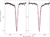 |
Fig. 1. Comparison of observed composite spectra of HD 93028 at opposite phases of maximum separation (in black) with synthetic templates shifted in RVs around the He Iλ5876 spectral line. The individual synthetic spectra for each component are overplotted with dashed blue and green lines, representing the primary and the secondary, respectively. The solid red line corresponds to the combined synthetic spectrum (see Sect. 3.3 for information on the generation of synthetic spectra). |
The major modification to the method involves using a synthetic spectrum as the initial template for the component with narrow and stronger line profiles. This template was selected from the grid of FASTWIND models included in the IACOB Grid-Based Automatic Tool (IACOB-GBAT), based on stellar parameters obtained from a preliminary analysis (see Sect. 3.3) performed on a spectrum closest to quadrature. This synthetic template was then subtracted from the composite spectrum to obtain an initial approximation for the broad-line component, which was used in the first iteration of the disentangling method. Despite these improvements, the resulting reconstructed spectrum for the secondary component is noisy and retains some residuals from the companion.
The disentangling method also provides the RVs of both components for each of the used spectra through the cross-correlation procedure. For this, we used the 3900–7000 Å spectral range, with special care taken around the absorption lines used for spectral analysis, specifically the He I and He II lines present in each system. The RVs of the narrow component were initially measured in He Iλλ4026, 4471, 5015, 5876 and, He IIλλ4542, 4686, 5411. We mainly used He I lines for the broad component.
In the case of HD 101413, HD 151003, and HD 153426, the contribution of each star could not be disentangled. Therefore, we determined the central wavelengths of the spectral lines using the NGAUSS task in IRAF. We used the He I lines at λλ4026, 4471, 5015, 5876, to evaluate the RVs of the narrow components. Since the RVs derived from these lines yielded similar results (maximum differences of 3 km s−1), they were subsequently averaged to represent the RV of the primary component. For the secondary component, the differences were significantly larger, reaching up to 50 km s−1 in a few cases. Consequently, to trace the motion of the secondary, we used the He Iλ5876 line, which, owing to its longer wavelength, provides the best chance to separate the binary components. The RVs were then determined by fitting Gaussian profiles simultaneously to the composite He Iλ5876 line using NGAUSS in IRAF, fixing the widths and intensities to the values obtained from spectra where the components exhibited the largest separation in wavelength.
We compared the RV measurements of the Na I D interstellar lines across all spectra to validate the RV measurements from each spectrograph. In all cases, we found that the RVs of the D1 and D2 lines do not exhibit a systematic difference among spectrographs, and we consider the rms of the mean values as instrumental errors, since these lines are much narrower than the stellar ones.
To estimate the errors in the RVs of the stellar lines, we measured the He Iλ5876 line multiple times in several spectra, varying the limits used for fitting the Gaussian functions. We found that the RVs varied within a range of less than 3 km s−1 for each spectrum obtained with different instrumental configurations. We adopted this value as the typical RV error for the narrow component. Due to the uncertainty in adjusting the line centres for the broader component, we estimated an error of 10 km s−1 (see P18 for further details). The final RVs for the different systems are shown in Appendix A (Tables A.1–A.5 are available online only).
3.2. Orbital solutions
We searched for periodicities in the measured RVs for the narrow-lined component using the interactive NASA Exoplanet Archive Periodogram Service2 employing the Lomb-Scargle method (Scargle 1982). The period ranges and frequency steps were determined by the code. Fig. 2 shows the resulting periodograms for the systems. It is evident from this figure that the period determination is not robust in all cases, as the most probable values do not present significantly higher power compared to others.
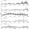 |
Fig. 2. Periodograms obtained from the RVs of the narrow-lined components in the five systems were generated using the NASA Exoplanet Archive Periodogram Service, applying the Lomb-Scargle method. The period ranges and frequency steps are determined by the code, except for HD 153426. Note that, in most cases, the most probable periods, labelled with a red line, are not clearly defined. |
Initially, we ran orbital solutions for the RVs of the narrow component using the GBART code (Bareilles 2017), fixing the period to the value obtained from the Lomb-Scargle analysis. For HD 57236 and HD 101413, their RVs phased with the obtained most probable periods did not represent orbital variability. After inspecting the occurrence of their extreme RVs and testing orbital models with ad hoc periods, we finally obtained very reliable results. Both HD 57236 and HD 101413 turned out to be very eccentric systems, which likely caused the Lomb-Scargle method to fail. In the case of HD 153426, the issue was related to the frequency range selected by the code; adjusting this range yielded the correct value.
Once the periodicities were found, we determined the orbital solution simultaneously for both components using the GBART code and also the FOTEL code (Hadrava 2004), for more eccentric systems, where the convergence of GBART fails. Different datasets were weighted according to their spectral resolution, i.e. the CASLEO RVs were given half the weight of those obtained at LCO and La Silla. The zero-point differences between the different observatory datasets were smaller than 3 km s−1, meaning that no zero-point offset is needed. The derived orbital parameters are provided in Table 2, and the RV curves are shown in Fig. 3.
Orbital solutions for the SB2 systems.
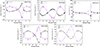 |
Fig. 3. RV curves of the primary (black) and secondary (violet) components of the five binary systems, calculated with the orbital solutions shown in Table 2. RVs from Grunhut et al. (2017, G17) found in the literature were included for the HD 153426 system (green symbols). |
HD 57236 was identified as a double-lined spectroscopic binary (SB2) by Putkuri (2019) and subsequently re-analysed by Mahy et al. (2022). While both studies reached broadly consistent conclusions, discrepancies persist in the determination of K2. In particular, Mahy et al. (2022) derived the secondary velocities through spectral disentangling with most orbital parameters fixed, so that K2 was optimized indirectly rather than measured from individual spectral features.
For HD 93028, the first single-lined (SB1) orbital solution was determined by Levato et al. (1990), who found a circular orbit with a 51.554 d period. The SB2 orbit was later obtained by Putkuri (2019), and more recently by Mahy et al. (2022) using the same methodology as for HD 57236. While their results agree on parameters such as P, e, and K1, they show substantial discrepancies in K2. The large uncertainty in K2 propagates to the derived parameters, leading to poorly constrained masses and a wide uncertainty in q. This underlines how the extraction and measurement of the secondary component become particularly challenging when its spectral contribution is strongly diluted.
HD 101413 was reported as an RV variable by Thackeray & Wesselink (1965) based on three data points obtained at different epochs (1956–1957) with a ΔRV = 98 km s−1. Sana et al. (2011), using 10 high-dispersion spectra from FEROS and UVES found the signature of the secondary component for the first time, though only in the He I lines. They suggested a period of 3 to 6 months and commented that they had never observed such an extreme primary RV as reported by Thackeray & Wesselink (1965) (RVprim = −81 km s−1). The companion spectrum showed neither He II nor Si IV lines, and it was classified as B2-3 V. Based on the He I lines, a mass ratio of 0.17 ± 0.01 was determined, suggesting a mid- to late-B type for the secondary. Putkuri (2019) solved the SB1 system, finding an even longer period, nearly 1000 days in a very eccentric orbit. We closely monitored this system in an effort to capture it during its periastron passage. Unfortunately, the penultimate passage coincided with the COVID-19 pandemic. However, we successfully observed the most recent passage in April 2024. In this work, we present the first SB2 solution for this system. The pair resulted in a wide, highly eccentric orbit (P ∼ 977 d, e ∼ 0.92) which may explain why the secondary has never been adequately detected in the spectra.
HD 151003 was reported as a variable in RV by Conti et al. (1977). Sota et al. (2014) reported it as SB2 with a period of 199 days, according to OWN Survey data.
The RV variability of HD 153426 was first recognized by Crampton (1972), who suspected the SB2 nature of the system. Although the GOSSS data do not reveal double lines, Sota et al. (2011) reported this object as an SB2 system with a period of 22.4 d, based on OWN data, and a preliminary orbital solution was published by Putkuri (2019). Grunhut et al. (2017) analysed spectropolarimetric data to derive line broadening, binary parameters, and magnetic field diagnostics. Two datasets were employed: the first, from July 2011, showed clear evidence of an absorption feature in the red wing of the spectral lines, attributed to a broad-line component in addition to the narrow-line component. However, this broad profile was absent in the second dataset (June 2012). The author’s fits, which maximized the contribution from the broad-line component, matched the first profile well but failed to adequately fit the second profile. Our analysis shows that the RVs of the narrow-line component agree with our orbital solution, while the RVs of the secondary component do not (see the green points in the last plot in Fig. 3). This discrepancy highlights the challenges associated with spectral normalization, particularly for rapidly rotating stars, where line profiles are diluted and blended with the continuum. Careful normalization and high S/N are crucial for obtaining reliable results.
3.3. Spectroscopic analysis
The systems analysed here were spectroscopically classified based on criteria from Sota et al. (2011, 2014) and Maíz Apellániz et al. (2016). To this end, we degraded the best-observed spectrum obtained near quadrature, or the reconstructed spectrum obtained from the disentangling method, to a resolving power R = 2500, in order to compare it with the set of spectra of O-type standards. The main classification criterion for O stars is the helium ionization ratio He IIλ4542/He Iλ4471, but for late-O types, there are other sensitive ratios, such as He IIλ4542/He Iλ4388 and, He IIλ4200/He Iλ4144. We analysed these lines in our systems, and in some cases, we also considered the quantification of classification criteria for spectral types and luminosity classes from Martins (2018), using the measured equivalent widths of classification lines, which were applied to the spectra non-degraded in resolution.
To obtain the fundamental parameters of the stellar components of the systems, i.e. effective temperature (Teff), stellar surface gravity (log g), radius (R), luminosity (L), projected rotational velocity (v sin i), microturbulence (ξT), and others, we employed the IACOB-BROAD tool (Simón-Díaz et al. 2011; Simón-Díaz & Herrero 2014) and the IACOB Grid-Based Automatic Tool (IACOB-GBAT, Simón-Díaz et al. 2011; Sabín-Sanjulián et al. 2014; Holgado et al. 2017, 2018). The IACOB-BROAD tool estimates the contribution of rotational and non-rotational (macroturbulence, vmac) velocities to the line-broadening process, based on a combined Fourier transform and goodness-of-fit methodology. Meanwhile, IACOB-GBAT compares synthetic spectra of He and H, constructed using spectra from the grid of FASTWIND models with solar metallicity (Santolaya-Rey et al. 1997; Puls et al. 2005; Rivero González et al. 2012), with the observed spectrum. As observed spectra, we used the reconstructed ones derived from the spectral disentangling process when available; otherwise, we used the spectra closest to quadrature.
For the quantitative spectroscopic analysis, the observed spectra or reconstructed ones from the disentangling method were scaled by a dilution factor di, ensuring that ∑di = 1. This accounts for the fact that the observed continuum flux in the composite spectrum is the sum of contributions from both stellar components, leading to diluted spectral features that require correction. To address this, the flux ratio between the binary components was taken into consideration. The comparison between observed and synthetic spectra was performed visually as follows: synthetic spectra, initially generated based on the expected stellar parameters for their spectral types, were adjusted by various dilution factors and compared with the observed composite spectrum. We employed IACOB-GBAT to refine the stellar parameters, generate updated synthetic spectra, and recalculate the dilution factors. The spectral lines used in IACOB-GBAT are shown in Table 3.
Spectral lines used for quantitative spectroscopic analysis with IACOB-GBAT tool.
After scaling the individual spectra, we used IACOB-BROAD to determine v sin i and vmac. Although metallic lines are generally preferred for these measurements (as they are less affected by the Stark effect), the He I lines were also considered due to their intensity in O-type stars. This approach was necessary to mitigate the limitations imposed by the S/N (Simón-Díaz & Herrero 2007).
The second step was to determine the effective temperatures and gravities. The synthetic spectra of each component were convolved with the corresponding v sin i and vmac, shifted in RV, and scaled by the appropriate dilution factor. The helium surface abundance and the exponent of the wind-velocity law were fixed to typical values for Galactic mid-O-type dwarfs (namely, helium abundance YHe = 0.10 and the exponent of the wind velocity-law β = 0.8). Since broadened-line components appear more diluted in the spectra, and some lines are even indistinguishable, only a subset of the available lines was used for these components. The selected lines are highlighted in coloured cells in Table 3.
The log g values should be taken with caution, as they are derived from the wings of the Balmer lines, which are affected by the blending of both stellar components. In these particular binaries, this effect is further complicated by the broadening of the spectral lines from the secondary component. The gravity corrected from rotational velocity, log gc (see e.g. Herrero et al. 1992; Repolust et al. 2004), is not considered in this analysis because there is a range of log g values observed in the secondary components, and because the correction in the primary component is negligible.
Once Teff and log g were determined, we used them, along with the absolute magnitude of each component (MV), to obtain the radius (R), luminosity (L), and spectroscopic mass (Msp). We calculated the absolute magnitudes of the O-type stars using “observational” MV values derived from (1) extinction-corrected visual magnitudes from Maíz Apellániz & Barbá (2018), (2) distances provided by the ALS III catalogue (Pantaleoni González et al. 2025), and (3) the flux ratios obtained in this work. The results for the five systems are shown in Table 4. A brief description of each system is given in the following.
3.3.1. HD 57236
HD 57236 was classified as O8 V((f)) by Walborn (1982), and O8.5 V, based on the new criteria (Sota et al. 2014). Maíz Apellániz et al. (2016) considered it a standard of this spectral type. In this work, we visually inspected some composite spectra obtained near quadratures to perform a spectroscopic classification.
For the primary component, we used the reconstructed spectrum obtained from the disentangling method to provide a more accurate estimation of the spectral type. The ratios He IIλ4542/He Iλ4388 and He IIλ4200/He Iλ4144 are both greater than unity, indicating an O8–8.5 subtype. Additionally, considering the quantification of classification criteria (see Sect. 3.3), we found agreement with the O8 type. By analysing the strong He IIλ4686 absorption line, both in the reconstructed spectrum and in the synthetic one for this component (see the blue profile in Fig. A.1), we determined an equivalent width (EW) between 0.5 Å and 0.8 Å, consistent with luminosity classes V, IV, and III. On the other hand, we obtained a Vz classification using the quantitative criterion proposed by Arias et al. (2016), which states that the ratio of the equivalent width of He IIλ4686 line to the maximum between the equivalent widths of the He Iλ4471 and He IIλ4542 must be greater or equal to 1.1.
Regarding the secondary component, the spectral classification is more challenging due to the lower S/N obtained with the disentangling method. Additionally, it is affected by some spurious artefacts (mainly in the wings of the Balmer lines), and this issue is amplified due to the very broad lines. Nevertheless, the presence of He Iλ4471 and He Iλ4388 can be clearly noted, while the He IIλ4542 is marginally detected. Considering the non-detection of Si IVλ4552, we constrain the spectral type in the range O9.5 – O9.7. Taking into account the O9–O9.7 luminosity criteria from Sota et al. (2011), we found that the secondary component could belong to the luminosity classes V or III. We evaluated the EW of He IIλ4686, He Iλ4713 and He I+IIλ4026 synthetic lines of the secondary component (see red line in Fig. A.1) and concluded that luminosity class V is more appropriate.
Therefore, the binary system HD 57236 comprises an O8 IV primary and an O9.5–09.7 V(n) secondary. The ‘(n)’ qualifier for the secondary is added to account for the broadening of its spectral features, with v sin i ≥ 200 km s−1.
To determine the stellar parameters, we analysed the O IIIλ5592 and He Iλλ5876, 5015 and 4713 lines in the reconstructed spectrum of the primary component and determined that v sin i is not greater than 30 km s−1 and vmac is about 50 km s−1. The best fit was obtained for O IIIλ5592, yielding v sin i = 27.3 ±1.3 km s−1 and vmac = 47.6 ±1.3 km s−1 which were the adopted values for these parameters. Simón-Díaz & Herrero (2014) showed that velocities below 40 km s−1 (low-velocity regime) must be considered as an upper limit to the actual velocities because these values may be produced by microturbulence. For the secondary component, we employed the composite spectra near quadratures for analysing the He Iλλ5876, 4388, and 4922; and Si IVλ4089. In this case, we subtracted the reconstructed spectrum of the primary and analysed the resulting spectrum. We obtained v sin i = 225 ±10 km s−1 and vmac = 57 ±10 km s−1 (consistent with the (n) qualifier in the spectral type).
Table 4 presents the results derived for both stellar components of the system, and Fig. A.1 shows a comparison between the synthetic (green) and observed (grey) composite spectra at orbital phase 0.99. The synthetic spectrum was constructed using the best-fitting FASTWIND models obtained for each component (blue for the primary, with Teff = 36 000 K, log g = 3.7 dex, and log Q = −12.7; red for the secondary, with Teff = 34 000 K, log g = 4.0 dex, and log Q = −12.7)3. Before combining them, each model was shifted in RV and scaled according to the flux ratio. We found the flux ratio LB/LA = 0.30/0.70 ∼ 0.42, meaning that 70 (30) per cent of the total light corresponds to the primary (secondary) component. The figure illustrates the quality of the best-fitting solution and the good determination of RVs and dilution factors. The relative contribution of each component to the global spectrum is also visible. The ratio of spectroscopic masses (q < 0.89) agrees with the q parameter obtained from the dynamical solution.
3.3.2. HD 93028
HD 93028 (CPD −59 2521) was initially classified as O9 V by Walborn (1972), but Sota et al. (2011) later reclassified it as O9 IV and designated it as the MK standard star for this spectral subtype. Using the reconstructed spectrum of the primary component obtained through the disentangling method, we analysed the spectral classification and found concordance with the reclassification by Sota et al. (2011). This result suggests that the contribution of the secondary component to the composite spectrum is marginal. The disentangled spectrum of the primary is shown in Fig. 4. This figure serves to illustrate both the spectral lines relevant to the classification and the visual inspection, and the quality of the disentangling method.
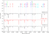 |
Fig. 4. Disentangled spectrum of the primary component of HD 93028 (in red), compared with GOSSS O-type standard spectra for the same spectral range (in black). Key spectral features are labelled. This figure exemplifies the classification procedure applied to all stars analysed in this work. |
Regarding the secondary component, the low S/N of the spectrum prevents a detailed analysis. Therefore, we opted to visually inspect some spectra obtained near quadrature phases. In these spectra, He Iλλ4026, 4388, 4471, 4922, 5015, 5876, 6678 are present. No features from He II, or metallic lines are detected. Based on this, we classify the secondary as a B-type star, with the qualifier ‘(n)’ to indicate broad lines typical of fast rotation.
To estimate the line-broadening parameters, we analysed the Si IIIλ4552, O IIIλ5592 and He Iλλ5015, 4713 lines for the primary component. For the secondary component, metallic lines were not distinguishable in the reconstructed spectrum, so we fitted the He I lines (λλ5015, 5876, and 4922) instead. The dilution factor in this system was found to be 85% (primary) and 15% (secondary) in the global spectrum. For the primary component, we obtained v sin i = 29 ± 2 km s−1 and vmac = 48 ± 2 km s−1. For the secondary component, we derived a relatively high projected rotational velocity of v sin i = 153 ± 8 km s−1 and vmac = 45 ± 8 km s−1. We consider velocities ≤40 km s−1 to be an upper limit.
To calculate the fundamental parameters, we estimate the MV of the primary component as described in Sect. 3.3. Based on the flux ratio derived from the orbital solution, we estimated an MV of −2.47 mag for the secondary component, which is compatible with a B1.5 – B2 spectral type.
Finally, we compare the parameters of the primary component with those of the ALS 12502 Aa (Ansín et al. 2023), a star with the same spectral type that belongs to an eclipsing binary system. For this object, Ansín et al. (2023) derived a spectroscopic mass of Msp = 21.64 ± 7.8 M⊙, luminosity of log L = 4.79±0.04, and radius of R = 8.64 ± 1.19 R⊙. Our determination for the O9 IV component in HD 93028 is close to these empirical values, except the comparison between our spectroscopic mass with the dynamic one determined by them (see Table 4).
Parameters determined from the spectroscopic analysis for the SB2 systems. The ξT denotes the microturbulence velocity.
3.3.3. HD 101413
HD 101413 (CPD –62 2205) is the visual companion of HD 101436, with a separation of 27.8 arcseconds (Mason et al. 1998). Walborn (1973) classified HD 101413 as O8 V. In this study, we used a spectrum obtained at RV maximum and found agreement with this classification. For the secondary component, we visually inspected some spectra obtained near quadratures. These spectra revealed absorption lines of He Iλλ4026, 4471, 4922 and 5876, but no He II features or metallic lines were detected. Based on these observations, we classified the secondary component as early-B.
Previous studies have reported the v sin i of HD 101413 based on IUE spectra. Penny (1996) derived 102 km s−1, Howarth et al. (1997) found 99 km s−1, and Stickland & Lloyd (2001) reported 98 km s−1. Using optical spectra, Conti & Ebbets (1977) determined v sin i ∼ 140 km s−1, Daflon et al. (2007) reported 136 ± 17 km s−1, and Williams et al. (2011) found 149 ± 17 km s−1. These optical measurements are systematically higher than those obtained from the IUE data. Williams et al. (2011) suggested that the discrepancy in v sin i values might indicate that HD 101413 is an unresolved double-lined system.
We analysed the line-broadening parameters for the primary component using the C IVλλ5801, 5811, as these lines are probably not affected by the companion. The mean values obtained were 83±5 km s−1 and 60±5 km s−1 for the v sin i and vmac, respectively. The spectroscopic analysis for the primary component was carried out on the observed spectrum near quadrature, with the contribution of the companion removed. Next, we used the IACOB-GBAT tool to generate a synthetic spectrum for the broad component, ensuring that the sum of both spectra matched the composite observed spectrum. In the first step, we used the stellar parameters expected for their spectral type. From this, we determined that approximately 75 percent of the total light corresponds to the primary component, and the flux ratio (FB/FA) is about 0.33. The results are listed in Table 4. Fig. A.2 shows the fit for some spectral lines. The parameters obtained for the broad component should be considered as approximate.
Taking into account the flux ratio of the system from the dynamical solution and the MV for the primary component, we derived MV = −3.13 for the secondary component. This value corresponds to a B1 star according to Bowen et al. (2008). This result is consistent with the mass ratio q ∼ 0.63, and the non-detection of He II lines may be attributed to dilution from the fast rotation of the secondary component.
3.3.4. HD 151003
HD 151003 (CPD –41 7600) was classified as O8.5 III by Sota et al. (2014). In this study, we performed a visual inspection to determine the spectral classification of both components.
For the narrow component, we additionally measured the equivalent widths of the diagnostic lines in the robust disentangled spectrum, yielding a spectral type of O8 III. The reconstructed spectrum of the secondary component, however, is significantly affected by spurious artefacts, preventing a reliable spectral classification based on quantitative line-strength ratios. Nevertheless, several absorption features can still be identified in this spectrum, including He Iλλ4026, 4388, 4471, 4713, 4922, 5015, 5876, 6678, and 7065, He IIλλ4200, 4542, 4686 and 5411, as well as some metallic lines (e.g. Si Iλ4089). Although the presence of these lines indicates that both components share broadly similar spectral characteristics, the limited quality of the secondary spectrum only allows us to qualitatively suggest a late-O spectral subtype for the broad component. Its luminosity class could not be constrained.
Sana et al. (2014), using the PIONIER instrument at the Very Large Telescope, detected a companion at a separation of ρ = 1.85±0.14 mas and with a magnitude difference of ΔH = 1.12±0.02 mag (A,B pair). A faint companion (A,C) was also detected with NACO-FOV. Given the distance of 1562 pc (Bailer-Jones et al. 2021), the most likely value for the separation of 1.85 mas corresponds to a physical separation of approximately 620 R⊙. The observed epoch of the measurements (2012.4441) corresponds to an orbital phase of ϕ = 0.43, and the projected separation between components is estimated to be about 600 R⊙, according to our orbital solution. This indicates that the interferometric component coincides with the spectroscopic discovery presented here. On the other hand, if we analysed the MV of the secondary component based on the calculated MV of the primary component, we found approximately −4.78 mag, corresponding to a star with spectral type O9 or later, and a luminosity class III.
Taking into account the mass ratio q, the system appears to consist of an O8 III primary and a late-O III secondary. Fig. A.3 shows a composite spectrum near quadrature, compared to combined synthetic models. The projected rotational ratio is noteworthy. The parameters of the secondary component were derived by fitting the observed spectrum with combined synthetic models, using the previously determined parameters for the primary component.
3.3.5. HD 153426
HD 153426 (CPD –38 6624) is a field star, according to Gies (1987), with an O8.5 III spectral-type (Sota et al. 2014; Martins 2018). Our analysis of the primary component’s spectrum confirms its O8.5 III classification. This aligns with the observation that the contribution of the secondary component to the composite spectrum is marginal, as is shown in Fig. A.4.
Regarding the secondary component, we visually inspected spectra obtained near quadratures, identifying absorption lines from He Iλλ4026, 4388, 4471, 4713, 4922, 5015, 5876, 6678, and 7065, together with marginal detections of He IIλλ4200, 4542, 4686 and 5411, lines. We conclude that the spectrum of the secondary component is consistent with an early B-type classification. Considering the flux ratio determined from the dynamical solution, the absolute magnitude of the secondary is estimated to be −4.1 mag, placing it within the late-O to early-B spectral range (Bowen et al. 2008).
For the broadening parameters, we analysed several He I and metallic lines. However, the presence of residuals of the secondary component in the primary component reconstructed spectrum led to an overestimation of the vmac. The less affected lines, Si IVλλ4116 and 4089, were used to estimate the broadening parameters. From these, we determined the v sin i of the primary component to be 92±5 km s−1 and vmac to be 65 ±5 km s−1.
For the secondary, we employed the reconstructed spectrum obtained from the disentangling method and measured the broadening parameters in He Iλλ5015 and 5876 lines. The values obtained were v sin i = 217±12 km s−1 and vmac = 100 ±12 km s−1.
We find that approximately 65 percent of the total light in the system corresponds to the primary component. We then scaled adequately the synthetic templates of HD 153426 for the spectroscopic analyses. In Fig. A.4 we show the contribution of both components at one composite spectrum.
3.4. Photometric analysis
The five systems examined in this study were observed by the Transiting Exoplanet Survey Satellite (TESS). Given their eccentric orbital configurations, particular attention was given to potential photometric variations near periastron passage, where tidal interactions and reflection effects would be most pronounced. We performed aperture photometry on 21 × 21 pixel cutouts, removing systematic noise through regression analysis and computing periodograms. All photometric processing was conducted using the Lightkurve package (Lightkurve Collaboration, 2018). It should be noted that three systems (HD 57236, HD 93028, and HD 101413) lacked observational coverage during periastron passage. No significant variability correlated with the orbital phase was detected in any of these systems. The light curve of HD 57236, observed across four sectors, exhibited stochastic variations at the 0.1% level without detectable periodicity. For HD 93028, observations spanning six sectors were significantly affected by contamination from nearby sources, including an eclipsing binary within the photometric aperture. A similar situation was observed in the light curve of HD 101413, which, when analysed using data from five sectors in a crowded field, displayed variability patterns that could not be conclusively attributed to the target star. The analysis was thus focused on HD 151003 and HD 153426, the only systems with observational coverage near periastron. While HD 151003 (three sectors) is relatively isolated, its photometry was affected by gaps in the data resulting from images being removed during the calibration phase.
No significant variability (< 1% amplitude) was detected during periastron passage in Sector 12 observations. In contrast, the short-period system HD 153426 (observed in three sectors) provided comprehensive orbital phase coverage, yet exhibited only faint (0.2% amplitude) variations that showed no correlation with the orbital phase. The absence of detected photometric variations may be indicative of intrinsically weak tidal or reflection effects, or of unfavourable system geometries.
3.5. Evolutionary status
To study the evolutionary status of the systems, we computed a set of evolutionary tracks corresponding to solar composition models. The masses were selected to cover the relevant region of the HRD and have been set logarithmically evenly spaced with a step of 20%. We employed the code presented in Benvenuto & De Vito (2003), to which it has been added the treatment of shellular rotation, as briefly described in the Appendix of Putkuri et al. (2022). The results are presented in Fig. 5, where models without rotation are denoted with black lines whereas red lines depict rotating models with a tangential equatorial velocity of 300 km s−1 at the ZAMS. The isochrones of 0(1)10 Myr have also been indicated (see the corresponding caption for the lines code).
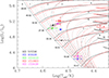 |
Fig. 5. Theoretical HR diagram for massive stars together with the data corresponding to the binaries studied in this paper. All models have solar composition. The mass values are logarithmically evenly spaced with a step of 20% and are given in solar units at the left of the start of each track near the ZAMS. Models without rotation are denoted with black lines, whereas red lines depict rotating models with a tangential equatorial velocity of 300 km s−1 at the ZAMS. Solid lines show the evolutionary tracks, whereas isochrones are denoted by solid (0 [i.e. the ZAMS], 5, and 10 Myr), dotted (1 and 6 Myr), short dashed (2 and 7 Myr), long dashed (3 and 8 Myr), and dash-dotted lines (4 and 9 Myr), respectively. The secondaries of the systems HD 101413 and HD 153426 overlap. |
In Table 5 we present the evolutionary masses and ages of the components of the systems studied in this paper. The masses and ages correspond to the comparison of photometric data against the set of rotating and non-rotating models. Mi correspond to the present-day mass of a star of Agei and initial mass  on the ZAMS. For its part, i = r (i = nr) correspond to models with (without) rotation. All objects are very young and massive. In general, taking into account the size of the uncertainties, we find that the ages of the primary and secondary components are similar. Indeed, while employing models with rotation we get higher masses and lower ages than those we would find if based on non-rotating ones. The error bars are larger than the differences.
Some characteristics of the components of the binary systems studied in this paper.
Given that the systems are young, as we have shown, we explored the origin of asynchronous rotation just as done in P22, and considered mass transfer scenarios. We observed that the stars studied here, are well separated during most of the orbital period, except during periastron, when components are closer due to high eccentricity. Then, the parameter that describes the Roche Lobe filling percentage (RA + RB)/a changes with the orbital phases.
Hamers & Dosopoulou (2019) developed an analytic model for the secular orbital evolution of binaries undergoing conservative mass transfer. They categorized mass transfer based on two orbital parameters (q and a) and the radius of the donor star (R). The x parameter is defined as x = RL/R4, where RL is the Roche lobe radius in a circular orbit (Eggleton 1983). For simplicity, we assumed an inclination angle of 90° (a sin i = a) for the analysis. Considering the dynamical and spectroscopic masses, the inclination angle is greater than 50° in all cases, and the results are not qualitatively affected. If the inclination were smaller, the semi-axes would be larger (up to 30%), but in all cases the status of each system regarding mass transfer is firmly established.
Through the x parameter, it can be seen if the donor star fills its Roche lobe during the entire orbit (full Roche lobe overflow (RLOF)), or fills it during part of the orbit (partial RLOF), or does not fill it (No RLOF). In Fig. 6 we plotted the x parameter for the five systems, and found that all points fall in the region of No RLOF. Thus, none of these systems undergo RLOF in any part of their orbits.
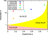 |
Fig. 6. Regimes of mass transfer from Hamers & Dosopoulou (2019) in the (e, x) plane. The coloured regions correspond different regimes of mass transfer in eccentric orbits. None of the systems studied in this paper undergo mass transfer in any portion of their orbits. |
4. Discussion and final remarks
In this work, we determined the SB2 orbits of the massive systems HD 57236, HD 93028, HD 101413, HD 151003, and HD 153426, using the available multi-epoch, high-resolution optical spectroscopy gathered by the OWN Survey. We found that these systems have wide and eccentric orbits, with orbital periods longer than 190 d, except for HD 153426, which has a much shorter period of ∼22 d. The orbital eccentricities range from 0.1457 to 0.924, with HD 101413 exhibiting one of the most eccentric orbits among known massive binary systems. Highly eccentric binaries are challenging to detect because they spend only a small fraction of their time near the periastron, where they exhibit significant RV variations (see Fig. 3). Additionally, the sample analysed here consists of systems with a component showing high rotational broadening (v sin i ⪆ 200 km s−1), which further reduces our ability to detect them. A high cadence of observations and high resolution are necessary for accurate detection of the secondary spectrum. We analysed the eccentricities as a function of the orbital period for the five systems, and no clear trend between these parameters was found. However, we highlight the proximity of HD 101413 to the instability region (see Fig. 3 in Moe & Di Stefano 2017).
In addition to the orbital analysis, we performed a quantitative spectral and evolutionary analysis (see Tables 4 and 5). To assess the evolutionary status of the stars, we applied models that account for rotation. We found that the components of each system are consistent with a common age between ∼1 to 4 Ma. This means that a population of young, massive stars can have high rotational velocities without having undergone significant alteration through binary evolution.
Additionally, since no overflow has occurred yet (see Sect. 3.5), the faster rotation is a consequence of their formation, indicating that binary interaction is not the only pathway to high rotational velocities in massive stars. The stars in these systems likely acquired their angular momentum during the star formation process.
In general, we must exercise caution and intensify our study of the non-negligible percentage of massive O-type stars rotating at high velocities (see for example Britavskiy et al. 2023). The theoretical models will differ depending on whether the stars acquired their angular momentum during the star formation process or through a past interaction episode in a binary system.
Our results, which indicate that the angular momentum of the rapid rotators was primarily acquired during star formation, are consistent with the conclusions of Britavskiy et al. (2024), who investigated short-period, extreme mass-ratio binaries and likewise favoured a primordial origin for rapid rotation, while also considering alternative scenarios such as spin-up through mass transfer or mergers in hierarchical triple systems. Interestingly, in our sample the rapid rotator is always the less massive component, whereas in the systems studied by Britavskiy et al. (2024) it is the more massive star. This contrast suggests that different mechanisms may dominate in different regions of parameter space, or that the role of stellar mass in the acquisition and preservation of angular momentum remains incompletely understood, reinforcing the idea that rotation alone is not a sufficient tracer of past binary interactions. Currently, the discussion is ongoing, but we believe it is clear that the binary interaction is not the only channel for rapid rotation in massive stars.
Data availability
This paper is based on spectroscopic data belonging to the OWN Survey and IACOB Project, available upon reasonable request from Dr Roberto Gamen and Dr Sergio Simón-Díaz.
Tables A.1–A.5 in the Appendix are available at the CDS via https://cdsarc.cds.unistra.fr/viz-bin/cat/J/A+A/706/A311.
Figures A.1–A.4 in the Appendix are publicly available on Zenodo DOI:10.5281/zenodo.18242194.
Acknowledgments
We thank the anonymous referee for a thorough reading of the manuscript, which helped to improve its quality. CP and RG acknowledge support from grant PICT 2019-0344. CP and RG are Visiting Astronomers of the CASLEO, and Las Campanas Observatory, and RG, of La Silla/ESO. OGB is member of the Carrera del Investigador Científico of the Comisión de Investigaciones Científicas de la Provincia de Buenos Aires (CICPBA), Argentina. We thank the directors and staff of CASLEO, LCO, and La Silla/ESO for support and hospitality during our observing runs. This research has made use of the SIMBAD database, operated at CDS, Strasbourg, France. This research has made use of the NASA Exoplanet Archive, which is operated by the California Institute of Technology, under contract with the National Aeronautics and Space Administration under the Exoplanet Exploration Program. This work has made use of data from the European Space Agency (ESA) mission Gaia (https://www.cosmos.esa.int/gaia), processed by the Gaia Data Processing and Analysis Consortium (DPAC, https://www.cosmos.esa.int/web/gaia/dpac/consortium). Funding for the DPAC has been provided by national institutions, in particular, the institutions participating in the Gaia Multilateral Agreement. J. I. A acknowledges the financial support from the Dirección de Investigación y Desarrollo de la Universidad de La Serena (ULS), through the project PR2324063.
References
- Ansín, T., Gamen, R., Morrell, N. I., et al. 2023, MNRAS, 525, 4566 [CrossRef] [Google Scholar]
- Arias, J. I., Walborn, N. R., Simón Díaz, S., et al. 2016, AJ, 152, 31 [NASA ADS] [CrossRef] [Google Scholar]
- Bailer-Jones, C. A. L., Rybizki, J., Fouesneau, M., Demleitner, M., & Andrae, R. 2021, AJ, 161, 147 [Google Scholar]
- Barbá, R. H., Gamen, R., Arias, J. I., & Morrell, N. I. 2017, IAU Symp., 329, 89 [Google Scholar]
- Bareilles, F. 2017, GBART: Determination of the orbital elements of spectroscopic binaries [Google Scholar]
- Benvenuto, O. G., & De Vito, M. A. 2003, MNRAS, 342, 50 [NASA ADS] [CrossRef] [Google Scholar]
- Bersten, M. C., Benvenuto, O. G., Orellana, M., & Nomoto, K. 2016, ApJ, 817, L8 [NASA ADS] [CrossRef] [Google Scholar]
- Bowen, D. V., Jenkins, E. B., Tripp, T. M., et al. 2008, ApJS, 176, 59 [NASA ADS] [CrossRef] [Google Scholar]
- Britavskiy, N., Simón-Díaz, S., Holgado, G., et al. 2023, A&A, 672, A22 [NASA ADS] [CrossRef] [EDP Sciences] [Google Scholar]
- Britavskiy, N., Renzo, M., Nazé, Y., Rauw, G., & Vynatheya, P. 2024, A&A, 684, A35 [NASA ADS] [CrossRef] [EDP Sciences] [Google Scholar]
- Chrimes, A. A., Stanway, E. R., & Eldridge, J. J. 2020, MNRAS, 491, 3479 [NASA ADS] [CrossRef] [Google Scholar]
- Clark, J. S., Ritchie, B. W., Najarro, F., Langer, N., & Negueruela, I. 2014, A&A, 565, A90 [NASA ADS] [CrossRef] [EDP Sciences] [Google Scholar]
- Conti, P. S., & Ebbets, D. 1977, ApJ, 213, 438 [CrossRef] [Google Scholar]
- Conti, P. S., Leep, E. M., & Lorre, J. J. 1977, ApJ, 214, 759 [Google Scholar]
- Crampton, D. 1972, MNRAS, 158, 85 [NASA ADS] [Google Scholar]
- Daflon, S., Cunha, K., de Araújo, F. X., Wolff, S., & Przybilla, N. 2007, AJ, 134, 1570 [NASA ADS] [CrossRef] [Google Scholar]
- Díaz-Rodríguez, M., Murphy, J. W., Williams, B. F., Dalcanton, J. J., & Dolphin, A. E. 2021, MNRAS, 506, 781 [CrossRef] [Google Scholar]
- Dorn-Wallenstein, T. Z., & Levesque, E. M. 2020, ApJ, 896, 164 [Google Scholar]
- Eggleton, P. P. 1983, ApJ, 268, 368 [Google Scholar]
- Gies, D. R. 1987, ApJS, 64, 545 [NASA ADS] [CrossRef] [Google Scholar]
- González, J. F., & Levato, H. 2006, A&A, 448, 283 [NASA ADS] [CrossRef] [EDP Sciences] [Google Scholar]
- Grunhut, J. H., Wade, G. A., Neiner, C., et al. 2017, MNRAS, 465, 2432 [NASA ADS] [CrossRef] [Google Scholar]
- Hadrava, P. 2004, Publications of the Astronomical Institute of the Czechoslovak. Academy of Sciences, 92, 1 [Google Scholar]
- Hamers, A. S., & Dosopoulou, F. 2019, ApJ, 872, 119 [NASA ADS] [CrossRef] [Google Scholar]
- Herrero, A., Kudritzki, R. P., Vilchez, J. M., et al. 1992, A&A, 261, 209 [NASA ADS] [Google Scholar]
- Holgado, G., Simón-Díaz, S., & Barbá, R. 2017, IAU Symp., 329, 407 [Google Scholar]
- Holgado, G., Simón-Díaz, S., Barbá, R. H., et al. 2018, A&A, 613, A65 [NASA ADS] [CrossRef] [EDP Sciences] [Google Scholar]
- Howarth, I. D., Siebert, K. W., Hussain, G. A. J., & Prinja, R. K. 1997, MNRAS, 284, 265 [NASA ADS] [CrossRef] [Google Scholar]
- Kasen, D., & Bildsten, L. 2010, ApJ, 717, 245 [NASA ADS] [CrossRef] [Google Scholar]
- Levato, H., Malaroda, S., García, B., Morrell, N., & Solivella, G. 1990, ApJS, 72, 323 [Google Scholar]
- Mahy, L., Sana, H., Shenar, T., et al. 2022, A&A, 664, A159 [NASA ADS] [CrossRef] [EDP Sciences] [Google Scholar]
- Maíz Apellániz, J., & Barbá, R. H. 2018, A&A, 613, A9 [Google Scholar]
- Maíz Apellániz, J., Sota, A., Arias, J. I., et al. 2016, ApJS, 224, 4 [CrossRef] [Google Scholar]
- Martins, F. 2018, A&A, 616, A135 [NASA ADS] [CrossRef] [EDP Sciences] [Google Scholar]
- Mason, B. D., Gies, D. R., Hartkopf, W. I., et al. 1998, AJ, 115, 821 [NASA ADS] [CrossRef] [Google Scholar]
- Mazzali, P. A., McFadyen, A. I., Woosley, S. E., Pian, E., & Tanaka, M. 2014, MNRAS, 443, 67 [Google Scholar]
- Metzger, B. D., Thompson, T. A., & Quataert, E. 2007, ApJ, 659, 561 [Google Scholar]
- Meynet, G., & Maeder, A. 2000, A&A, 361, 101 [NASA ADS] [Google Scholar]
- Moe, M., & Di Stefano, R. 2017, ApJS, 230, 15 [Google Scholar]
- Orellana, M., Bersten, M. C., & Moriya, T. J. 2018, A&A, 619, A145 [NASA ADS] [CrossRef] [EDP Sciences] [Google Scholar]
- Pantaleoni González, M., Maíz Apellániz, J., Barbá, R. H., et al. 2025, MNRAS, 543, 63 [Google Scholar]
- Penny, L. R. 1996, ApJ, 463, 737 [Google Scholar]
- Puls, J., Urbaneja, M. A., Venero, R., et al. 2005, A&A, 435, 669 [NASA ADS] [CrossRef] [EDP Sciences] [Google Scholar]
- Putkuri, C. E. 2019, Ph.D. Thesis (Argentina: National University of La Plata) [Google Scholar]
- Putkuri, C., Gamen, R., Morrell, N. I., et al. 2018, A&A, 618, A174 [NASA ADS] [CrossRef] [EDP Sciences] [Google Scholar]
- Putkuri, C., Gamen, R., Morrell, N. I., et al. 2021, A&A, 650, A96 [NASA ADS] [CrossRef] [EDP Sciences] [Google Scholar]
- Putkuri, C., Gamen, R., Benvenuto, O. G., et al. 2022, MNRAS, 517, 3101 [Google Scholar]
- Rauw, G. 2024, Bulletin de la Societe Royale des Sciences de Liege, 93, 58 [Google Scholar]
- Repolust, T., Puls, J., & Herrero, A. 2004, A&A, 415, 349 [NASA ADS] [CrossRef] [EDP Sciences] [Google Scholar]
- Rivero González, J. G., Puls, J., Massey, P., & Najarro, F. 2012, A&A, 543, A95 [NASA ADS] [CrossRef] [EDP Sciences] [Google Scholar]
- Sabín-Sanjulián, C., Simón-Díaz, S., Herrero, A., et al. 2014, A&A, 564, A39 [NASA ADS] [CrossRef] [EDP Sciences] [Google Scholar]
- Sana, H., James, G., & Gosset, E. 2011, MNRAS, 416, 817 [Google Scholar]
- Sana, H., Le Bouquin, J.-B., Lacour, S., et al. 2014, ApJS, 215, 15 [Google Scholar]
- Santolaya-Rey, A. E., Puls, J., & Herrero, A. 1997, A&A, 323, 488 [NASA ADS] [Google Scholar]
- Scargle, J. D. 1982, ApJ, 263, 835 [Google Scholar]
- Simón-Díaz, S., & Herrero, A. 2007, A&A, 468, 1063 [NASA ADS] [CrossRef] [EDP Sciences] [Google Scholar]
- Simón-Díaz, S., & Herrero, A. 2014, A&A, 562, A135 [NASA ADS] [CrossRef] [EDP Sciences] [Google Scholar]
- Simón-Díaz, S., Castro, N., Herrero, A., et al. 2011, J. Phys. Conf. Ser., 328, 012021 [Google Scholar]
- Sota, A., Maíz Apellániz, J., Walborn, N. R., et al. 2011, ApJS, 193, 24 [Google Scholar]
- Sota, A., Maíz Apellániz, J., Morrell, N. I., et al. 2014, ApJS, 211, 10 [Google Scholar]
- Stickland, D. J., & Lloyd, C. 2001, The Observatory, 121, 1 [NASA ADS] [Google Scholar]
- Thackeray, A. D., & Wesselink, A. J. 1965, MNRAS, 131, 121 [Google Scholar]
- Thompson, T. A., Chang, P., & Quataert, E. 2004, ApJ, 611, 380 [NASA ADS] [CrossRef] [Google Scholar]
- Walborn, N. R. 1972, AJ, 77, 312 [NASA ADS] [CrossRef] [Google Scholar]
- Walborn, N. R. 1973, AJ, 78, 1067 [NASA ADS] [CrossRef] [Google Scholar]
- Walborn, N. R. 1982, AJ, 87, 1300 [NASA ADS] [CrossRef] [Google Scholar]
- Williams, S. J., Gies, D. R., Helsel, J. W., Matson, R. A., & Caballero-Nieves, S. 2011, AJ, 142, 5 [Google Scholar]
- Woosley, S. E. 2010, ApJ, 719, L204 [NASA ADS] [CrossRef] [Google Scholar]
IRAF is distributed by the National Optical Astronomy Observatories, which are operated by the Association of Universities for Research in Astronomy, Inc., under a cooperative agreement with the National Science Foundation.
See Simón-Díaz et al. (2011) for information about the ranges of values considered for the free parameters in the FASTWIND grid.
RL = a (0.49 q2/3)/(0.6 q2/3 + ln(1 + q1/3)).
All Tables
Details of the collected spectroscopic data for the five systems (R stands for the spectral resolving power, and n for the number of spectra gathered with each instrument.
Spectral lines used for quantitative spectroscopic analysis with IACOB-GBAT tool.
Parameters determined from the spectroscopic analysis for the SB2 systems. The ξT denotes the microturbulence velocity.
Some characteristics of the components of the binary systems studied in this paper.
All Figures
|
Fig. 1. Comparison of observed composite spectra of HD 93028 at opposite phases of maximum separation (in black) with synthetic templates shifted in RVs around the He Iλ5876 spectral line. The individual synthetic spectra for each component are overplotted with dashed blue and green lines, representing the primary and the secondary, respectively. The solid red line corresponds to the combined synthetic spectrum (see Sect. 3.3 for information on the generation of synthetic spectra). |
| In the text | |
|
Fig. 2. Periodograms obtained from the RVs of the narrow-lined components in the five systems were generated using the NASA Exoplanet Archive Periodogram Service, applying the Lomb-Scargle method. The period ranges and frequency steps are determined by the code, except for HD 153426. Note that, in most cases, the most probable periods, labelled with a red line, are not clearly defined. |
| In the text | |
|
Fig. 3. RV curves of the primary (black) and secondary (violet) components of the five binary systems, calculated with the orbital solutions shown in Table 2. RVs from Grunhut et al. (2017, G17) found in the literature were included for the HD 153426 system (green symbols). |
| In the text | |
|
Fig. 4. Disentangled spectrum of the primary component of HD 93028 (in red), compared with GOSSS O-type standard spectra for the same spectral range (in black). Key spectral features are labelled. This figure exemplifies the classification procedure applied to all stars analysed in this work. |
| In the text | |
|
Fig. 5. Theoretical HR diagram for massive stars together with the data corresponding to the binaries studied in this paper. All models have solar composition. The mass values are logarithmically evenly spaced with a step of 20% and are given in solar units at the left of the start of each track near the ZAMS. Models without rotation are denoted with black lines, whereas red lines depict rotating models with a tangential equatorial velocity of 300 km s−1 at the ZAMS. Solid lines show the evolutionary tracks, whereas isochrones are denoted by solid (0 [i.e. the ZAMS], 5, and 10 Myr), dotted (1 and 6 Myr), short dashed (2 and 7 Myr), long dashed (3 and 8 Myr), and dash-dotted lines (4 and 9 Myr), respectively. The secondaries of the systems HD 101413 and HD 153426 overlap. |
| In the text | |
|
Fig. 6. Regimes of mass transfer from Hamers & Dosopoulou (2019) in the (e, x) plane. The coloured regions correspond different regimes of mass transfer in eccentric orbits. None of the systems studied in this paper undergo mass transfer in any portion of their orbits. |
| In the text | |
Current usage metrics show cumulative count of Article Views (full-text article views including HTML views, PDF and ePub downloads, according to the available data) and Abstracts Views on Vision4Press platform.
Data correspond to usage on the plateform after 2015. The current usage metrics is available 48-96 hours after online publication and is updated daily on week days.
Initial download of the metrics may take a while.