| Issue |
A&A
Volume 706, February 2026
|
|
|---|---|---|
| Article Number | A130 | |
| Number of page(s) | 14 | |
| Section | Galactic structure, stellar clusters and populations | |
| DOI | https://doi.org/10.1051/0004-6361/202556235 | |
| Published online | 09 February 2026 | |
Globular clusters in ORBIT: Complete dynamical characterisation of the Milky Way globular cluster population through updated orbital reconstruction
1
Dipartimento di Fisica e Astronomia, Università degli Studi di Bologna,
Via Piero Gobetti 93/2,
Bologna
40129,
Italy
2
Osservatorio di Astrofisica e Scienza dello Spazio di Bologna, INAF,
Via Piero Gobetti 93/3,
Bologna
40129,
Italy
3
Instituto de Astrofísica, Pontificia Universidad Católica de Chile,
Av. Vicuña Mackenna 4860,
782-0436
Macul, Santiago,
Chile
4
Instituto Milenio de Astrofísica MAS,
Av. Vicuña Mackenna 4860,
782-0436
Macul, Santiago,
Chile
5
Université Côte d’Azur, Observatoire de la Côte d’Azur, CNRS, Laboratoire Lagrange,
06304
Nice,
France
★ Corresponding author: This email address is being protected from spambots. You need JavaScript enabled to view it.
Received:
3
July
2025
Accepted:
2
December
2025
Abstract
Context. In hierarchical structure formation, the content of a galaxy is determined both by its in-situ processes and by material added via accretions. Globular clusters, in particular, represent a window into the study of the different merger events that a galaxy has undergone. Establishing the correct classification of in-situ and accreted tracers, and distinguishing the various progenitors that contributed to the accreted population are important tools to deepen our understanding of galactic formation and evolution.
Aims. This study aims to refine our knowledge of the Milky Way’s assembly history by examining the dynamics of its globular cluster population and establishing an updated classification among in-situ objects and the different merger events identified.
Methods. We used a custom-built orbit integrator to derive precise orbital parameters, integrals of motions and adiabatic invariants for the globular cluster sample studied. By properly accounting for the rotating bar, which transforms the underlying model into a time-varying potential, we performed a complete dynamical characterisation of the globular clusters.
Results. We present a new catalogue of clear associations between globular clusters and structures (both in-situ and accreted) in the Milky Way, along with a full table of derived parameters. Using all available dynamical information, we attributed previously unassociated or misclassified globular clusters to different progenitors, including those responsible for the Aleph, Antaeus, Cetus, Elqui, and Typhon merger events.
Conclusions. Using a custom-built orbit integrator and properly accounting for the time-varying nature of the Milky Way potential, we demonstrate the depth of information that can be extracted from a purely dynamical analysis of the Galaxy’s globular clusters. Merging our dynamical analysis with complementary chronochemical studies, will allow us to uncover the remaining secrets of the accretion history of the Milky Way.
Key words: methods: numerical / celestial mechanics / Galaxy: formation / globular clusters: general / Galaxy: kinematics and dynamics / Galaxy: structure
© The Authors 2026
 Open Access article, published by EDP Sciences, under the terms of the Creative Commons Attribution License (https://creativecommons.org/licenses/by/4.0), which permits unrestricted use, distribution, and reproduction in any medium, provided the original work is properly cited.
This article is published in open access under the Subscribe to Open model. This email address is being protected from spambots. You need JavaScript enabled to view it. to support open access publication.
1 Introduction
In the prevailing paradigm of Λ Cold Dark Matter (ΛCDM) the structure of the Universe is believed to have formed hierarchically (Peebles 1965; Peebles & Yu 1970), with the largest overdensities accreting smaller neighbours and becoming the present-day massive galaxies (White & Rees 1978; Read et al. 2006). This turbulent process leaves traces that can be studied and decoded in the stellar and globular cluster (GC) populations of the final surviving galaxy, which allow the identification of the properties and contribution of the populations formed in-situ and of the accreted material from the mergers (Eggen et al. 1962; Searle & Zinn 1978; Bullock & Johnston 2005). Our Galaxy, the Milky Way (MW), provides a privileged window through which we can study the processes shaping galactic formation and evolution by analysing its stellar and GC populations. Due to the complexities of stellar and cluster formation, GCs offer a better opportunity to study the merger history and accreted content of a galaxy (e.g. Belokurov & Kravtsov 2024, and references therein). To this end, it is of paramount importance to discriminate between in-situ and accreted GCs. Initial studies aimed at distinguishing the two families used available chemical and spatial information (Zinn 1985, 1996). Later, the availability of more accurate chemical data and age estimations enabled the use of age-metallicity relations (AMR, Marín-Franch et al. 2009; Forbes & Bridges 2010; Leaman et al. 2013). Running in parallel with chronochemical techniques, the availability of samples with complete position and velocity information allowed the use of integrals of motions (IoMs) and adiabatic invariants (such as the actions), which are conserved after mergers, to isolate substructures in dynamical parameter spaces (Helmi & White 1999; Helmi & de Zeeuw 2000; Binney & Tremaine 2008; Gómez et al. 2010). Concurrently, the accreted family was further divided with more detailed identifications of the first confirmed mergers, Sagittarius (Ibata et al. 1994) and the so-called “Helmi Streams” (Helmi et al. 1999). The floodgates of discovery opened with the data releases from the Gaia mission (Gaia Collaboration 2016), which provided position and velocity information for millions of targets, and with complementary wide spectroscopic surveys (chief among them the Apache Point Observatory Galactic Evolution Experiment, APOGEE, Majewski et al. 2017). These data led to the identification of several candidate merger events, a research that is still ongoing due to the continuous discovery of new structures. The seminal work of Massari et al. (2019) initiated systematic efforts to classify merger events, characterise them in various parameter spaces, and establish affiliations between the MW GCs and different progenitors. Refined research techniques using clustering algorithms (Lövdal et al. 2022; Ruiz-Lara et al. 2022; Dodd et al. 2023) enabled the identification of numerous new substructures. Robust spectroscopic and photometric analyses allow increasingly precise estimations of the age and chemical composition of stars and GCs (Horta et al. 2023; Massari et al. 2023; Ceccarelli et al. 2024) facilitating the establishment of links with their progenitors. One often-overlooked piece of the puzzle is the potential model used to derive the orbital parameters, the IoMs, and the adiabatic invariants. To properly capture the inherent intricacies of the structure of the MW it is necessary to incorporate all observed components of the Galaxy. In particular, the rotating bar is crucial both for the direct effect it has on the inner regions of the MW and for the time-varying nature of its action, which creates resonances (Chiba et al. 2021; Chiba & Schönrich 2021; Trick 2022; Dillamore et al. 2024). We developed the ORBITAL INTEGRATION TOOL (ORBIT) as a flexible, transparent, and efficient code to perform orbit integrations with static and time-varying MW potentials. ORBIT was used in Olivares Carvajal et al. (2024) to study the RR Lyrae bulge population, and this paper presents our first results on MW GCs. This work is a stepping stone towards a deeper understanding of how perturbations and time-varying components of MW potentials shape and affect the inventory and structure of our Galaxy.
In Section 2, we present the data catalogues used in this work, Section 3 contains an in-depth description of ORBIT and the underlying potential model it uses, Section 4 presents our results, which we discuss in Section 5, while Section 6 provides a summary of our conclusions.
2 Data
The main source of the data used in this work is the extensive repository of GC parameters compiled by Baumgardt et al.1 (Baumgardt 2017; Baumgardt & Hilker 2018; Baumgardt & Vasiliev 2021; Vasiliev & Baumgardt 2021). For all GCs in the Gran “family” we use the Multi Unit Spectroscopic Explorer (MUSE, Stuik et al. 2006; Bacon et al. 2010; Ströbele et al. 2012; Hartke et al. 2020) radial velocities reported by Gran et al. (2024) in place of those reported in the Baumgardt repository. We do the same with VVV-CL001, using the radial velocity from MUSE data reported in Olivares Carvajal et al. (2022). Likewise, for Patchick 126 and VVV-CL160, we use the proper motions and radial velocities measured with a combination of Gaia DR3 (Gaia Collaboration 2023), Vista Variables in the Via Lactea eXtended survey (VVV-X, Minniti et al. 2010; Saito et al. 2012), and Immersion GRating INfrared Spectrometer (IGRINS, Park et al. 2014; Mace et al. 2018) by Garro et al. (2023). Finally, we complemented the sample with a few additions from more recent works: VVV-CL002 (Moni Bidin et al. 2011; Minniti et al. 2021, 2024), Gran 4 (Gran et al. 2022, 2024), ESO 93-08 (Garro et al. 2023), and Patchick 122 (Garro et al. 2022, 2023).
We transformed the observed positions, distances and 3D velocities to the Galactocentric reference frame assuming the velocity vector of the Sun to be (U⊙ , V⊙ , W⊙) = (11.1, 12.24, 7.25) km s−1 (Schönrich et al. 2010), the velocity of the local standard of rest VLSR = 220 km s−1 (Reid 2008), the distance of the Sun from the Galactic centre R⊙ = 8.20 kpc (GRAVITY Collaboration 2019), and the height of the Sun above the Galactic plane z⊙ = 20.8 pc (Bennett & Bovy 2019).
The vast majority (90%) of the sample has observational errors in distances, radial velocities and proper motions along the α and δ directions of, respectively, less than 1 kpc, 2 km/s, 0.1 mas/yr, and 0.05 mas/yr. We tested that the observational errors have a negligible impact on the classification of the GCs inside the various progenitor families and show in Appendix A that this is true even for the GCs with the highest uncertainties in distance (AM 1, Eridanus, Palomar 3 and Palomar 4) and kinematical values (2MASS-GC01, AM 1 and Patchick 122).
3 Methods
The study of the GC population presented in this paper was conducted mainly using the custom-made code OrbIT. As the name implies, OrbIT is a code for orbit integrations and was designed to be customisable to suit the needs of the problem to be tackled. The decision to develop and use a custom code, rather than a well-established one, such as galpy (Bovy 2015) or AGAMA (Vasiliev 2019a) stemmed from the desire to have complete control over the Galactic model used, each step of the orbit integration, and the available outputs. This approach allowed us to gauge the sources of errors as transparently and completely as possible and to properly evaluate realistic uncertainties in the parameters derived from the integration.
The orbital history of the GCs was computed with ORBIT backwards in time for 10 Gyr (to allow all GCs to complete more than one orbit) with a timestep of 104 yr. The recovered orbital parameters (see Section 3.3) were then used to identify the most likely progenitors of each GC. Starting from the classification of Massari et al. (2019), we reassessed the various orbital families and established memberships, focusing on relatively new GCs and previously known ones with uncertain ancestry.
3.1 General information on OrbIT
OrbIT is a code written in the C computing language and uses a “leap-frog” integration, specifically of the “kick-drift-kick” type. This choice is motivated by the fact that this is a type of modified Verlet integration (Verlet 1967; Binney & Tremaine 2008) that fulfils two very important prerequisites for dynamical modelling: it is inherently time-reversible, thus allowing for both backwards and forwards integrations, and it suppresses numerical errors at each step (Roberts & Quispel 1992; Hairer et al. 2003). Taken together, these characteristics ensure that the IoMs do not drift over time due to errors in the numerical approximation at each step and thus the evolution remains accurate over extremely long integrations involving a large number of steps.
The “leap-frog kick-drift-kick” scheme first computes the velocities of the tracers at the half-step n + 1/2, then the positions and accelerations at the full step n + 1, and finally updates the velocities at the full step. This scheme ensures a good approximation of the system’s evolution while performing the computationally expensive acceleration calculations only once per step. We note that while this scheme is optimal for our use case and current model, it may not be the best solution when considering effects that explicitly depend on the velocity of tracers, such as dynamical friction for satellite galaxies (Chandrasekhar 1943a,b,c). This is because adding dynamical friction (which depends on velocity, and requires calculations to be performed twice per timestep) would slow the integration time. From a dynamical perspective, it has been demonstrated that dynamical friction has a negligible effect on the orbits of most GCs (Moreno et al. 2022) with very few exceptions for the lowest-energy ones (which would be classified as bulge GCs anyway).
As initial conditions, ORBIT requires the 6D Galactocentric phase-space coordinates of the tracers (X, Y, Z, Vx, Vy, Vz)gal. The number of timesteps and tracers can be specified in a parameter file without recompiling the source code, while the step size can be modified within the source code, which requires recompilation. The source code is designed to compile without errors or warnings on the most common versions of the GNU Compiler Collection (GCC)2, and it has been tested and verified on both Windows and Linux operating systems. The standard sanity check for the conservation of IoMs during integration is presented in Appendix B.
3.2 Galactic potential model
The model of the MW gravitational potential employed in ORBIT is composed of a Navarro–Frenk–White (NFW) dark matter (DM) halo (Navarro et al. 1996), two Miyamoto-Nagai (MN) stellar discs (Miyamoto & Nagai 1975), two MN gaseous discs, a Long-Murali (LM) rotating bar (Long & Murali 1992), and a spherical bulge component modelled as an Plummer profile (Plummer 1911). Finally, but with a negligible impact on the overall results, the central black hole of our Galaxy is included as a point source with mass MBH = 4.154 × 10⁶ M⊙ (GRAVITY Collaboration 2019).
The NFW DM halo is the most massive component of the potential, with mass MDM = 8.0 × 10¹¹ M⊙, scale radius rs = 16 kpc and halo concentration parameter c = 15.3. All parameter values adopted are quite commonly used, for example in the MWPotential2014 model of Bovy (2015).
The two MN stellar discs are set up to reproduce the observed thin and thick disc of the MW. Their scale heights are fixed at zthin = 0.3 kpc and zthick = 0.9 kpc (i.e. McMillan 2017) and their masses and scale lengths are chosen to recover the local mass densities measured by Lian et al. (2022): Mthin = 3.65 × 10¹⁰ M⊙, Mthick = 1.55 × 10¹⁰ M⊙, athin = 3.5 kpc and athick = 2.0 kpc.
The two MN gaseous discs represent the HI and molecular gas discs observed in the MW with their masses (for a total gas mass of Mgas = 1.22 × 10¹⁰ M⊙) and scale heights fixed to the same values as the gas discs in McMillan (2017), zHI = 0.085 kpc and zHII = 0.045 kpc. Similar to their stellar counterparts, their scale lengths are set to reproduce the local mass densities measured for the respective gases (i.e. McKee et al. 2015), aHI = 1.824 kpc and aHII = 5.895 kpc.
The bulge of our model is composed of both a bar and a spherical component. The LM bar has a mass of Mbar = 1.0 × 10¹⁰ M⊙, is geometrically similar to the single-bar model in Wegg et al. (2015), with semiaxes abar = 5.5, bbar = 0.68, cbar = 0.09 kpc, an inclination angle αbar = 30◦, and rotating with a pattern speed Ωp = 41.3 ± 3 km s−1 kpc−1 (Sanders et al. 2019). Recent studies (i.e. Haywood et al. 2024) place the bar formation at 8–10 Gyr ago, and we verified that the results of this work do not change when running the integration for either 8 Gyr or 10 Gyr. The exceptions are a few high-apocentre GCs (AM 1, Crater, Palomar 3, Palomar 4 and Sagittarius II), which complete only a few orbits over the total integration time, thus their orbital parameters are slightly more accurate when using the longer integration. The evolution of the bar during its lifetime, including the change in pattern speed (Chiba et al. 2021) will be the subject of future work. The spherical component has a mass of Msph = 1.0 × 10¹⁰ M⊙ and a scale radius of asph = 0.3 kpc. The geometrical parameters of both the bar and the spherical component are fitted to the Wegg et al. (2015) single-bar model which reproduced the observed density distribution of red clump giants in a “boxy/peanut” bulge shape.
The choice to include a spherical component in the bulge is motivated by observations of the MW bulge stellar populations (Valenti et al. 2016; Zoccali et al. 2018; Lim et al. 2021; Queiroz et al. 2021; Zoccali et al. 2024; Prudil et al. 2025). The total mass chosen for the MW bulge reflects the considerations presented by Shen & Zheng (2020) and the equal split between the bar and the spherical component follows Zoccali et al. (2018). Fig. 1 shows the rotation curve of the Galaxy produced by our model, including the individual contributions of the different components, which is consistent with the rotation of the Sun (red star with error bar, from Schönrich et al. 2010).
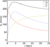 |
Fig. 1 Rotational curve of the MW. The solid black line shows the velocity of the full potential model, the dashed yellow line indicates the contribution from the halo component, the dotted blue line shows the total contribution from the discs and the dash-dotted red line the contribution from the bulge (bar and spheroid). The red symbol with error bar represents the Sun. |
3.3 Outputs
OrbIT can be customised to produce a wide variety of outputs. In its most common configuration it provides all the classical orbital parameters, the actions, and the circularity of each tracer, and it can also output a full orbital history, recording the 6D spatial information of each tracer at every timestep.
Because the underlying potential is non-static, we expect the apocentre, Rapo, and pericentre, Rperi, (and therefore the eccentricity, ecc) of the tracers to vary with time, making the physical significance of recovering of a single value for these parameters quite uncertain. To address this issue, the code computes Rapo, Rperi, and ecc for each complete orbit of each tracer, thereby producing a distribution of values. The mean and standard deviation of each distribution are then taken to be, respectively, the final output value and the corresponding uncertainty for each parameter. Quasi-periodic and more “well-behaved” tracers experience smaller variations in parameter values and therefore have small uncertainties, whereas tracers on chaotic orbits exhibit larger errors.
The actions (JR, Jθ, Jϕ) are computed following Binney & Tremaine (2008):
 (1)
(1)
 (2)
(2)
 (3)
>where L is the total angular momentum and the integral for JR is solved numerically using a composite Simpson’s 1/3 rule (Atkinson 1991).
(3)
>where L is the total angular momentum and the integral for JR is solved numerically using a composite Simpson’s 1/3 rule (Atkinson 1991).
We further exploit the calculation of the actions to compute the following quantities:
 (4)
(4)
 (5)
(5)
 (6)
(6)
These ancillary parameters allow us to explore the “projected action space map” where J∥ is the normalised z-component of the angular momentum and J⊥ gauges the relative importance of radial and vertical motions (Vasiliev 2019b; Naidu et al. 2020; Malhan et al. 2022).
The circularity, ε, is defined as the ratio of the tracer’s angular momentum to that of a maximally rotating planar orbit, which has the same specific energy as the tracer (Abadi et al. 2003; Ruchti et al. 2014; Orkney et al. 2023):
 (7)
where
(7)
where  is found by identifying the (Vc , Rc) pair that minimises the following equation for the energy of the tracer:
 (8)
where Vc is the circular velocity, defined as:
(8)
where Vc is the circular velocity, defined as:
 (9)
(9)
The full list of parameters computed with ORBIT and used throughout this work includes: Rperi, Rapo, ecc, |Zmax| (the maximum excursion from the Galactic plane), Etot, Lx, Ly, Lz, L, L⊥ (the axial, total, and perpendicular angular momenta), Jϕ, Jθ, JR, Jtot, J⊥, J∥, ε. Because of the orientation of the Galactocentric reference frame axes adopted in this work, prograde tracers have negative Lz, Jϕ, and ε, whereas retrograde tracers have positive values of these parameters.
4 Results
Recent studies on the non-conservation of the IoMs in the MW (i.e. Pagnini et al. 2023; Woudenberg & Helmi 2025; Dillamore & Sanders 2025) caused by mergers, the secular evolution of the Galaxy, the effect of the rotating bar, and several other factors, call into question the accuracy of dynamical analyses. This is the principal reason why, instead of focusing solely on the IoMs and/or adiabatic invariants, this work presents a full sample of dynamical spaces (six spaces for ten different parameters), which helps in characterising the various progenitors. For each progenitor, differences in the way the accretion event happened, its age, the mass of the accreted structure, and many other factors, result in distinct signatures across different parameter spaces. The ability to explore a vast, multidimensional parameter space is fundamental for highlighting features and trends that allow discrimination between the numerous orbital families present in our Galaxy.
The main results of our orbital analysis are summarised in Table 1, which lists the GCs studied and their most likely progenitor. Figure 2 provides an overview of the composition of the orbital families in the commonly used Lz–Etot space. Throughout this section, we highlight the main signatures in the various parameter spaces of the most important substructures in the MW and provide boundaries for the values of the dynamical parameters deemed most important for assigning a GC to a given progenitor. To determine whether a GC belongs to a particular family, we examined which “locus” it tracks across the most dynamical parameter spaces (ideally all). Here and elsewhere in the paper we define the locus of a substructure as the region of dynamical space populated by bona fide tracers belonging to it. Some parameter spaces do not explicitly allow to discriminate between prograde and retrograde tracers, but this distinction is often useful for resolving apparent overlaps between families (i.e. in Fig. 3, the green circles of retrograde GCs and the yellow circles of Helmi Streams GCs overlap, but the two families are clearly separated by their sign of Lz). In Sect. 5 we discuss the edge cases of GCs with the most uncertain associations.
4.1 Structures considered and absent progenitors
This work focuses on the following structures: the disc and bulge of the MW (making up the in-situ component), Gaia-Enceladus-Sausage (GES, Koppelman et al. 2018; Belokurov et al. 2018; Haywood et al. 2018; Helmi et al. 2018), Sagittarius (Sag, Ibata et al. 1994; Majewski et al. 2003), the Helmi Streams (HS, Helmi et al. 1999; Koppelman et al. 2019b), the retrograde halo (with a detailed discussion in Sect. 5.2), the low energy group (low-E, first labelled by Massari et al. 2019, with a detailed discussion in Sect. 5.1), Aleph (Naidu et al. 2020), Cetus (Newberg et al. 2009; Yuan et al. 2019, 2022), Typhon (Tenachi et al. 2022), and Elqui (Shipp et al. 2018, 2019).
In our analysis, we seemingly omitted some known substructures, either because the progenitor locus substantially overlaps with well-known structures or because limited data prevented us from properly identifying the progenitor. In both instances, this made it impossible to dynamically distinguish the newer candidates from well-established structures. For LMS-1/Wukong (Naidu et al. 2020; Yuan et al. 2020), the stellar component identified by Malhan et al. (2024) overlaps with the loci of the HS and GES progenitors across all parameter spaces. The loci identified for Shakti and Shiva (Malhan & Rix 2024) substantially overlap with those of the disc and low-E groups, whereas it has not been possible to produce suitable datasets to identify the loci of Icarus (Re Fiorentin et al. 2021, 2024) and Pontus (Malhan et al. 2022; Malhan 2022). In the case of Nyx (Necib et al. 2020b,a, 2022), we do not include it in our analysis due to mounting evidence that it does not represent an independent merger event (Horta et al. 2023; Wang et al. 2023).
Identification of GC progenitors based on the dynamical analysis carried out in this work.
4.2 Bulge
The MW bulge GC population is characterised by the presence of the least energetic GCs (cyan circles in Fig. 2). While all types of orbits (prograde, retrograde or radial) are possible, the value of |Lz| remains close to zero for all members of this group as they reside in the deepest part of the MW potential well. Similarly, with orbits largely confined to the bulge, these GCs occupy the bottom-left corner of Rapo − Rperi space (Fig. 3). We define bulge GCs as those with:
Etot < −1.75 × 10⁵ km2/s2
Rperi < 1.5 kpc
Rapo < 3.5 kpc.
4.3 Disc
Although there are subtle kinematical differences between the populations of tracers inhabiting the thin and thick discs of the MW, their dynamical distributions largely overlap and the two structures are better separated through chemical analysis (i.e. Bensby et al. 2014; Hayden et al. 2015). For this reason, we treat both thin- and thick-disc populations as a single structure. The MW disc is quite prominently visible in the prograde portion of the Lz−Etot space (cyan triangles in Fig. 2). Consequently, the main features of disc GCs are ε ≈ J∥ ≤ −0.5 (usually similar values, as both gauge the rotational support of an orbit) and ecc ≤ 0.6. Disc GCs are also clearly identified in the most prograde sector of the J∥ − J⊥ space (Fig. 4) and trace a characteristic sequence in the Rperi − ecc space (Fig. 5). Disc GCs generally exhibit the following defining characteristics:
−2.0 × 10⁵ km2/s2 < Etot < −1.1 × 10⁵ km2/s2
Lz < 0 kpc km/s
0.6 kpc < Rperi < 6 kpc
Ecc < 0.7
J∥/ε < −0.4.
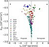 |
Fig. 2 Globular cluster sample in the angular momentum versus total energy plane. The symbols denote the affiliation to specific progenitor, as indicated in the legend: red triangles for Aleph, cyan circles for the bulge, purple triangles for Cetus, cyan triangles for the disc, yellow triangles for Elqui, red circles for Gaia-Enceladus-Sausage (GES), yellow circles for the Helmi Streams (HS), purple circles for the low energy group (low-E), green circles for the retrogrades (retro), blue circles for Sagittarius (Sag), green triangles for Typhon, and black circles for the unassociated clusters. The dashed line at Lz = 0 marks the division between prograde and retrograde sides. |
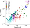 |
Fig. 3 Globular cluster sample in the apocentre versus pericentre plane, shown on a logarithmic scale. The uncertainties are computed as detailed in Sect. 3.3. The GCs are marked according to their identified progenitor, as in Fig. 2. |
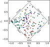 |
Fig. 4 Globular cluster sample in the parallel versus perpendicular action space. GCs with J∥ ≈ −1 are on nearly circular prograde orbits, whereas those with J∥ ≈ 1 are on nearly circular retrograde orbits. GCs with J⊥ ≈ −1 follow radial orbits while those with J⊥ ≈ 1 are on polar orbits. The GCs are marked according to their identified progenitor as in Fig. 2. |
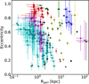 |
Fig. 5 Globular cluster sample in the pericentre versus eccentricity plane, shoqn on a semi-logarithmic scale. The uncertainties are computed as detailed in Sect. 3.3. The GCs are marked according to their identified progenitor as in Fig. 2. |
4.4 Gaia–Enceladus–Sausage (GES)
As the most massive accretion event of our Galaxy, the GES is prominently visible as a central, mildly energetic overdensity in the Lz–Etot space (red circles in Fig. 2). The population of GCs associated with this event is characterised by radial orbits (Fig. 4) with high ecc at relatively low Rperi (Fig. 5). The GES GCs are characterised by:
−1.5 × 10⁵ km2/s2 < Etot < −0.6 × 10⁵ km2/s2
Ecc > 0.7
4 kpc < Zmax < 40 kpc
−0.3 < J∥/ε < 0.3
J⊥ < 0.0.
4.5 Sagittarius (Sag)
The ongoing merger of the Sagittarius dwarf galaxy is the most recent accretion event to affect our Galaxy, and remains visible in the sky as a wide, long stellar stream. The GCs associated with the Sag event exhibit highly energetic, prograde orbits (blue circles in Fig. 2), are among those with the highest Rperi and Rapo (Fig. 3) and also have high L⊥ (Fig. 6). We define Sag GCs as those satisfying:
Etot > −0.5 × 10⁵ km2/s2
−3.0 × 10³ kpc km/s < Lz < −0.5 × 10³ kpc km/s
4.0 × 10³ kpc km/s < L⊥ < 7 × 10³ kpc km/s.
4.6 Helmi Streams (HS)
The progenitor of the Helmi Streams was among the first accreted substructures identified through the study of IoMs. The population belonging to this accretion event is characterised by prograde, high-energy orbits between the disc and the Sag populations in the Lz–Etot space (yellow circles in Fig. 2). The HS GCs also occupy a well-defined portion of the Lz − L⊥ plane (Fig. 6) and a distinctive sequence in Rperi − ecc space (Fig. 5). Our selection criteria for HS GCs are:
−1.0 × 10⁵ km2/s2 < Etot < −0.5 × 10⁵ km2/s2
Lz < −0.5 × 10³ kpc km/s
1.0 × 10³ kpc km/s < L⊥ < 4.0 × 10³ kpc km/s.
4.7 Retrogrades
The full characterisation of the retrograde portion of the halo is an ongoing effort that has seen several candidate merger events proposed over recent years. Since some of the candidate progenitors have been discarded, the consensus on others is still to be reached, and new ones continue to be proposed, we refer to Sect. 5.2 for a more in-depth discussion of each progenitor and here limit ourselves to sketching the defining traits of the retrograde family as a whole. The retrograde GCs can be clearly distinguished in Lz–L⊥ space (Fig. 6) and populate a distinctive diagonal streak of increasing ε with decreasing |Zmax| (Fig. 7). We identify as members of this group the GCs that satisfy:
Etot > −1.5 × 10⁵ km2/s2
Lz > 0.5 × 10³ kpc km/s
Zmax > 4 kpc.
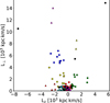 |
Fig. 6 Globular cluster sample in the vertical versus perpendicular angular momentum plane. As shown in this figure, most GCs are crowded in the low L⊥ region, where the loci of different progenitors overlap. However this space is very useful for distinguishing the various high-energy families. The GCs are marked according to their identified progenitor as in Fig. 2. |
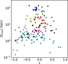 |
Fig. 7 Globular cluster sample in the circularity versus maximum vertical excursion plane, shown on a semi-logarithmic scale. The GCs are marked according to their identified progenitor as in Fig. 2. |
4.8 Low-energy group (low-E)
This group has been associated with various accretion events and in-situ structures and for the moment we retain this general label. The GCs associated with this group are characterised by energies lower than those of GES but higher than those of the bulge, and by small values of |Lz| (purple circles in Fig. 2). Similarly, GCs in the low-E group populate a region of mid ε and Zmax (Fig. 7). Low-E GCs generally exhibit the following:
−1.8 × 10⁵ km2/s2 < Etot − 1.4 × 10⁵ km2/s2
0.5 kpc < Rperi < 2 kpc
3 kpc < Rapo < 6 kpc
3 kpc < Zmax < 6 kpc
−0.5 < ε < 0.5.
4.9 Other structures
As already noted, the wealth of data that has become available over roughly the last decade has enabled the population of wider regions of the dynamical parameter spaces and has highlighted smaller confirmed and candidate merger events. The following progenitors each have only a small number of associated GCs.
4.9.1 Aleph
This structure appears to be a direct continuation of the disc at high energies and includes some of the most prograde GCs (red triangles in Fig. 2). The GCs belonging to this progenitor also exhibit higher Rperi and Rapo than their counterparts in the disc (Fig. 3). The Aleph GCs have:
Etot > −1.1 × 10⁵ km2/s2
Rperi > 5 kpc
Rapo > 10 kpc
Ecc < 0.4
Lz < −1.75 × 10³ kpc km/s.
4.9.2 Cetus
This merger, identified as a stream on a very polar orbit, is composed of prograde and very energetic tracers and lies very close to Sag in Lz–Etot space (purple triangles in Fig. 2). It is possible to distinguish genuine members of the Cetus merger for their extremely high Rperi, Rapo (Fig. 3), L⊥ (Fig. 6), and almost fully polar orbits (Fig. 4). The GCs belonging to Cetus exhibit the following:
Etot > −0.5 × 10⁵ km2/s2
Lz ≈ −2.0 × 10³ kpc km/s
L⊥ > 11.0 × 10³ kpc km/s.
4.9.3 Typhon
This is another merger discovered as a surviving stream with a long, radial orbit. We tentatively associate two high-energy GCs with this progenitor. These GCs partially overlap in some parameter spaces with the Typhon stellar populations identified by Tenachi et al. (2022) and Dodd et al. (2023) and are characterised by radial orbits (green triangles in Fig. 4) and very high Rapo coupled with very low Rperi (Fig. 3). We tentatively identify Typhon GCs as those having:
Etot > −0.7 × 10⁵ km2/s2
1.0 kpc < Rperi < 2.0 kpc
Rapo > 50 kpc
Zmax > 40 kpc.
4.9.4 Elqui
The debris stream produced by this merger is one of the most distant identified (Shipp et al. 2018, 2019). The associated GCs are retrograde and at high energies (yellow triangles in Fig. 2) but they have much higher Rperi, Rapo (Fig. 3), and L⊥ (Fig. 6) than those of the retrograde group. Being quite isolated from the rest of the retrograde family in almost all dynamical spaces, we are confident in assigning two GCs directly to Elqui. These GCs exhibit the following:
Etot > −0.5 × 10⁵ km2/s2
Lz ≈ 1.0 × 10³ kpc km/s
7.0 × 10³ kpc km/s < L⊥ < 9.0 × 10³ kpc km/s.
5 Discussion
The main difference between this work and most studies in the literature is the inclusion of the rotating bar of the MW in the model underlying the orbital integration. We tested the direct effect of including or excluding the bar by running ORBIT with and without the rotating bar and comparing the resulting outputs. The main effect of the bar is to alter the pericentres and eccentricities of GCs roughly below Etot = −1.7 × 10⁵ km2/s2 and of some clusters with highly radial orbits (i.e. very small pericentres). This translates into some changes in the classification of the GCs in the lowest-energy groups (bulge, disc, GES, and low-E), while the classification of GCs belonging to the other families is largely unaffected. Without the bar, Gran 5, NGC 6517, and NGC 6626 (all previously classified as bulge GCs), NGC 6121 (previously GES), NGC 6723 (previously unclassified), and NGC 6171 (previously disc) would instead be classified as low-E GCs. Three clusters (NGC 6256, NGC 6266, and NGC 6540) would move from the bulge to the disc family, while one (2MASS-GC02) would move from the disc to the bulge family. Finally, NGC 6284 would be classified as a GES member. These changes in the associations between GCs and progenitors make our overall classification much closer to that reported in the literature (i.e. Massari et al. 2019) because our model without a bar is essentially a variant of the widely used McMillan (2017) model.
5.1 Outliers within the groups
Although we identified defining characteristics for each family, some members stand due to their peculiar properties. In the following, we discuss these cases and the GCs contended between groups.
Starting from the bulge, it is important to mention the small number of GCs with ε and J∥ values indicative of highly counter-rotating orbits (the cyan circles at the bottom right of Fig. 7 with ε > 0.4).These GCs, VVV-CL001, Djor 2, Terzan 2, Terzan 6, Liller 1, and NGC 6325, appear clearly separated from the main bulge population due to their peculiar kinematics. Tests indicate that the spherical component of the bulge is partly responsible for their extreme kinematics. However, even when this component is removed, these GCs remain on clearly counter-rotating orbits (though less extreme). Gran 1 stands out for another reason: it is one of the least eccentric GCs in the sample, with a highly polar orbit confined to the inner bulge (topmost cyan circle at J⊥ ≈ 1.0 in Fig. 4).
At the interface between the bulge and disc groupings, there are four GCs with fairly circular orbits (cyan circles with J∥ ≥ 0.6 in Fig. 4). Despite this, NGC 6256, NGC 6266, NGC 6540, and Terzan 1 reside deep within the potential well, with very small Rapo and Rperi, and therefore we assign them to the bulge. In contrast, 2MASS-GC02 is the least energetic of the disc GCs, but its Rapo and Rperi are not small enough for it to reside in the bulge region, so we assign it to the disc family. Four of these five GCs are exactly those that move between the bulge and disc families depending on the presence or absence of the rotating bar (Sect. 5), demonstrating the influence of different choices of bulge models.
Moving on to the low-E group, it has historically been the home of tracers that could not be unambiguously attributed to either GES or the MW bulge. Several authors have linked some or all members of this group to different accretion events, namely Kraken (Kruijssen et al. 2019, 2020), Koala (Forbes 2020), and Heracles (Horta et al. 2021), which may represent the same structure. Other works have highlighted in-situ populations with similar chemo-kinematical signatures, namely Aurora (Belokurov & Kravtsov 2022; Myeong et al. 2022), Poor Old Heart (Rix et al. 2022), arguing that these structures (both accreted and in-situ) are the different facets of the same stellar population constituting the proto-Galaxy. Nevertheless, due to their tight distribution across dynamical parameter spaces, we have kept these clusters grouped together. The only two significant outliers within this family are NGC 6388 and NGC 6535, which are the most retrograde and planar low-E GCs (the rightmost purple circles in Fig. 7). Both GCs, while very retrograde, do not have sufficient energy to connect with the retrograde family or with the hypothesised Thamnos members (discussed in Sect. 5.2). Interestingly, they remain quite close in all parameter spaces, which may hint at a shared history.
The GES group of GCs contains several minor outliers. Pal 2 is among the most energetic GES GCs, exhibiting a highly radial orbit, very low Rperi, and very high Rapo (rightmost red circle in Fig. 3) and |Zmax|. However, all the other parameters identify it as a belonging to the GES progenitor. NGC 5904 and NGC 7492 are compatible with GES in most parameter spaces but have the highest L⊥ and Rperi of the family. Similarly, the high ecc and radial orbit of NGC 6584 identify it as a GES GC despite its very high |Zmax| and Rperi (these three GCs are the highest red circles in Fig. 3). NGC 6205 and NGC 7099 fit quite well within the GES family except for their uncharacteristically low ecc (red circles at ecc ≈ 0.7 in Fig. 5). Given the nature of GES as the most massive merger event of the MW, it is quite possible for its dynamical signature to be less compact than those of smaller and more recent mergers (i.e. Sag), with a modest number of outliers (six out of 26 GCs).
In the prograde and higher energy space, ESO 93-08 and Pal 10 are the two GCS with uncertain attribution to the Aleph structure (lowest red triangles in Fig. 7). Although they have a higher Etot and |Lz| than disc GCs, they have much lower |Zmax| and L⊥ than the other members of Aleph and may instead be the outermost disc GCs. Given the uncertainty in the nature and characteristics of the Aleph progenitor, it remains unclear whether these GCs are more closely linked to the disc.
NGC 4590, NGC 5824, and NGC 6426 are the GCs on the most prograde circular orbits within the HS family (yellow circles with J∥ < −0.5 in Fig. 4), similar to disc GCs, but with Rapo, Zmax, and L⊥ values consistent with the HS group and lying on the HS sequence in Rperi − ecc space. The presence of debris on prograde orbits is expected from a merger generally believed to be prograde (even if not planar) and relatively massive at the time of accretion (Helmi et al. 1999).
The Sag group is well isolated across all parameter spaces with only Eridanus being slightly an outlier due to its higher |Zmax|.
5.2 The retrograde family
The retrograde halo has been populated by several candidate progenitors over the years, starting with Sequoia (Myeong et al. 2018; Barbá et al. 2019; Matsuno et al. 2019; Myeong et al. 2019) and Elqui (Shipp et al. 2018, 2019) to several more. Studies based on simulations of the complex dynamics of galactic mergers suggest that high mass-ratio events spread their debris across large portions of parameter space, spilling copiously in the retrograde portion of the halo, and causing these debris to be mistaken for independent mergers (Koppelman et al. 2020; Amarante et al. 2022; Khoperskov et al. 2023). Arjuna (proposed by Naidu et al. 2020) has been rejected for this very reason and its sibling I’itoi (from the same work) is under similar scrutiny, hampered by a dearth of chemical information (Naidu et al. 2021; Horta et al. 2023).
Thamnos (Koppelman et al. 2019a) is another candidate member of the retrograde family, first identified as a pair of overdensities very close to each other in the mid-energy, retrograde portion of the Lz–Etot space. Koppelman et al. (2019a) and subsequent works estimated a very low mass for the Thamnos progenitor (MThamnos ≤ 5 · 107 M⊙), making it very unlikely that it would harbour any GC capable of surviving the merger while retaining a recognisable dynamical signature to the present time. Moreover, recent work on the chemical characterisation of substructures seems to indicate that the stellar population of Thamnos is heavily contaminated by in-situ and GES tracers (i.e. Fig. 15 from Ruiz-Lara et al. 2022). Nevertheless, based on a purely dynamical analysis, several clusters unassociated with other progenitors or within the retrograde family fall in or near the loci identified by the Thamnos stellar component in the various dynamical spaces. NGC 5139 (also known as ωCen) and FSR 1758 are the GCs that most closely track the Thamnos stellar population across all parameter spaces while Gran 2 exhibits a slightly out-of-plane, more polar orbit (with higher |Zmax| and L⊥). The aforementioned NGC 6388 and NGC 6535 exhibit retrograde planar orbits very similar to those of the Thamnos tracers, however they reside much deeper in the MW potential well and have lower Etot, Rapo, and Rperi.
Antaeus/L-RL64 is an extremely retrograde and highly energetic merger remnant identified by Oria et al. (2022) and Ruiz-Lara et al. (2022). More recently, the small structure of ED-3 has been identified in the retrograde halo (Dodd et al. 2023), occupying loci that are connected or contiguous to Antaeus/L-RL64 in all parameter spaces. The association between the two structures has been corroborated by the findings of Ceccarelli et al. (2024). Based on their strongly retrograde orbits, NGC 3201 and NGC 6101 could be associated with this structure. Although the two clusters do not directly track the stars identified as Antaeus members by Oria et al. (2022) and Dodd et al. (2022), NGC 3201 closely follows the loci of ED-3 members across all dynamical spaces, allowing us to establish a tentative association between these two GCs and the Antaeus progenitor.
5.3 Unclassified GCs
Some MW GCs share some defining characteristics with the aforementioned groups but appear strongly discordant in other parameter spaces. We briefly review these outliers that cannot be unequivocally assigned to any progenitor.
AM-4 lies amid the retrograde group in Lz–Etot space but has a much higher Rperi and much lower ecc that distinguish it as a clear extreme outsider within this family. Crater is too extreme in all parameter spaces to be a part of any retrograde family. Sagittarius II is Crater’s counterpart in the prograde portion of dynamical space, being a distant outlier from all identified groups. NGC 6934 is too energetic for, and has a higher Rapo than, Helmi Streams GCs but has Rperi and |Zmax| too low for Sag GCs, and its orbit is too radial for both families. Located between the loci of the low-E and GES families, NGC 6284 has Rapo, Rperi, and |Zmax| value that are too high to belong to the former group and ecc that is too low, together with a more polar than radial orbit, to be classified as a GES GC. BH 140 and Djor 1 have many characteristics of disc GCs, with prograde and circular orbits, but their Rapo, Rperi, and ecc values are too high compared to the other disc GCs. The orbit of NGC 5897 is not circular enough for it to be a (thick) disc GC and not radial enough to belong to the GES. Similarly, its Rapo, Rperi, and |Zmax| values are too high for the disc population and its ecc is too low for the GES. Gran 3 has a retrograde circular orbit with a very low ecc, which distinguishes it from nearby identified groups at similar energies. NGC 6723 likewise has a very low ecc (making its membership in the low-E group very unlikely) and is characterised by a peculiar, extremely polar orbit.
5.4 Literature comparison
Reviewing some recent literature on the classification of the MW GC population, we do not compare directly our work with that of Bica et al. (2024), as their selection is based on ages and chemistry, whereas ours relied solely on dynamical information. Similarly, the selection presented by Belokurov & Kravtsov (2024), while incorporating some dynamical information, is guided and calibrated using the [Al/Fe] abundance ratio and only distinguishes between the in-situ and accreted components. Nevertheless, we find general agreement with the classification by Belokurov & Kravtsov (2024), with the notable exception of the low-E family, whose members the authors mostly classify as in-situ (likely attributing them to the Aurora population, Belokurov & Kravtsov 2022). For the families identified in both studies, we also find general agreement with Chen & Gnedin (2024), again with the notable exception of the low-E group, identified as in-situ by these authors. Our results agree closely with the classification of high- and mid-energy GCs by Callingham et al. (2022); Sun et al. (2023); Massari (2025), but differs for the lowest-energy groups (bulge, disc, and low-E). All these studies use as an underlying model the static potential from McMillan (2017), and it is clear that discrepancies in the classification of the least energetic GCs arise from the impact of the rotating bar on the orbital parameters. In the case of Massari (2025) it is worth also noting that part of the differences are due to these authors not including Aleph in their list of progenitors, whereas we slightly unpacked their “high energy” group into some known progenitors (and Typhon). We note several differences with respect to the classification by Malhan et al. (2022) primarily due to their adoption of a partially different set of progenitors, namely LMS-1/Wukong, Pontus, and an unknown retrograde merger (see Sect. 4.1 for our reasons for excluding these progenitors). One of the first studies to employ an underlying potential including a rotating bar is Pérez-Villegas et al. (2020), however they use a different classification (bulge, disc, inner halo, and outer halo) and without distinguishing between the various merger events. Nevertheless our lists of bulge and disc clusters closely agree, with minor discrepancies due to the different ecc threshold used to define disc membership. Another study incorporating a rotating bar into the underlying potential is Garro et al. (2023), which focuses on a small subsample of clusters. Our results are in broad agreement with theirs, with orbital parameters consistent within the errors.
6 Conclusions
We present OrbIT, a new in-house tool for precise and efficient orbit integration to study galactic dynamics. The code’s novelty resides in fully accounting for a time-varying potential at all stages, especially for the recovery of the orbital parameters and their associated uncertainties. OrbIT, with its up-to-date potential model of the MW including the rotating bar and a spherical bulge component, has already been used to characterise the RR Lyrae population of the bulge (Olivares Carvajal et al. 2024). In this work, we used ORBIT to study the dynamics of the galactic GCs and to classify them among the various families of merger events.
Using information derived from six different dynamical parameter spaces (orbital parameters, IoMs, and adiabatic invariants), we provide a full dynamical characterisation of the in-situ population and different progenitors. Including the rotating bar changes the associations of low-energy GCs, while our comprehensive dynamical analysis enables clear associations for a number of previously unassociated high-energy GCs to specific structures (four GCs to Aleph and two each to Cetus, Typhon, Elqui and Antaeus). We also propose the association of three GCs to the Thamnos progenitor, further complicating the conundrum posed by this very small, old merger.
Several GCs remain of ambiguous ancestry or are clear outliers within their families, and some still lack any associated progenitor. This work represents a step towards complete characterisation of the MW inventory, and our purely dynamical view must be complemented with cutting-edge chronochemical studies (i.e. the CARMA project, Massari et al. 2023; Aguado-Agelet et al. 2025; Ceccarelli et al. 2025).
In future work, we will explore the effect of the rotating bar in more depth, including both its direct gravitational pull affecting the central region of the MW and the resonances it generates as a time-varying component of the potential.
Data availability
The data underlying this article come from public sources listed in Section 2. The full table C.1 is available at the CDS via https://cdsarc.cds.unistra.fr/viz-bin/cat/J/A+A/706/A130 (an excerpt of the table is provided in Appendix C).
Acknowledgements
The authors would like to thank the anonymous referee for insightful comments that helped improve and clarify the manuscript. Thanks also go to D. Massari, E. Ceccarelli, M. Bellazzini, A. Mucciarelli and E. Dodd for valuable discussions. MDL acknowledges financial support from the National Agency for Research and Development (ANID), Millenium Science Initiative, ICN12_009 and from the project “LEGO – Reconstructing the building blocks of the Galaxy by chemical tagging” (PI: Mucciarelli) granted by the Italian MUR through contract PRIN2022LLP8TK_001. MZ acknowledges support by the National Agency for Research and Development (ANID) Millenium Science Initiative, ICN12_009 and AIM23-0001, awarded to the Millennium Institute of Astrophysics (MAS) and the ANID BASAL Center for Astrophysics and Associated Technologies (CATA) through grant FB210003, and from ANID FONDECYT Regular No. 1230731. BA-T acknowledges support from the ANID Doctoral Fellowship through grant number 21231305. FG gratefully acknowledges support from the French National Research Agency (ANR) funded projects “MWDisc” (ANR-20-CE31-0004) and “Pristine” (ANR-18-CE31-0017). This research made use of the Astropy (Astropy Collaboration 2013, 2018), Matplotlib (Hunter 2007) and Numpy (Harris et al. 2020) packages.
References
- Abadi, M. G., Navarro, J. F., Steinmetz, M., & Eke, V. R. 2003, ApJ, 597, 21 [NASA ADS] [CrossRef] [Google Scholar]
- Aguado-Agelet, F., Massari, D., Monelli, M., et al. 2025, A&A, 704, A255 [NASA ADS] [CrossRef] [EDP Sciences] [Google Scholar]
- Amarante, J. A. S., Debattista, V. P., Beraldo e Silva, L., Laporte, C. F. P., & Deg, N. 2022, ApJ, 937, 12 [NASA ADS] [CrossRef] [Google Scholar]
- Astropy Collaboration (Robitaille, T. P., et al.) 2013, A&A, 558, A33 [NASA ADS] [CrossRef] [EDP Sciences] [Google Scholar]
- Astropy Collaboration (Price-Whelan, A. M., et al.) 2018, AJ, 156, 123 [Google Scholar]
- Atkinson, K. E. 1991, An Introduction to Numerical Analysis, 2nd edn. (John Wiley & Sons) [Google Scholar]
- Bacon, R., Accardo, M., Adjali, L., et al. 2010, SPIE Conf. Ser., 7735, 773508 [Google Scholar]
- Barbá, R. H., Minniti, D., Geisler, D., et al. 2019, ApJ, 870, L24 [CrossRef] [Google Scholar]
- Baumgardt, H. 2017, MNRAS, 464, 2174 [Google Scholar]
- Baumgardt, H., & Hilker, M. 2018, MNRAS, 478, 1520 [Google Scholar]
- Baumgardt, H., & Vasiliev, E. 2021, MNRAS, 505, 5957 [NASA ADS] [CrossRef] [Google Scholar]
- Belokurov, V., & Kravtsov, A. 2022, MNRAS, 514, 689 [NASA ADS] [CrossRef] [Google Scholar]
- Belokurov, V., & Kravtsov, A. 2024, MNRAS, 528, 3198 [CrossRef] [Google Scholar]
- Belokurov, V., Erkal, D., Evans, N. W., Koposov, S. E., & Deason, A. J. 2018, MNRAS, 478, 611 [Google Scholar]
- Bennett, M., & Bovy, J. 2019, MNRAS, 482, 1417 [NASA ADS] [CrossRef] [Google Scholar]
- Bensby, T., Feltzing, S., & Oey, M. S. 2014, A&A, 562, A71 [NASA ADS] [CrossRef] [EDP Sciences] [Google Scholar]
- Bica, E., Ortolani, S., Barbuy, B., & Oliveira, R. A. P. 2024, A&A, 687, A201 [NASA ADS] [CrossRef] [EDP Sciences] [Google Scholar]
- Binney, J., & Tremaine, S. 2008, Galactic Dynamics, 2nd edn. (Princeton University Press) [Google Scholar]
- Bovy, J. 2015, ApJS, 216, 29 [NASA ADS] [CrossRef] [Google Scholar]
- Bullock, J. S., & Johnston, K. V. 2005, ApJ, 635, 931 [Google Scholar]
- Callingham, T. M., Cautun, M., Deason, A. J., et al. 2022, MNRAS, 513, 4107 [NASA ADS] [CrossRef] [Google Scholar]
- Ceccarelli, E., Massari, D., Mucciarelli, A., et al. 2024, A&A, 684, A37 [NASA ADS] [CrossRef] [EDP Sciences] [Google Scholar]
- Ceccarelli, E., Massari, D., Aguado-Agelet, F., et al. 2025, A&A, accepted [arXiv:2503.02939] [Google Scholar]
- Chandrasekhar, S. 1943a, ApJ, 97, 255 [Google Scholar]
- Chandrasekhar, S. 1943b, ApJ, 97, 263 [NASA ADS] [CrossRef] [Google Scholar]
- Chandrasekhar, S. 1943c, ApJ, 98, 54 [NASA ADS] [CrossRef] [Google Scholar]
- Chen, Y., & Gnedin, O. Y. 2024, Open J. Astrophys., 7, 23 [NASA ADS] [Google Scholar]
- Chiba, R., & Schönrich, R. 2021, MNRAS, 505, 2412 [NASA ADS] [CrossRef] [Google Scholar]
- Chiba, R., Friske, J. K. S., & Schönrich, R. 2021, MNRAS, 500, 4710 [Google Scholar]
- Dillamore, A. M., & Sanders, J. L. 2025, MNRAS, 542, 1331 [Google Scholar]
- Dillamore, A. M., Belokurov, V., & Evans, N. W. 2024, MNRAS, 532, 4389 [NASA ADS] [CrossRef] [Google Scholar]
- Dodd, E., Callingham, T. M., Helmi, A., et al. 2022, VizieR Online Data Catalog: Gaia DR3 of substructure in the stellar halo (Dodd+, 2023), VizieR On-line Data Catalog: J/A+A/670/L2. Originally published in: 2023A & A…670L…2D [Google Scholar]
- Dodd, E., Callingham, T. M., Helmi, A., et al. 2023, A&A, 670, L2 [NASA ADS] [CrossRef] [EDP Sciences] [Google Scholar]
- Eggen, O. J., Lynden-Bell, D., & Sandage, A. R. 1962, ApJ, 136, 748 [NASA ADS] [CrossRef] [Google Scholar]
- Forbes, D. A. 2020, MNRAS, 493, 847 [Google Scholar]
- Forbes, D. A., & Bridges, T. 2010, MNRAS, 404, 1203 [NASA ADS] [Google Scholar]
- Gaia Collaboration (Prusti, T., et al.) 2016, A&A, 595, A1 [NASA ADS] [CrossRef] [EDP Sciences] [Google Scholar]
- Gaia Collaboration (Vallenari, A., et al.) 2023, A&A, 674, A1 [NASA ADS] [CrossRef] [EDP Sciences] [Google Scholar]
- Garro, E. R., Minniti, D., Alessi, B., et al. 2022, A&A, 659, A155 [NASA ADS] [CrossRef] [EDP Sciences] [Google Scholar]
- Garro, E. R., Fernández-Trincado, J. G., Minniti, D., et al. 2023, A&A, 669, A136 [NASA ADS] [CrossRef] [EDP Sciences] [Google Scholar]
- Gómez, F. A., Helmi, A., Brown, A. G. A., & Li, Y.-S. 2010, MNRAS, 408, 935 [Google Scholar]
- Gran, F., Zoccali, M., Saviane, I., et al. 2022, MNRAS, 509, 4962 [Google Scholar]
- Gran, F., Kordopatis, G., Zoccali, M., et al. 2024, A&A, 683, A167 [NASA ADS] [CrossRef] [EDP Sciences] [Google Scholar]
- GRAVITY Collaboration (Abuter, R., et al.) 2019, A&A, 625, L10 [NASA ADS] [CrossRef] [EDP Sciences] [Google Scholar]
- Hairer, E., Lubich, C., & Wanner, G. 2003, Acta Numerica, 12, 399 [NASA ADS] [CrossRef] [Google Scholar]
- Harris, C. R., Millman, K. J., van der Walt, S. J., et al. 2020, Nature, 585, 357 [NASA ADS] [CrossRef] [Google Scholar]
- Hartke, J., Kakkad, D., Reyes, C., et al. 2020, SPIE Conf. Ser., 11448, 114480V [NASA ADS] [Google Scholar]
- Hayden, M. R., Bovy, J., Holtzman, J. A., et al. 2015, ApJ, 808, 132 [Google Scholar]
- Haywood, M., Di Matteo, P., Lehnert, M. D., et al. 2018, ApJ, 863, 113 [Google Scholar]
- Haywood, M., Khoperskov, S., Cerqui, V., et al. 2024, A&A, 690, A147 [NASA ADS] [CrossRef] [EDP Sciences] [Google Scholar]
- Helmi, A., & de Zeeuw, P. T. 2000, MNRAS, 319, 657 [Google Scholar]
- Helmi, A., & White, S. D. M. 1999, MNRAS, 307, 495 [CrossRef] [Google Scholar]
- Helmi, A., White, S. D. M., de Zeeuw, P. T., & Zhao, H. 1999, Nature, 402, 53 [Google Scholar]
- Helmi, A., Babusiaux, C., Koppelman, H. H., et al. 2018, Nature, 563, 85 [Google Scholar]
- Horta, D., Schiavon, R. P., Mackereth, J. T., et al. 2021, MNRAS, 500, 1385 [Google Scholar]
- Horta, D., Schiavon, R. P., Mackereth, J. T., et al. 2023, MNRAS, 520, 5671 [NASA ADS] [CrossRef] [Google Scholar]
- Hunter, J. D. 2007, Comput. Sci. Eng., 9, 90 [NASA ADS] [CrossRef] [Google Scholar]
- Ibata, R. A., Gilmore, G., & Irwin, M. J. 1994, Nature, 370, 194 [Google Scholar]
- Khoperskov, S., Minchev, I., Libeskind, N., et al. 2023, A&A, 677, A90 [NASA ADS] [CrossRef] [EDP Sciences] [Google Scholar]
- Koppelman, H., Helmi, A., & Veljanoski, J. 2018, ApJ, 860, L11 [NASA ADS] [CrossRef] [Google Scholar]
- Koppelman, H. H., Helmi, A., Massari, D., Price-Whelan, A. M., & Starkenburg, T. K. 2019a, A&A, 631, L9 [NASA ADS] [CrossRef] [EDP Sciences] [Google Scholar]
- Koppelman, H. H., Helmi, A., Massari, D., Roelenga, S., & Bastian, U. 2019b, A&A, 625, A5 [NASA ADS] [CrossRef] [EDP Sciences] [Google Scholar]
- Koppelman, H. H., Bos, R. O. Y., & Helmi, A. 2020, A&A, 642, L18 [NASA ADS] [CrossRef] [EDP Sciences] [Google Scholar]
- Kruijssen, J. M. D., Pfeffer, J. L., Reina-Campos, M., Crain, R. A., & Bastian, N. 2019, MNRAS, 486, 3180 [Google Scholar]
- Kruijssen, J. M. D., Pfeffer, J. L., Chevance, M., et al. 2020, MNRAS, 498, 2472 [NASA ADS] [CrossRef] [Google Scholar]
- Leaman, R., VandenBerg, D. A., & Mendel, J. T. 2013, MNRAS, 436, 122 [Google Scholar]
- Lian, J., Zasowski, G., Mackereth, T., et al. 2022, MNRAS, 513, 4130 [NASA ADS] [CrossRef] [Google Scholar]
- Lim, D., Koch-Hansen, A. J., Chung, C., et al. 2021, A&A, 647, A34 [NASA ADS] [CrossRef] [EDP Sciences] [Google Scholar]
- Long, K., & Murali, C. 1992, ApJ, 397, 44 [NASA ADS] [CrossRef] [Google Scholar]
- Lövdal, S. S., Ruiz-Lara, T., Koppelman, H. H., et al. 2022, A&A, 665, A57 [NASA ADS] [CrossRef] [EDP Sciences] [Google Scholar]
- Mace, G., Sokal, K., Lee, J.-J., et al. 2018, SPIE Conf. Ser., 10702, 107020Q [NASA ADS] [Google Scholar]
- Majewski, S. R., Skrutskie, M. F., Weinberg, M. D., & Ostheimer, J. C. 2003, ApJ, 599, 1082 [NASA ADS] [CrossRef] [Google Scholar]
- Majewski, S. R., Schiavon, R. P., Frinchaboy, P. M., et al. 2017, AJ, 154, 94 [NASA ADS] [CrossRef] [Google Scholar]
- Malhan, K. 2022, ApJ, 930, L9 Malhan, K., & Rix, H.-W. 2024, ApJ, 964, 104 [Google Scholar]
- Malhan, K., Ibata, R. A., Sharma, S., et al. 2022, ApJ, 926, 107 [NASA ADS] [CrossRef] [Google Scholar]
- Malhan, K., Yuan, Z., Ibata, R. A., et al. 2024, VizieR Online Data Catalog: Stars of the LMS-1 stream with sp. obs. (Malhan+, 2021), VizieR On-line Data Catalog: J/ApJ/920/51. Originally published in: 2021ApJ…920…51M [Google Scholar]
- Marín-Franch, A., Aparicio, A., Piotto, G., et al. 2009, ApJ, 694, 1498 [Google Scholar]
- Massari, D. 2025, RNAAS, 9, 64 [Google Scholar]
- Massari, D., Koppelman, H. H., & Helmi, A. 2019, A&A, 630, L4 [NASA ADS] [CrossRef] [EDP Sciences] [Google Scholar]
- Massari, D., Aguado-Agelet, F., Monelli, M., et al. 2023, A&A, 680, A20 [NASA ADS] [CrossRef] [EDP Sciences] [Google Scholar]
- Matsuno, T., Aoki, W., & Suda, T. 2019, ApJ, 874, L35 [NASA ADS] [CrossRef] [Google Scholar]
- McKee, C. F., Parravano, A., & Hollenbach, D. J. 2015, ApJ, 814, 13 [Google Scholar]
- McMillan, P. J. 2017, MNRAS, 465, 76 [NASA ADS] [CrossRef] [Google Scholar]
- Minniti, D., Lucas, P. W., Emerson, J. P., et al. 2010, New A, 15, 433 [Google Scholar]
- Minniti, D., Fernández-Trincado, J. G., Smith, L. C., et al. 2021, A&A, 648, A86 [NASA ADS] [CrossRef] [EDP Sciences] [Google Scholar]
- Minniti, D., Matsunaga, N., Fernández-Trincado, J. G., et al. 2024, A&A, 683, A150 [NASA ADS] [CrossRef] [EDP Sciences] [Google Scholar]
- Miyamoto, M., & Nagai, R. 1975, PASJ, 27, 533 [NASA ADS] [Google Scholar]
- Moni Bidin, C., Mauro, F., Geisler, D., et al. 2011, A&A, 535, A33 [NASA ADS] [CrossRef] [EDP Sciences] [Google Scholar]
- Moreno, E., Fernández-Trincado, J. G., Pérez-Villegas, A., Chaves-Velasquez, L., & Schuster, W. J. 2022, MNRAS, 510, 5945 [NASA ADS] [CrossRef] [Google Scholar]
- Myeong, G. C., Evans, N. W., Belokurov, V., Sanders, J. L., & Koposov, S. E. 2018, MNRAS, 478, 5449 [NASA ADS] [CrossRef] [Google Scholar]
- Myeong, G. C., Vasiliev, E., Iorio, G., Evans, N. W., & Belokurov, V. 2019, MNRAS, 488, 1235 [Google Scholar]
- Myeong, G. C., Belokurov, V., Aguado, D. S., et al. 2022, ApJ, 938, 21 [NASA ADS] [CrossRef] [Google Scholar]
- Naidu, R. P., Conroy, C., Bonaca, A., et al. 2020, ApJ, 901, 48 [Google Scholar]
- Naidu, R. P., Conroy, C., Bonaca, A., et al. 2021, ApJ, 923, 92 [NASA ADS] [CrossRef] [Google Scholar]
- Navarro, J. F., Frenk, C. S., & White, S. D. M. 1996, ApJ, 462, 563 [Google Scholar]
- Necib, L., Ostdiek, B., Lisanti, M., et al. 2020a, ApJ, 903, 25 [NASA ADS] [CrossRef] [Google Scholar]
- Necib, L., Ostdiek, B., Lisanti, M., et al. 2020b, Nat. Astron., 4, 1078 [NASA ADS] [CrossRef] [Google Scholar]
- Necib, L., Ostdiek, B., Lisanti, M., et al. 2022, Nat. Astron., 6, 866 [Google Scholar]
- Newberg, H. J., Yanny, B., & Willett, B. A. 2009, ApJ, 700, L61 [NASA ADS] [CrossRef] [Google Scholar]
- Olivares Carvajal, J., Zoccali, M., Rojas-Arriagada, A., et al. 2022, MNRAS, 513, 3993 [NASA ADS] [CrossRef] [Google Scholar]
- Olivares Carvajal, J., Zoccali, M., De Leo, M., et al. 2024, A&A, 687, A312 [NASA ADS] [CrossRef] [EDP Sciences] [Google Scholar]
- Oria, P.-A., Tenachi, W., Ibata, R., et al. 2022, ApJ, 936, L3 [NASA ADS] [CrossRef] [Google Scholar]
- Orkney, M. D. A., Laporte, C. F. P., Grand, R. J. J., et al. 2023, MNRAS, 525, 683 [NASA ADS] [CrossRef] [Google Scholar]
- Pagnini, G., Di Matteo, P., Khoperskov, S., et al. 2023, A&A, 673, A86 [NASA ADS] [CrossRef] [EDP Sciences] [Google Scholar]
- Park, C., Jaffe, D. T., Yuk, I.-S., et al. 2014, SPIE Conf. Ser., 9147, 91471D [NASA ADS] [Google Scholar]
- Peebles, P. J. E. 1965, ApJ, 142, 1317 [NASA ADS] [CrossRef] [Google Scholar]
- Peebles, P. J. E., & Yu, J. T. 1970, ApJ, 162, 815 [NASA ADS] [CrossRef] [Google Scholar]
- Pérez-Villegas, A., Barbuy, B., Kerber, L. O., et al. 2020, MNRAS, 491, 3251 [Google Scholar]
- Plummer, H. C. 1911, MNRAS, 71, 460 [Google Scholar]
- Prudil, Z., Kunder, A., Beraldo e Silva, L., et al. 2025, A&A, 695, A211 [NASA ADS] [CrossRef] [EDP Sciences] [Google Scholar]
- Queiroz, A. B. A., Chiappini, C., Perez-Villegas, A., et al. 2021, A&A, 656, A156 [NASA ADS] [CrossRef] [EDP Sciences] [Google Scholar]
- Re Fiorentin, P., Spagna, A., Lattanzi, M. G., & Cignoni, M. 2021, ApJ, 907, L16 [NASA ADS] [CrossRef] [Google Scholar]
- Re Fiorentin, P., Spagna, A., Lattanzi, M. G., Cignoni, M., & Vitali, S. 2024, ApJ, 977, 278 [NASA ADS] [CrossRef] [Google Scholar]
- Read, J. I., Pontzen, A. P., & Viel, M. 2006, MNRAS, 371, 885 [NASA ADS] [CrossRef] [Google Scholar]
- Reid, M. J. 2008, in IAU Symposium, Vol. 248, A Giant Step: from Milli- to Micro-arcsecond Astrometry, eds. W. J. Jin, I. Platais, & M. A. C. Perryman, 141 [Google Scholar]
- Rix, H.-W., Chandra, V., Andrae, R., et al. 2022, ApJ, 941, 45 [NASA ADS] [CrossRef] [Google Scholar]
- Roberts, J. A. G., & Quispel, G. R. W. 1992, Phys. Rep., 216, 63 [Google Scholar]
- Ruchti, G. R., Read, J. I., Feltzing, S., Pipino, A., & Bensby, T. 2014, MNRAS, 444, 515 [Google Scholar]
- Ruiz-Lara, T., Matsuno, T., Lövdal, S. S., et al. 2022, A&A, 665, A58 [NASA ADS] [CrossRef] [EDP Sciences] [Google Scholar]
- Saito, R. K., Hempel, M., Minniti, D., et al. 2012, A&A, 537, A107 [NASA ADS] [CrossRef] [EDP Sciences] [Google Scholar]
- Sanders, J. L., Smith, L., & Evans, N. W. 2019, MNRAS, 488, 4552 [NASA ADS] [CrossRef] [Google Scholar]
- Schönrich, R., Binney, J., & Dehnen, W. 2010, MNRAS, 403, 1829 [NASA ADS] [CrossRef] [Google Scholar]
- Searle, L., & Zinn, R. 1978, ApJ, 225, 357 [Google Scholar]
- Shen, J., & Zheng, X.-W. 2020, Res. Astron. Astrophys., 20, 159 [CrossRef] [Google Scholar]
- Shipp, N., Drlica-Wagner, A., Balbinot, E., et al. 2018, ApJ, 862, 114 [Google Scholar]
- Shipp, N., Li, T. S., Pace, A. B., et al. 2019, ApJ, 885, 3 [NASA ADS] [CrossRef] [Google Scholar]
- Ströbele, S., La Penna, P., Arsenault, R., et al. 2012, SPIE Conf. Ser., 8447, 844737 [Google Scholar]
- Stuik, R., Bacon, R., Conzelmann, R., et al. 2006, New A Rev., 49, 618 [Google Scholar]
- Sun, G., Wang, Y., Liu, C., et al. 2023, Res. Astron. Astrophys., 23, 015013 [CrossRef] [Google Scholar]
- Tenachi, W., Oria, P.-A., Ibata, R., et al. 2022, ApJ, 935, L22 [NASA ADS] [CrossRef] [Google Scholar]
- Trick, W. H. 2022, MNRAS, 509, 844 [Google Scholar]
- Valenti, E., Zoccali, M., Gonzalez, O. A., et al. 2016, A&A, 587, L6 [NASA ADS] [CrossRef] [EDP Sciences] [Google Scholar]
- Vasiliev, E. 2019a, MNRAS, 482, 1525 [Google Scholar]
- Vasiliev, E. 2019b, MNRAS, 484, 2832 [Google Scholar]
- Vasiliev, E., & Baumgardt, H. 2021, MNRAS, 505, 5978 [NASA ADS] [CrossRef] [Google Scholar]
- Verlet, L. 1967, Phys. Rev., 159, 98 [CrossRef] [Google Scholar]
- Wang, S., Necib, L., Ji, A. P., et al. 2023, ApJ, 955, 129 [NASA ADS] [CrossRef] [Google Scholar]
- Wegg, C., Gerhard, O., & Portail, M. 2015, MNRAS, 450, 4050 [NASA ADS] [CrossRef] [Google Scholar]
- White, S. D. M., & Rees, M. J. 1978, MNRAS, 183, 341 [Google Scholar]
- Woudenberg, H. C., & Helmi, A. 2025, A&A, 700, A240 [NASA ADS] [CrossRef] [EDP Sciences] [Google Scholar]
- Yuan, Z., Smith, M. C., Xue, X.-X., et al. 2019, ApJ, 881, 164 [NASA ADS] [CrossRef] [Google Scholar]
- Yuan, Z., Chang, J., Beers, T. C., & Huang, Y. 2020, ApJ, 898, L37 [Google Scholar]
- Yuan, Z., Malhan, K., Sestito, F., et al. 2022, ApJ, 930, 103 [NASA ADS] [CrossRef] [Google Scholar]
- Zinn, R. 1985, ApJ, 293, 424 [Google Scholar]
- Zinn, R. 1996, in Astronomical Society of the Pacific Conference Series, 92, Formation of the Galactic Halo…Inside and Out, eds. H. L. Morrison & A. Sarajedini, 211 [Google Scholar]
- Zoccali, M., Valenti, E., & Gonzalez, O. A. 2018, A&A, 618, A147 [NASA ADS] [CrossRef] [EDP Sciences] [Google Scholar]
- Zoccali, M., Quezada, C., Contreras Ramos, R., et al. 2024, A&A, 689, A240 [NASA ADS] [CrossRef] [EDP Sciences] [Google Scholar]
Appendix A Impact of observational errors: worst cases
As mentioned in Sect. 2, we tested that our results (the attribution of each GC to a specific progenitor) are robust even when taking into account observational errors. Here we show the worst cases out of the entire sample, even for them the classification doesn’t become ambiguous when taking into account the uncertainties. In Fig. A.1 we show the high energy GCs AM 1 (grey star), Eridanus (blue star), Palomar 3 (red star) and Palomar 4 (orange star), the GCs with the highest distance uncertainties, in the Lz − L⊥ space. The underlying coloured contours in the same tonalities (greys for AM 1, blues for Eridanus, etc…) show the density distribution of 1000 integrations with different input phase space values generated by extracting from the error distributions of each GC. We also show the nearest progenitor families (Sag, HS, the retrogrades, and the other Elqui member). It is clear from the figure that, even for the cases with the largest scatter (AM 1, Palomar 4), accounting for the errors doesn’t change the classification of these GCs. Similarly, in Fig. A.2 we show 2MASS-GC01 (red star) and Patchick 122 (green star), the GCs with the highest uncertainties on their velocity vector, in ε − Zmax space. The underlying matching coloured contours show the density distribution of 1000 iterations accounting for the observational errors. As before, we also show the nearest progenitor families (bulge, disc, and low-E) and it appears clear that, even accounting for the errors, the two GCs cannot be identified as anything but disc GCs.
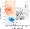 |
Fig. A.1 Lz − L⊥ space distribution of the GCs with the highest distance uncertainties (filled stars). The underlying matching coloured contours are the distributions of 1000 iterations accounting for the observational errors. The other filled symbols (circles, triangles) are the GCs members of the nearby progenitor families. |
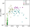 |
Fig. A.2 ε − Zmax space distribution of the GCs with the highest velocity vector uncertainties (filled stars). The underlying matching coloured contours are the distributions of 1000 iterations accounting for the observational errors. The other filled symbols (circles, triangles) are the GCs members of the nearby progenitor families. |
Appendix B Sanity checks and tests of ORBIT
To ensure that ORBIT works properly we performed an extensive array of tests, both in configurations with a symmetric and static potential (excluding the rotating bar and the central BH) and with the full time-evolving model. In the static and symmetric case, we checked the conservation of the 2 IoMs, the total mechanical energy Etot = K +U and the angular momentum around the symmetry axis, Lz. With the full model, the only surviving IoM is the Jacoby energy (or Jacobi integral Binney & Tremaine 2008), EJ = Etot − Ωb · L (where Ωb is the pattern speed of the rotation and L is the angular momentum corresponding to the axis of rotation, in our case Lz). Fig. B.1 shows the ratios of the variation of the three IoMs during integrations of 5 · 106 steps for a total of 5 Gyr. The ratios are computed as ∆X/X0 with the variation of each IoM being the value at every step minus the initial value, ∆X = X − X0 (with X being one of Etot, Lz, EJ).
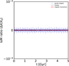 |
Fig. B.1 Evolution of the IoMs over a typical orbital integration. In black and red, respectively, the total mechanical energy Etot and the angular momentum Lz for the case with a symmetric and static potential. In blue the Jacoby integral EJ for the case with the full potential. |
Appendix C Data table
Table C.1 is an excerpt of the results derived by ORBIT, the full table is only available in electronic form at the CDS.
Recovered orbital parameters, IoMs, adiabatic invariants, and derived quantities used for this analysis for each GC studied. The full table is available at the CDS.
All Tables
Identification of GC progenitors based on the dynamical analysis carried out in this work.
Recovered orbital parameters, IoMs, adiabatic invariants, and derived quantities used for this analysis for each GC studied. The full table is available at the CDS.
All Figures
|
Fig. 1 Rotational curve of the MW. The solid black line shows the velocity of the full potential model, the dashed yellow line indicates the contribution from the halo component, the dotted blue line shows the total contribution from the discs and the dash-dotted red line the contribution from the bulge (bar and spheroid). The red symbol with error bar represents the Sun. |
| In the text | |
|
Fig. 2 Globular cluster sample in the angular momentum versus total energy plane. The symbols denote the affiliation to specific progenitor, as indicated in the legend: red triangles for Aleph, cyan circles for the bulge, purple triangles for Cetus, cyan triangles for the disc, yellow triangles for Elqui, red circles for Gaia-Enceladus-Sausage (GES), yellow circles for the Helmi Streams (HS), purple circles for the low energy group (low-E), green circles for the retrogrades (retro), blue circles for Sagittarius (Sag), green triangles for Typhon, and black circles for the unassociated clusters. The dashed line at Lz = 0 marks the division between prograde and retrograde sides. |
| In the text | |
|
Fig. 3 Globular cluster sample in the apocentre versus pericentre plane, shown on a logarithmic scale. The uncertainties are computed as detailed in Sect. 3.3. The GCs are marked according to their identified progenitor, as in Fig. 2. |
| In the text | |
|
Fig. 4 Globular cluster sample in the parallel versus perpendicular action space. GCs with J∥ ≈ −1 are on nearly circular prograde orbits, whereas those with J∥ ≈ 1 are on nearly circular retrograde orbits. GCs with J⊥ ≈ −1 follow radial orbits while those with J⊥ ≈ 1 are on polar orbits. The GCs are marked according to their identified progenitor as in Fig. 2. |
| In the text | |
|
Fig. 5 Globular cluster sample in the pericentre versus eccentricity plane, shoqn on a semi-logarithmic scale. The uncertainties are computed as detailed in Sect. 3.3. The GCs are marked according to their identified progenitor as in Fig. 2. |
| In the text | |
|
Fig. 6 Globular cluster sample in the vertical versus perpendicular angular momentum plane. As shown in this figure, most GCs are crowded in the low L⊥ region, where the loci of different progenitors overlap. However this space is very useful for distinguishing the various high-energy families. The GCs are marked according to their identified progenitor as in Fig. 2. |
| In the text | |
|
Fig. 7 Globular cluster sample in the circularity versus maximum vertical excursion plane, shown on a semi-logarithmic scale. The GCs are marked according to their identified progenitor as in Fig. 2. |
| In the text | |
|
Fig. A.1 Lz − L⊥ space distribution of the GCs with the highest distance uncertainties (filled stars). The underlying matching coloured contours are the distributions of 1000 iterations accounting for the observational errors. The other filled symbols (circles, triangles) are the GCs members of the nearby progenitor families. |
| In the text | |
|
Fig. A.2 ε − Zmax space distribution of the GCs with the highest velocity vector uncertainties (filled stars). The underlying matching coloured contours are the distributions of 1000 iterations accounting for the observational errors. The other filled symbols (circles, triangles) are the GCs members of the nearby progenitor families. |
| In the text | |
|
Fig. B.1 Evolution of the IoMs over a typical orbital integration. In black and red, respectively, the total mechanical energy Etot and the angular momentum Lz for the case with a symmetric and static potential. In blue the Jacoby integral EJ for the case with the full potential. |
| In the text | |
Current usage metrics show cumulative count of Article Views (full-text article views including HTML views, PDF and ePub downloads, according to the available data) and Abstracts Views on Vision4Press platform.
Data correspond to usage on the plateform after 2015. The current usage metrics is available 48-96 hours after online publication and is updated daily on week days.
Initial download of the metrics may take a while.