| Issue |
A&A
Volume 706, February 2026
|
|
|---|---|---|
| Article Number | A215 | |
| Number of page(s) | 14 | |
| Section | Astrophysical processes | |
| DOI | https://doi.org/10.1051/0004-6361/202557116 | |
| Published online | 10 February 2026 | |
Multi-wavelength emission in resistive pulsar magnetospheres
Université de Strasbourg, CNRS, Observatoire astronomique de Strasbourg, UMR 7550 F-67000 Strasbourg, France
★ Corresponding author: This email address is being protected from spambots. You need JavaScript enabled to view it.
Received:
5
September
2025
Accepted:
10
December
2025
Abstract
Context. Neutron star magnetospheres are well described in the two extreme cases of a vacuum field and a plasma-filled force-free regime. However, neither of these descriptions allows for magnetic field dissipation into particle kinetic energy and thus high-energy radiation. Some physical processes must be invoked to produce observational signatures typical of pulsars.
Aims. In this paper, we compute a full set of neutron star magnetosphere structures from the basic vacuum regime to the dissipation-less force-free regime by implementing a resistive prescription for the plasma. A comparison to the radiation reaction limit is also discussed. We investigated the impact of these resistive magnetospheres on the multi-wavelength emission properties based on the polar cap model for radio wavelengths, the slot gap model for X-rays, and the striped wind model for γ-rays.
Methods. We performed time-dependent pseudo-spectral simulations of the full Maxwell equations including a resistive Ohm’s law. We deduced the polar cap shape and size, the Poynting flux, the magnetic field structure, and the current sheet surface, depending on magnetic obliquity χ and conductivity σ.
Results. We found that the geometry of the magnetosphere close to the stellar surface is not impacted by the amount of resistivity. Polar cap rims remain very similar in shape and size. However, the Poynting flux varies significantly, as well as the magnetic field sweep-back in the vicinity of the light cylinder. This bending of field lines reflects in the γ-ray pulse profiles, changing the γ-ray peak separation Δ as well as the time lag δ between the radio pulse and γ-ray peaks. X-ray pulse profiles are also drastically affected by resistivity.
Conclusions. A full set of multi-wavelength light curves can be compiled for future comparison with the third γ-ray pulsar catalogue. This systematic study will help constrain the amount of magnetic energy that flows into particle kinetic energy and is shared by radiation.
Key words: magnetic fields / plasmas / radiation mechanisms: general / pulsars: general / gamma rays: general / X-rays: general
© The Authors 2026
 Open Access article, published by EDP Sciences, under the terms of the Creative Commons Attribution License (https://creativecommons.org/licenses/by/4.0), which permits unrestricted use, distribution, and reproduction in any medium, provided the original work is properly cited.
This article is published in open access under the Subscribe to Open model. This email address is being protected from spambots. You need JavaScript enabled to view it. to support open access publication.
1. Introduction
Pulsars are detected across a broad band of the electromagnetic spectrum, from radio wavelengths up to very high-energy photons in the GeV or TeV range. More than 300 γ-ray pulsars are known today (Smith et al. 2023), for a total of about 4.400 radio pulsars listed in the online Australia Telescope National Facility (ATNF) pulsar catalogue1 (Manchester et al. 2005). Because this emission is pulsed, it must be produced close to the neutron star surface, in its magnetosphere and within its wind. Photons are produced by accelerating charged particles to ultra-relativistic speeds in the neutron star’s ultra-strong electromagnetic field. However, the details of this acceleration and radiation processes are still poorly understood. The location of the emission sites is also loosely constrained. A quantitative understanding of pulsar machinery requires a self-consistent modelling of the magnetosphere coupled to its emission mechanisms. Radiation implies that the star cannot be simply surrounded by empty space as in the Deutsch vacuum field solution (Deutsch 1955). In the opposite limit, the magnetosphere cannot contain an ideal plasma with infinite conductivity, zero pressure, and zero inertia, as the resulting force-free regime prohibits dissipation in such a regime. The truth lies between these two regimes: the magnetosphere must contain a plasma in a non-ideal regime that converts the star’s rotational kinetic energy into high-frequency electromagnetic radiation, in addition to the low-frequency, large-amplitude electromagnetic waves launched by the rotating dipole.
Whereas neutron star global electrodynamics is now well reproduced thanks to numerical force-free simulations using finite-difference schemes (Spitkovsky 2006) or pseudo-spectral algorithms (Pétri 2012; Cao et al. 2016b), the outcome in terms of realistic pulsed emission remains unclear. This has led several authors to consider resistive or dissipative magnetospheres in order to localise the sites where the energy transfer to particles and radiation occurs (Li et al. 2012; Palenzuela 2013; Cao et al. 2016a; Kalapotharakos et al. 2014; Kato 2017; Cao & Yang 2020; Pétri 2020b, 2022). The most detailed picture is, however, given by kinetic simulations such as particle-in-cell (PIC) codes, reaching close to force-free conditions as in Philippov et al. (2015), Cerutti et al. (2015) or reaching close to vacuum conditions as in Mottez (2024). Most of these studies (Bai & Spitkovsky 2010; Kalapotharakos et al. 2012a; Brambilla et al. 2015; Cerutti et al. 2016b; Kalapotharakos et al. 2017; Cao & Yang 2019; Yang & Cao 2021; Cao & Yang 2022; Barnard et al. 2022; Kalapotharakos et al. 2023; Cao et al. 2024) have focused on high-energy emission because, at least for γ-ray pulsars, a high fraction of the spin-down luminosity flows into γ-ray photons. However, a multi-wavelength modelling effort, combining radio, X-ray, and γ-ray knowledge, has emerged (Pétri 2024; Yang & Cao 2024) as a powerful tool to further constrain emission sites. Polarisation is another important measurable quantity for constraining the geometry of the radiative sources within the magnetosphere (Cerutti et al. 2016a; Pétri & Mitra 2021).
Particle acceleration and high-energy radiation production depend strongly on the plasma regime within the magnetosphere because the magnetic field-aligned electric field strongly couples to the plasma screening efficiency. However, the exact plasma regime remains a matter of debate, especially as it can vary from place to place. Pair creation via photon disintegration in a strong magnetic field or via photon-photon interaction largely controls this regime, as shown in PIC simulations (Chen & Beloborodov 2014; Chen et al. 2020). The observational outcome of these various regimes should lead to different unambiguous imprints detectable in their multi-wavelength light curves.
The aim of this paper is, in a first step, to compute force-free, radiative, and resistive pulsar magnetospheres in the same framework, using the same pseudo-spectral numerical algorithm to compare the similarities and discrepancies between these assumptions. In a second step, we extract the observational signature by computing the multi-wavelength light curves from radio to γ rays, assuming a polar cap model for radio, a slot gap model for non-thermal X-rays, and a striped wind model for the γ rays. We stress that our emission models are solely based on geometrical considerations related to the magnetic field structure, ignoring the physical mechanisms behind the radiation processes. Sect. 2 presents the different regimes used to construct pulsar magnetospheres. Sect. 3 discusses the magnetospheric solutions found in the different regimes. The derived multi-wavelength emission properties are summarised in Sect. 4. Conclusions are drawn in Sect. 5.
2. Magnetospheric plasma model
The vacuum and force-free dipole magnetospheres represent the two extreme models of a simple neutron star environment. The real magnetosphere lies somewhere in between these two limits, allowing for magnetic reconnection and dissipation. These non-ideal effects are described in their simplest form by a conductivity summarised in a single scalar parameter denoted by σ. In this section, after a brief review of neutron star magnetospheric structure and emission sites, we recall the electric current prescription for the force-free, radiative, and resistive plasma regimes; the vacuum current vanishing identically.
2.1. Review on magnetospheric structure and emission
Let us first briefly recall the qualitative structure of the magnetosphere and its related emission sites (see Pétri 2016; Cerutti & Beloborodov 2017; Philippov & Kramer 2022 for recent reviews on their structure and dynamics, and Harding 2017 for their emission models). The neutron star surface magnetic field is assumed to be dipolar and dragged by the stellar rotation, leading to regions of open and closed field lines. In the closed region, within the force-free regime, inside the light cylinder of radius rL, the plasma co-rotates with the star, and field lines remain inside rL. The open region corresponds to magnetic field lines crossing the light cylinder and reaching very large distances. The surface separating the closed region from the open region is called the separatrix (Kalapotharakos et al. 2012b). Inside the light cylinder, the northern part of this separatrix joins the southern part at the so-called Y-point exactly at the light cylinder. The structure of this Y-point remains under debate as it could in fact be a T-point (see for instance Contopoulos et al. 2024 for an illustration).
Based on this magnetospheric structure, three distinct regions were identified as potential emission sites for radio photons, X-rays, and γ rays. First, the polar cap is expected to produce the radio pulses; next, the slot gap for non-thermal X-rays (Pétri et al. 2024); and the current sheet within the striped wind for γ rays (Pétri 2011). Pétri (2024) details these three emission models, for which even general-relativistic effects have been included by Pétri (2018). Figure 1 sketches the emission sites and the magnetosphere topology for a general oblique rotator.
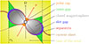 |
Fig. 1. Schematic view of the pulsar magnetosphere, showing the separatrix and the emission sites. |
2.2. Maxwell equations
In all subsequent models, the plasma inertia and pressure are neglected. The plasma only furnishes the required charge ρe and current j densities to evolve Maxwell equations, written in standard Systéme International (SI) units as
 (1a)
(1a)
 (1b)
(1b)
 (1c)
(1c)
 (1d)
(1d)
Here, ε0 is the vacuum permittivity, μ0 the vacuum permeability, and c the speed of light. Apart from the boundary conditions on the stellar surface and at infinity where outgoing wave conditions are imposed, the current density j represents the only unknown of the problem. Once fixed according to a given plasma model, Maxwell equations are solved numerically, leading to a solution for the magnetosphere. So, let us describe the simplest possibilities for this electric current density j. We consider three current prescriptions requiring either no free parameter, as in the force-free approximation, or only one parameter: the pair multiplicity κ for the radiative model or a conductivity parameter σ for the resistive model.
2.3. Current prescription
2.3.1. Force-free regime
The vacuum case is trivial, with j = 0 leading to the exact analytical solution given by Deutsch (1955). In the exact opposite limit, an ideal plasma with infinite conductivity according to σ = +∞ leads to the force-free prescription where the current density becomes (Gruzinov 1999; Blandford 2002)
 (2)
(2)
This current produces no work on particles since j ⋅ E = 0 because E ⋅ B = 0 by construction. All the rotational kinetic energy goes into the Poynting flux of the low-frequency large-amplitude electromagnetic wave. For completeness and faithful comparisons with other plasma regimes shown in this paper, we compute some force-free magnetosphere solutions with exactly the same numerical setup.
2.3.2. Radiative approximation
By transitioning to a weakly dissipative regime, we define the electric current associated with the radiation reaction limit velocity field. The detailed derivation is provided by Pétri (2016), and the associated radiative current density j, under minimal assumptions, is explained in Pétri (2020b). The final expression simplifies to
 (3)
(3)
where κ is the pair multiplicity factor that governs dissipation. This current transforms the Poynting flux energy into particle kinetic energy because j ⋅ E > 0 and, subsequently, into multi-wavelength high-energy radiation, primarily in X-rays and γ rays. The electric and magnetic field strengths, E0 and |B0|, respectively, are related to the electromagnetic invariants2 by E0 B0 = E ⋅ B and E02 − c2 B0 = E2 − c2 B2. Physically, E0 and |B0| represent the strength of the electric and magnetic field in any frame in which they are parallel. However, in a series of previous studies (Pétri 2020a,b, 2022), we found that the dissipation remains weak except along the separatrix and around the Y-point. The low dissipation rate occurs because the plasma is always at least partially filled with the charge density ρe imposed by the Maxwell-Gauss law Eq. (1c) combined with a non-negligible parallel current given by the second term in Eq. (3), which never vanishes because |ρe| (1 + 2 κ)≥|ρe|. As already demonstrated in these aforementioned studies (Pétri 2020a,b, 2022), this approximation is nearly indistinguishable from the force-free regime.
2.3.3. Resistive model
To address this limitation of the radiative current, we attempted another prescription that allows for a vanishing parallel current if σ → 0. The derivation of this current is provided by Li et al. (2012) and given by
 (4)
(4)
with
 (5)
(5)
The previous factor |ρe| (1 + 2 κ) in Eq. (3) is now replaced by Γ σ E0/c in Eq. (4). As shown in the next section, the limit σ → 0 corresponds to the vacuum solution, whereas the σ → +∞ limit corresponds to the force-free regime. Therefore, σ can be interpreted as a type of conductivity controlling the rate of magnetic dissipation into plasma heating and acceleration – a process not captured by these models. We emphasise that Eq. (4) is a special case, called the minimal velocity limit, of a more general expression derived by Li et al. (2012), which includes a velocity component of the fluid v∥ along the common direction of E0 and B0. However, imposing v∥ ≠ 0 does not guarantee that the vacuum case is approached whenever σ → 0, and, therefore, σ can no longer be interpreted as a conductivity if v∥ ≠ 0. If the limiting case v∥ = ±c is applied to the general prescription of the current density in Li et al. (2012), it reduces to a formal expression very similar to Eq. (3), with no dependence on the conductivity σ. For instance, imposing v∥ = −sign(ρe) c, corresponding to the instantaneous acceleration to the speed of light in the direction of the co-moving electric field (see Eq. (30) in Pétri 2020a), leads exactly to Eq. (3) with κ = 0.
3. Magnetospheric solutions
In this section, we present the numerical results of resistive and radiative magnetosphere solutions obtained by our pseudo-spectral time evolution code, using spherical polar coordinates (r, θ, φ) (see Pétri 2012 for details of implementation and Pétri 2014 for its extension to general relativity). To gain more insight into these results, we first show the spin-down luminosity as a function of the obliquity and plasma regime, then the magnetic field structure, and finally the polar cap shapes and the separatrix. This serves as the basis for the discussion of the multi-wavelength emission properties of resistive magnetospheres. For numerical purposes, we set the inner boundary of the simulation domain to R1/rL = 0.2 and the outer boundary to R2/rL = 8, where rL = c/Ω is the light-cylinder radius and Ω the neutron star angular velocity. The numerical grid size is Nr × Nθ × Nφ = 129 × 32 × 64. The simulations ran on a single-CPU machine and took one week on average. The value R1 corresponds to the neutron star radius R. The most dissipative radiative case is given by κ = 0 and is the only radiative model considered in this work. The case κ = 0 means that no pairs are created and the plasma is fully charge-separated; only primary particles contribute to the current and charge densities. Dissipation of the electromagnetic wave is the largest in this case. However, this regime is still far from vacuum as particles populate the entire magnetosphere and mimic an almost force-free regime. For the conductivity σ, we chose values such that it smoothly transitions between the vacuum and force-free case, taking log(σ/ε0 Ω) = {−1, 0, 1, 2, 3}. The normalised conductivity parameter is defined by  . The obliquity of the pulsar was chosen to be χ = {0° ,15° ,30° ,45° ,60° ,75° ,90° }.
3.1. Spin down luminosity
The fundamental quantity controlling the secular evolution of the neutron star magnetosphere is its spin-down, the rate of energy radiated by the electromagnetic wave. As a reference value, we computed the luminosity through the Poynting flux for a perpendicular point dipole rotating in vacuum, given by Deutsch (1955)
 (6)
(6)
where B is the magnetic field strength at the equator of a spherical star, Ω is its rotation rate, and R is its radius. Expression (6) is valid for a point dipole or in the limit R ≪ rL. If R ≲ rL, then some corrections including spherical Hankel functions must be applied; see Pétri (2015), particularly Eq. (46).
Fig. 2 shows the spin-down luminosity L as a function of the magnetic obliquity χ and the plasma regime: VAC for the vacuum, FFE for the force-free, RAD for the radiative regime with κ = 0, and RES for the resistive plasma with the value of  in parentheses. As expected, for a given obliquity, all luminosities vary between the vacuum and the force-free cases: the vacuum is reached for
  , whereas the force-free regime corresponds to the limit
  . All solutions show a sin2χ dependence with respect to obliquity χ. The results can be summarised by the expression
 (7)
(7)
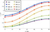 |
Fig. 2. Spin-down luminosity as a function of obliquity χ of the magnetosphere. The vacuum (VAC) and force-free (FFE) cases are shown as references. |
with the value of the coefficients a and b given in Table 1. Note that in the vacuum case, a = 0, but b ≲ 1 because of the large ratio R/rL = 0.2, leading to a leading-order correction of this factor b by an amount b ≈ 1 − (R/rL)2 ≈ 0.96.
Fig. 3 shows the same results but from a different perspective, changing the plasma regime and fixing the obliquity χ. The transition from the VAC to the FFE solution is clearly seen. The heuristic parameter σ helps control the plasma regime from non-dissipation to maximally dissipation conditions, even though it hides all the complex microphysics of particle dynamics and radiation – which can only be captured by performing detailed kinetic simulations.
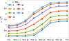 |
Fig. 3. Spin-down luminosity for fixed obliquity χ of the magnetosphere. The vacuum (VAC) and force-free (FFE) cases are shown as limiting cases. |
3.2. Particle versus Poynting luminosity
The luminosity computed in our model takes only the Poynting flux into account. There is no contribution from the particles in either the force-free limit or the resistive regime because the particles have zero inertia. They only contribute to charge and current densities. Therefore, strictly speaking they do not take away any energy from the neutron star. However, because of their mass, number density, and relativistic speed, a particle kinetic energy flux in fact exists which amounts to approximately
 (8)
(8)
assuming a particle number density depending on the Goldreich-Julian charge-separated density (of the order of 2 ε0 Ω B), a pair multiplicity factor κ, and a bulk Lorentz factor Γ for the cold wind. We neglect the contribution from the hot current sheet (see for instance Pétri 2019). This energy flux remains negligible as long as the ratio
 (9)
(9)
remains much smaller than unity. This ratio is shown in Fig. 4 for Γ = 10 (mildly relativistic flow) and κ = 0 (no pair creation, fully charge-separated plasma current) for the γ-ray pulsars in the third catalogue 3PC (Smith et al. 2023), separately for millisecond pulsars (MSPs) and young pulsars (YPs). This ratio is always smaller than 10−7; thus even for typical values for the bulk flow Lorentz factor of Γ ≲ 100 and pair multiplicity of κ ≲ 105, this ratio remains smaller than one. The energy carried away by the particle represents at most several percent of the Poynting flux.
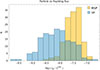 |
Fig. 4. Ratio Lp/L⊥vac for Γ = 10 and κ = 0 for MSPs and YPs, according to data from 3PC. |
3.3. Magnetic field
The resistivity significantly impacts the geometry of the magnetic field at large distances from the neutron star surface. The vacuum and force-free field lines are very different at the light cylinder, as seen in Fig. 5 for a perpendicular rotator. All other possible geometries between these two limiting cases are found depending on the conductivity σ. The presence of a plasma within the magnetosphere forces the field lines to sweep backwards more strongly than in the vacuum regime. For instance, the field line rooting at the magnetic pole crosses the light cylinder at a later rotational phase when σ increases, reaching the point where it joins the force-free limit. As a consequence, the curvature of the field lines also increases because of the plasma back reaction. As the γ-ray emission is expected to be produced in the vicinity of the light cylinder, this sweep back has a profound impact on the radio to γ-ray time lag as observed in the third pulsar catalogue (3PC), (Smith et al. 2023). We discuss this in depth in Section 4. The RAD results are very similar to the FFE results and therefore not shown for readability reasons.
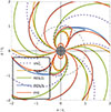 |
Fig. 5. Magnetic field lines in the equatorial plane of an orthogonal rotator for different plasma regimes going from VAC to FFE through RES. The dashed circle depicts the light-cylinder radius, and the grey disk the neutron star. |
The separatrix represents an important surface within the magnetosphere. It is significantly impacted by plasma resistivity. Fig. 6 shows a cross-section in the μ − Ω plane, i.e. the plane defined by the magnetic moment vector μ and the rotation axis Ω, for an obliquity χ = 45° and for different values of the conductivity σ. An increase in this conductivity shrinks the volume of the separatrix. We note that the location where this separatrix touches the light cylinder does not significantly depend on the plasma regime. This is an important point since these places are the base of the current sheet in the striped wind. The low-altitude region of the separatrix also delimits the radio beam opening angle, and recent studies (Pétri et al. 2024) suggest that non-thermal X-ray emission is supported by this surface. Therefore, the separatrix is at the heart of the multi-wavelength pulsed emission of pulsars.
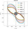 |
Fig. 6. Separatrix cross-section in the μ − Ω plane for an obliquity χ = 45° and different plasma regimes. The vertical dashed lines depict the light cylinder, while the grey disk represents the neutron star. |
3.4. Polar caps
The structure of the wind and its current sheet rely on the shape of the separatrix rooted to the polar cap geometry. It is therefore important to localise on the neutron star surface the feet of the last closed field lines, which separate the inert co-rotating closed magnetosphere from the out-flowing plasma responsible for radio and high-energy emission. We therefore computed the polar cap rims in the resistive regime for any obliquity and conductivity. Results for χ = {15° ,45° ,75° } are shown in Fig. 7. The vacuum rotator produces the smallest size polar caps, whereas the force-free regime produces mainly the largest caps. For high inclinations, the vacuum case produces artificial cusps in the polar caps that disappear in a plasma-loaded magnetosphere. In this regime, all the polar cap rims tend to circularise independently of the obliquity.
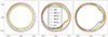 |
Fig. 7. Polar cap shape viewed from above for χ = {15° ,45° ,75° }, from left to right. The vacuum case is shown in dashed black lines. |
The shapes found correspond to an artificially large neutron star radius with R/rL = 0.2. This limitation is due to the computational resources needed to compute magnetosphere solutions with smaller stellar radii. However, we checked that the polar cap rims previously shown in Fig. 7 scale with the theoretical ratio  for R/rL ≪ 1. To verify this assertion, we plot the polar cap rims in the extreme vacuum limit with dashed lines and the resistive polar caps and force-free polar caps with solid lines in Fig. 8 for different values of the ratio R/rL = {0.1, 0.2, 0.3}. For smaller ratios, the agreement is even better, as can be checked accurately in the vacuum case for any R/rL (for which analytical solutions exist).
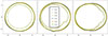 |
Fig. 8. Polar cap shapes for different obliquities χ = {15° ,45° ,75° }, from left to right, and several ratios R/rL = {0.1, 0.2, 0.3}. The sizes are normalised according to the scaling with respect to |


Moreover, in the force-free regime, to very good accuracy, the polar cap rim is insensitive to the obliquity χ, as shown in Fig. 9. It is accurately approximated by a constant radius rpc independent of χ such that
 (10)
(10)
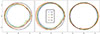 |
Fig. 9. Polar cap rim centred onto the magnetic pole for different inclination angles χ in the vacuum (left), resistive (middle), and force-free regime (right). The fit to Eq. (10) is shown as a dashed black circle of normalised radius 1.2. |
This relation can serve as a good proxy for estimating the size of polar caps deduced from the dipolar magnetic field.
4. Multi-wavelength pulsed emission
The above considerations described the magnetic environment of the neutron star and its magnetic topology, focusing on important concepts such as spin-down luminosity, polar caps, and separatrix surface. However, such configurations are not easily deduced by direct measurements. We must rely on indirect inference by observing their pulsed electromagnetic emission. Therefore, in this section, we investigate in detail the multi-wavelength outcome of this magnetospheric structure, starting with radio emission, then the geometry at the base of the current sheet and its related γ-ray radiation, and finally the X-ray emission properties. Curvature along the separatrix and central magnetic field line plays an important role in photon energy and is also computed. Finally, as a direct application to existing observations, we computed multi-wavelength light curves and extracted the radio time lag variation with respect to the γ-ray peak separation for immediate comparison with 3PC.
More specifically, for the radio pulses, we assumed curvature emission along the open magnetic field lines delimited by the polar cap rim. Emission occurs at an altitude of R/rL = 0.2. For X-rays, curvature emission occurs only along the separatrix, starting at an altitude above the radio emission site and stopping before reaching the light cylinder. These inner and outer boundaries can vary but are prescribed by the user. Finally, for γ rays, synchrotron emission is expected within the current sheet of the striped wind, in the radial direction.
4.1. Radio pulse profile and width
Pulsars are mostly detected at low frequencies in the radio waveband. The radio pulse profile exhibits a complex structure, which is usually frequency-dependent. The pulse width W is related to the pulsar geometry χ and observer viewing angle ζ as a function of the radio beam half-opening angle ρ such that (Gil et al. 1984)
 (11)
(11)
This expression relies on the static dipole approximation for the radio beam geometry, seen as a perfect cone. In a more realistic context, magnetic sweep-back and magnetospheric currents should be taken into account, as in the sweep-back shown in Fig. 5. Fig. 10 shows sky maps of regions illuminated by the radio beam, depending on the emission height s above the stellar surface and on the magnetospheric regime (from top to bottom: vacuum, resistive, and force-free). The magnetic dipole moment inclination is fixed to χ = 60° and the emission height normalised to the light-cylinder radius, as given in the legend by the ratio s/rL.
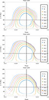 |
Fig. 10. Pulse width for the radio pulse profile for χ = 60°, depending on the regime. From top to bottom: Vacuum, resistive, and force-free. The emission height along the field lines, starting from the surface, is given by s and normalised with respect to the light-cylinder radius, s/rL. |
In the vacuum case, we retrieve a cusp shape reminiscent of the polar cap rim. This spike disappears in the FFE regime. Note that due to the relatively large R/rL ratio, the pulse width remains rather large, with a duty cycle of 20%–30%. Decreasing this ratio R/rL diminishes the pulse width accordingly, following expression (10). An important point to notice is that large pulse widths do not necessarily imply an almost aligned rotator. Indeed, for low obliquities such as χ = 30° −45° and emission heights of s/rL ≈ 0.5, we still observe cases with a radio pulse spanning 90% of the period, depending on the viewing angle ζ. Consequently, the MSPs detected with high radio duty cycles are compatible with mild obliquities and emission height values reaching a significant fraction of the light-cylinder radius.
As a comparison, we show in Fig. 11 the emission pattern expected from the static dipole (solid lines) in connection with the pulsar width given in Eq. (11). Neither aberration nor retardation effects are included because we simply follow the dipole field lines, computing the local tangent t to these lines and assuming photons are emitted at a position marked by the spherical angles (θe, φe). This leads to the following components for the tangent vector t (see Pétri 2024 for its derivation):
 (12a)
(12a)
 (12b)
(12b)
 (12c)
(12c)
 (12d)
(12d)
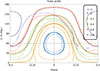 |
Fig. 11. Sky map for the radio pulse profile at χ = 60°: static dipole (dashed lines, without the 1.2 correction factor, solid lines with the 1.2 correction factor) and a force-free dipole (dotted lines). |
The viewing angle is therefore ζ = arccos(tz/t), and the azimuth is φ = arctan(tx, ty). Qualitatively, the shape resembles the force-free one; however, in the latter case, aberration, retardation, and magnetic field sweep-back break the east-west symmetry. We emphasise that the above expression (12a) also applies to the X-ray pulse profile because both radio and X-rays rely on the separatrix surface, which has a simple analytical expression for the static dipole. Fig. 11 also shows a comparison between the pulse profiles expected from the force-free magnetosphere (dotted lines) and from the static dipole (dashed lines). For the force-free simulations, we set R/rL = 0.1. At low altitude s = 0 corresponding to the surface of the star, both profiles look similar except for a larger size in the force-free case, by a factor of around 1.2 (see Eq. (10)). For increasing emission heights, the force-free pulse is shifted to earlier phases due to magnetic sweep-back; however, the overall width remains within a factor of 1.2 of the vacuum case. Correcting for the phase shift, both regimes qualitatively look very similar at any height. However, if the factor of 1.2 is included in the vacuum polar cap shape, discrepancies arise at a height of s/rL ≳ 0.6.
4.2. Current sheet and γ-ray sky map
In the striped wind model (Bogovalov 1999; Kirk et al. 2002), γ rays are essentially produced within the current sheet outside the light cylinder (Pétri 2011; Mochol 2017). This surface determines the properties of the light curves, including pulse shape, morphology, and phase lag with respect to the radio pulse, among others. In order to understand the impact of the resistivity onto the current sheet geometry, we show examples of this surface by plotting a 3D view of this current sheet, as shown in Fig. 12 for χ = 45° in the vacuum (blue), resistive (green), and FFE (red) magnetosphere.
 |
Fig. 12. 3D view of the current sheet geometry for the vacuum (blue), resistive (green) and FFE (red) magnetosphere. |
Fig. 13 shows a complete set of γ-ray sky maps overlapped with the radio pulse profile for several inclinations χ = {15° ,45° ,75° }. In the force-free regime, the peak emission follows the split monopole pattern given by
 |
Fig. 13. γ-ray sky maps for several inclinations χ = {15° ,45° ,75° }, from top to bottom. For completeness, the radio pulse profile is also shown. The conductivity increases from left to right, starting with the vacuum case and ending with the FFE regime. The solid blue lines indicate the sky maps deduced from a static dipole for the radio profile, and the solid cyan lines indicate the sky maps deduced from the split monopole solution Eq. (13). |
 (13)
(13)
See appendix A for the derivation of this relation. The angle φ0 allows for a possible phase shift in the light curve. In the present work, it was set to φ0 ≈ −0.09. This curve is plotted in green lines in Fig. 13. We indeed see good agreement between this relation and the FFE simulations. Moving to the vacuum regime, the γ-ray peak shifts to earlier phases, and the range of significant emission in the ζ direction also increases. This is related to the geometry of the current sheet, which opens up wider in vacuum compared to FFE (see Fig. 12). Emission disappears at low and high latitudes, ζ ≲ 30° and ζ ≳ 150°, because in our model γ-ray photons are emitted only outside the light cylinder. This is a purely geometric effect mostly insensitive to the obliquity χ.
4.3. X-rays sky map
The same exercise was repeated for the non-thermal X-ray produced along the separatrix. Results are shown in Fig. 14 and overlapped with the radio pulse profile. If the X-ray pulse profiles are phase-aligned with the radio pulse, decreasing the conductivity shifts the X-ray pulses to later phases. This behaviour is opposite to expectations for the γ-ray light curve. The variations in pulse shape are drastic in X-rays. Indeed, whereas in the FFE case the peak in X-ray lags the radio pulse, in low conductivity and vacuum regimes this X-ray peak leads the radio profile. See for instance Fig. 19 for a typical example of peak changing in X-rays.
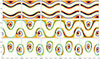 |
Fig. 14. Same as Fig. 13, but for the X-ray sky maps. The solid blue lines indicate the sky maps deduced from a static dipole for the radio profile, and the cyan lines for the X-ray profile. |
As a consequence, the most visible impact of the magnetosphere resistivity resides in shaping the non-thermal X-ray emission and not the radio and/or γ-ray energy band. The X-ray sky maps suppose that photons emanate from the separatrix. In this particular example, emission begins at R/rL = 0.2 and stops at R/rL = 0.3. Other emission heights are possible and may lead to different X-ray sky maps (see for instance Pétri 2024 for additional examples).
4.4. Curvature along the magnetic axis and the separatrix
Photons within the magnetosphere are produced via synchrotron and curvature radiation. The typical synchrotron energy is imposed by the local magnetic field strength, whereas the curvature energy depends linearly on the local curvature of the magnetic field lines. In this section, we are interested in the latter radiation mechanism. Two types of field lines are particularly important: magnetic field lines sustaining the separatrix and those along the magnetic axis.
Fig. 15 shows the curvature κc in units of 1/rL for several plasma regimes when sliding along the magnetic axis. In all cases, the curvature increases from the surface to an altitude of R/rL ≈ 0.5 − 1 and then decreases. The FFE regime offers the highest curvature, which is expected since the electric current bends the field lines more strongly than in the vacuum or resistive cases. If radio photons are produced by curvature radiation along field lines around the magnetic axis, we expect to observe low frequencies at low altitudes and high frequencies at high altitudes – the exact opposite of the radius-to-frequency mapping (RFM) findings (Komesaroff 1970). This frequency evolution with altitude, and thus with curvature, relies on the fact that all emitting particles possess the same Lorentz factor γ (i.e. a mono-energetic particle distribution function), irrespective of their height above the polar cap or along the magnetic axis, because the typical curvature radiation frequency is given by ωcurv ≈ (3/2) γ3 c κc. From this expression, we immediately notice that an increase in curvature κc leads to a similar increase in frequency ωcurv. The associated angle between the magnetic axis and the tangent to the central magnetic field line is shown in Fig. 16. It is largest in the FFE case and diminishes in the resistive and vacuum cases. In the vacuum case, the central field line remains almost straight up to the light cylinder, where it deviates by less than 20°. This contrasts with the line in the FFE case, which deviates by more than 60°.
 |
Fig. 15. Curvature along the central magnetic field line for vacuum, resistive, and FFE with obliquity χ = 60°. |
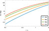 |
Fig. 16. Angles between the magnetic axes and the central magnetic field lines for vacuum, resistive, and FFE with obliquity χ = 60°. |
In the separatrix region, the situation reverses. Fig. 17 indeed shows the curvature κc in units of 1/rL for several plasma regimes when sliding along field lines, starting at the surface of the star close to the north pole, reaching a maximal distance when grazing the light cylinder, and returning to the stellar surface at the south pole. During this back and forth travel, two lines appear for the same radial coordinate r: one for the leading direction (forward motion) and the other for the receding direction (backward motion). In all cases, the curvature decreases from the surface to an altitude of R/rL ≈ 0.5, then increases again up to the point where the magnetic field line returns to the surface. The configuration is not symmetric with respect to the turning point, as seen in the plot. Moreover, the FFE regime offers the highest curvature, which is expected since the electric current bends the field lines more strongly than in the vacuum or resistive cases. If radio photons are produced by curvature radiation along the separatrix, we expect to observe low frequencies at high altitudes and high frequencies at low altitudes, in agreement with the RFM predictions. The associated angle between the magnetic axis and the tangent to the local magnetic field line along the separatrix is shown in Fig. 18. It is the largest in the vacuum case and diminishes in the resistive and FFE cases.
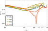 |
Fig. 17. Curvature along the separatrix in the vacuum, resistive, and FFE cases with obliquity χ = 60°. |
 |
Fig. 18. Angle between the magnetic axis and the tangent to the local magnetic field line along the separatrix in the vacuum, resistive, and FFE cases with obliquity χ = 60°. |
4.5. Multi-wavelength light curves
Radio emission is generated well inside the light cylinder; therefore, we do not expect to observe a dramatic impact of resistivity on the radio pulse profiles. However, for the X-ray and γ-ray emissions, as these are generated around the light cylinder where the magnetic field geometry is strongly impacted by resistivity, we observe a significant variation in the light curves. Fig. 19 shows an example of multi-wavelength pulse profile variation due to plasma feedback. The light curves are normalised to a maximum intensity of 1. The radio profile is not impacted by resistivity, as expected. Neither the shape nor the phase appreciably changes. However, in X-rays, the pulse profiles strongly depend on the plasma regime. The number of peaks and their relative amplitudes vary with the conductivity parameter  . Finally, in γ rays, the number of peaks is preserved, but they are shifted. Moreover, their relative amplitude varies. The most important conclusion to draw from this section is that the radio pulses are not affected by the plasma current because photons are generated deep inside the magnetosphere where the static dipole geometry remains a good approximation. The same remark applies to the γ-ray emission, except for a possible phase shift of the profile. These two extreme wavebands offer a robust way to constrain the pulsar geometry, irrespective of the assumption about the particle content of the magnetosphere. Only X-rays and, to a lesser extent, γ rays could give some hints about the conductivity value
  .
.
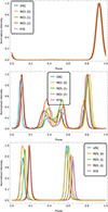 |
Fig. 19. Radio, X-ray, and γ-ray light curves, from top to bottom, for χ = 75° and ζ = 60° in the different magnetosphere models. |
As a final summary of the plethora of multi-wavelength pulse profiles that we cannot expose here, we show the radio time lag δ, i.e. the temporal delay between the first (or unique) γ-ray peak and the main radio pulse profile versus the γ-ray peak separation Δ for YPs, with periods P > 30 ms, shown with blue stars in Fig. 20. Data are taken from the 3PC catalogue (Smith et al. 2023). We also plot the expectation from our model in the different plasma regimes – from vacuum through resistive to FFE magnetospheres – in solid-coloured lines in the same Fig. 20 (see also Contopoulos & Kalapotharakos 2010 for similar results in FFE). The δ − Δ relation is rather insensitive to the plasma regime, except in an almost empty magnetosphere where the radio time lag decreases by 5% to 10%. Interestingly, this relation remains independent of the angles χ and ζ. In other words, the geometry of the pulsar need not be known. For high plasma conductivity and in FFE, we retrieve to good accuracy the relation
 (14)
(14)
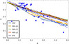 |
Fig. 20. Radio time lag δ versus γ-ray peak separation Δ. Blue stars represent data for YPs from the 3PC. The dashed black line represents the theoretical prediction (Eq. (14)), and the dashed blue line a linear fit to the data (Eq. (15)). |
as derived in Pétri (2011). This theoretical expression is shown in dashed black lines in Fig. 20. Unfortunately, this time lag is therefore not a discriminating parameter for constraining the plasma conductivity. However, in all cases, our model seems to overestimate the time lag for large peak separations satisfying Δ ≳ 0.3, although the number of observations in this range is extremely scarce. A straightforward linear fit to the observations indeed gives
 (15)
(15)
shown with the dashed blue line in Fig. 20. As shown in Pétri (2024), a purely non-radial outflow at the light cylinder can decrease the time lag to reconcile with observations. Particle-in-cell simulations and theoretical work by Contopoulos et al. (2020) indeed show that a significant velocity component exists along the azimuthal direction outside the light cylinder and is tangent to the light-cylinder surface. Such freedom would certainly better fit the data but at the expense of adding a free parameter to fix the angle between the radial direction and the velocity vector.
4.6. Beaming factor
A final interesting quantity to compare is the beaming factor fΩ, which is useful for computing the total γ-ray luminosity Lγ in the striped wind model:
 (16)
(16)
Here, D is the distance of the pulsar to the observer, and Fobs the observed flux. The factor fΩ is defined from the phase-resolved γ-ray flux Fγ(χ, ζ, φ) by Watters et al. (2009) as
 (17)
(17)
For the striped wind model, this correction factor is shown in Fig. 21 with the full dependence on obliquity χ and inclination of Earth line of sight ζE.
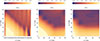 |
Fig. 21. Logarithm of the beaming factor fΩ, for the force-free magnetosphere (left), for the resistive case with |

4.7. Observational impact of the resistivity
As seen, resistivity has a strong impact on the shape of the separatrix, Fig. 6. The result is a strong variation in the X-ray pulse profile, as shown in the middle panel of Fig. 19. Moreover, in a previous work, Pétri et al. (2024) showed that this separatrix could be responsible for the non-thermal X-ray emission of pulsars. If this is confirmed in other pulsars, phase-resolved polarimetry of this non-thermal X-ray emission would strongly constrain the magnetic field geometry and height of these emission sites. Unfortunately, pulsars bright enough in X-rays are rare, and current X-ray telescopes such as Imaging X-ray Polarimetry Explorer (IXPE) are not sensitive enough to measure this polarisation.
Another approach consists of simulating pulsar populations of radio-loud and radio-quiet γ-ray pulsars and checking which resistive model better reproduces the observations, as done for instance a decade ago by Pierbattista et al. (2012, 2015, 2016). However, performing pulsar populations syntheses requires numerous input parameters for the birth, evolution, and detection of pulsars, as described in Sautron et al. (2024). Such a study would deserve a fully detailed analysis that largely goes beyond the scope of this work.
5. Conclusions
The precise plasma content of pulsar magnetospheres is still highly debated. It could exclusively contain leptonic pairs but maybe also protons and ions. Moreover the injection of these particles into the magnetosphere remains an unsolved problem. This plasma feeds back to the magnetic field structure and should lead to unambiguous observational signatures. However, we demonstrated that the radio signal is rather insensitive to the plasma resistivity. Only the X-ray and γ-ray pulse profiles are impacted by the plasma composition. The polar cap geometry remains similar in shape and size irrespective of the conductivity σ. Nevertheless, the spin-down luminosity and the magnetic field sweep-back effect in the vicinity of the light cylinder are affected, which is reflected in the γ-ray pulse profiles and their phase alignment with the radio pulse. However, we only found a weak dependence of the relation between the γ-ray peak separation Δ and the radio time lag δ.
The above approach suffers from some limitations, notably the assumption of a spatially constant and uniform conductivity σ within the magnetosphere. Regions around the neutron star could certainly be split into places where the ideal plasma regime without dissipation holds and others where dissipation occurs at a variable rate, not necessarily well described by a conductivity σ. Particle-in-cell simulations are simultaneously and self-consistently able to handle particle acceleration and radiation, but unfortunately they cannot yet handle strong magnetic field strengths of the order of 108 T. However, existing PIC simulations – even without realistic scaling – could provide hints about resistivity, informing us on the actual value of σ as a function of location within the magnetosphere. Force-free inside, dissipative outside (the so-called FIDO model; (Kalapotharakos et al. 2014)) or other approximations such as resistive magnetospheres are good alternatives to grasp the full dynamics of relativistic, strongly magnetised magnetospheres. To further discriminate between resistive magnetospheres, we need to consider the dynamics of particle acceleration to ultra-relativistic speeds, their radiation, and energetics, because curvature is strongly affected by the magnetospheric current, producing different spectra and light curves.
Acknowledgments
I am grateful to the referee for helpful comments and suggestions. This work has been supported by the grant number ANR-20-CE31-0010.
References
- Bai, X.-N., & Spitkovsky, A. 2010, ApJ, 715, 1282 [Google Scholar]
- Barnard, M., Venter, C., Harding, A. K., Kalapotharakos, C., & Johnson, T. J. 2022, ApJ, 925, 184 [NASA ADS] [CrossRef] [Google Scholar]
- Blandford, R. D. 2002, in Lighthouses of the Universe: The Most Luminous Celestial Objects and Their Use for Cosmology, eds. M. Gilfanov, R. Sunyeav, & E. Churazov (Berlin Heidelberg: Springer), ESO Astrophysics Symposia, 381 [Google Scholar]
- Bogovalov, S. V. 1999, A&A, 349, 1017 [Google Scholar]
- Brambilla, G., Kalapotharakos, C., Harding, A. K., & Kazanas, D. 2015, ApJ, 804, 84 [NASA ADS] [CrossRef] [Google Scholar]
- Cao, G., & Yang, X. 2019, ApJ, 874, 166 [Google Scholar]
- Cao, G., & Yang, X. 2020, ApJ, 889, 29 [Google Scholar]
- Cao, G., & Yang, X. 2022, ApJ, 925, 130 [Google Scholar]
- Cao, G., Zhang, L., & Sun, S. 2016a, MNRAS, 461, 1068 [NASA ADS] [CrossRef] [Google Scholar]
- Cao, G., Zhang, L., & Sun, S. 2016b, MNRAS, 455, 4267 [NASA ADS] [CrossRef] [Google Scholar]
- Cao, G., Yang, X., & Zhang, L. 2024, Universe, 10, 130 [Google Scholar]
- Cerutti, B., & Beloborodov, A. M. 2017, Space Sci Rev, 207, 111 [Google Scholar]
- Cerutti, B., Philippov, A., Parfrey, K., & Spitkovsky, A. 2015, MNRAS, 448, 606 [Google Scholar]
- Cerutti, B., Mortier, J., & Philippov, A. A. 2016a, MNRAS, 463, L89 [NASA ADS] [CrossRef] [Google Scholar]
- Cerutti, B., Philippov, A. A., & Spitkovsky, A. 2016b, MNRAS, 457, 2401 [Google Scholar]
- Chen, A. Y., & Beloborodov, A. M. 2014, ApJ, 795, L22 [NASA ADS] [CrossRef] [Google Scholar]
- Chen, A. Y., Cruz, F., & Spitkovsky, A. 2020, ApJ, 889, 69 [NASA ADS] [CrossRef] [Google Scholar]
- Contopoulos, I., & Kalapotharakos, C. 2010, MNRAS, 404, 767 [Google Scholar]
- Contopoulos, I., Pétri, J., & Stefanou, P. 2020, MNRAS, 491, 5579 [NASA ADS] [CrossRef] [Google Scholar]
- Contopoulos, I., Ntotsikas, D., & Gourgouliatos, K. N. 2024, MNRAS, 527, L127 [Google Scholar]
- Deutsch, A. J. 1955, Ann. Astrophys., 18, 1 [NASA ADS] [Google Scholar]
- Gil, J., Gronkowski, P., & Rudnicki, W. 1984, A&A, 132, 312 [NASA ADS] [Google Scholar]
- Gruzinov, A. 1999, arXiv e-prints [arXiv:astro-ph/9902288] [Google Scholar]
- Harding, A. K. 2017, Proc. Int. Astron. Union, 13, 52 [Google Scholar]
- Kalapotharakos, C., Harding, A. K., Kazanas, D., & Contopoulos, I. 2012a, ApJ, 754, L1 [Google Scholar]
- Kalapotharakos, C., Kazanas, D., Harding, A., & Contopoulos, I. 2012b, ApJ, 749, 2 [NASA ADS] [CrossRef] [Google Scholar]
- Kalapotharakos, C., Harding, A. K., & Kazanas, D. 2014, ApJ, 793, 97 [Google Scholar]
- Kalapotharakos, C., Harding, A. K., Kazanas, D., & Brambilla, G. 2017, ApJ, 842, 80 [NASA ADS] [CrossRef] [Google Scholar]
- Kalapotharakos, C., Wadiasingh, Z., Harding, A. K., & Kazanas, D. 2023, ApJ, 954, 204 [NASA ADS] [CrossRef] [Google Scholar]
- Kato, Y. E. 2017, ApJ, 850, 205 [Google Scholar]
- Kirk, J. G., Skjæraasen, O., & Gallant, Y. A. 2002, A&A, 388, L29 [NASA ADS] [CrossRef] [EDP Sciences] [Google Scholar]
- Komesaroff, M. M. 1970, Nature, 225, 612 [NASA ADS] [CrossRef] [Google Scholar]
- Li, J., Spitkovsky, A., & Tchekhovskoy, A. 2012, ApJ, 746, 60 [Google Scholar]
- Manchester, R. N., Hobbs, G. B., Teoh, A., & Hobbs, M. 2005, AJ, 129, 1993 [Google Scholar]
- Mochol, I. 2017, arXiv e-prints [arXiv:1702.00720] [Google Scholar]
- Mottez, F. 2024, A&A, 684, A115 [NASA ADS] [CrossRef] [EDP Sciences] [Google Scholar]
- Palenzuela, C. 2013, MNRAS, 431, 1853 [NASA ADS] [CrossRef] [Google Scholar]
- Pétri, J. 2011, MNRAS, 412, 1870 [Google Scholar]
- Pétri, J. 2012, MNRAS, 424, 605 [Google Scholar]
- Pétri, J. 2014, MNRAS, 439, 1071 [CrossRef] [Google Scholar]
- Pétri, J. 2015, MNRAS, 450, 714 [CrossRef] [Google Scholar]
- Pétri, J. 2016, J. Plasma Phys., 82, 635820502 [CrossRef] [Google Scholar]
- Pétri, J. 2018, MNRAS, 477, 1035 [Google Scholar]
- Pétri, J. 2019, MNRAS, 485, 4573 [CrossRef] [Google Scholar]
- Pétri, J. 2020a, Universe, 6, 15 [Google Scholar]
- Pétri, J. 2020b, MNRAS, 491, L46 [Google Scholar]
- Pétri, J. 2022, MNRAS, 512, 2854 [CrossRef] [Google Scholar]
- Pétri, J. 2024, A&A, 687, A169 [NASA ADS] [CrossRef] [EDP Sciences] [Google Scholar]
- Pétri, J., & Mitra, D. 2021, A&A, 654, A106 [NASA ADS] [CrossRef] [EDP Sciences] [Google Scholar]
- Pétri, J., Guillot, S., Guillemot, L., et al. 2024, A&A, 687, L13 [NASA ADS] [CrossRef] [EDP Sciences] [Google Scholar]
- Philippov, A., & Kramer, M. 2022, ARA&A, 60, 495 [NASA ADS] [CrossRef] [Google Scholar]
- Philippov, A. A., Spitkovsky, A., & Cerutti, B. 2015, ApJ, 801, L19 [NASA ADS] [CrossRef] [Google Scholar]
- Pierbattista, M., Grenier, I. A., Harding, A. K., & Gonthier, P. L. 2012, A&A, 545, A42 [NASA ADS] [CrossRef] [EDP Sciences] [Google Scholar]
- Pierbattista, M., Harding, A. K., Grenier, I. A., et al. 2015, A&A, 575, A3 [NASA ADS] [CrossRef] [EDP Sciences] [Google Scholar]
- Pierbattista, M., Harding, A. K., Gonthier, P. L., & Grenier, I. A. 2016, A&A, 588, A137 [NASA ADS] [CrossRef] [EDP Sciences] [Google Scholar]
- Sautron, M., Pétri, J., Mitra, D., & Dirson, L. 2024, A&A, 691, A349 [NASA ADS] [CrossRef] [EDP Sciences] [Google Scholar]
- Smith, D. A., Abdollahi, S., Ajello, M., et al. 2023, ApJ, 958, 191 [NASA ADS] [CrossRef] [Google Scholar]
- Spitkovsky, A. 2006, ApJ, 648, L51 [Google Scholar]
- Watters, K. P., Romani, R. W., Weltevrede, P., & Johnston, S. 2009, ApJ, 695, 1289 [Google Scholar]
- Yang, X., & Cao, G. 2021, ApJ, 909, 88 [Google Scholar]
- Yang, X., & Cao, G. 2024, ApJ, 964, 72 [Google Scholar]
We impose E0 > 0 and B0 = sign(E ⋅ B)|B0|.
Appendix A: Split monopole approximation
Let us assume that the magnetic axis is given by
 (A.1)
(A.1)
in a Cartesian orthonormal basis denoted by (ex, ey, ez). The current sheet is perpendicular to this vector, therefore any vector n pointing to the current sheet must satisfy μ ⋅ n = 0. Its plane is defined by
 (A.2)
(A.2)
To find the curve intersecting the light cylinder, we furthermore impose x2 + y2 = rL2 thus we write x = rL cos φ and y = rL sin φ. The vector position r of any point on the ellipse defined by the intersection of the current sheet with the light cylinder satisfies
 (A.3)
(A.3)
This vector is not normalised because ∥r∥2 = 1 + cos2φtan2 χ. If emission is radial, then the sky map is defined by a curve in the (φ, ζ) plane such that
 (A.4a)
 (A.4b)
In order to allow for a possible phase shift φ0, we use the transformation φ → φ − φ0. Fig. A.1 shows some examples of loci of this curve ζ(φ) in a sky map diagram for obliquities χ = {15° ,45° ,75° } and φ0 = 0.
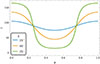 |
Fig. A.1. Loci of the γ-ray emission for the split monopole model for obliquities χ = {15° ,45° ,75° } and φ0 = 0. |
Appendix B: Current sheet dynamics
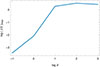 |
Fig. B.1. Maximum dissipation power in the current sheet outside the light cylinder in arbitrary units. It saturates for high conductivity, decreases for low conductivity, and vanishes for the vacuum field. |
In our simulations, the current sheet is not resolved in the force-free regime as it is theoretically of zero thickness. Even in the radiative regime, it remains at a level below the resolution of our numerical grid. However, for mildly to highly resistive solutions, the current sheet is resolved within several grid points. The maximum dissipation power computed through j ⋅ E in the current sheet outside the light cylinder is shown in Fig. B.1 for all values of the conductivity  . It obviously vanishes for the vacuum rotator and increases with increasing conductivity σ, saturating for very high conductivity
  . Radiation emanates from regions where dissipation is important. It is therefore crucial to localise where Joule heating occurs within the magnetosphere by computing the term j ⋅ E in whole space. In the force-free regime, this term vanishes identically in space by construction and in the vacuum case, it also vanishes identically because of the absence of any electric current. Only the radiative and resistive models are meaningful for studying dissipation. The region of significant dissipation outside the light cylinder, given by the extremum of the power j ⋅ E is shown in Fig. B.2 for conductivity
  from left to right. The maximum value of the power for each plot is normalised to unity for better comparison of the current sheet dissipation layer thickness. We notice that the thickness of the region of significant dissipation increases when the conductivity
  decreases, potentially impacting the width of the γ-ray pulse profiles but not their number and overall shape. However, from the location of these dissipation layers, we do not expect a significant change in the light curve phase positions.
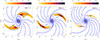 |
Fig. B.2. Isocontours of the power j ⋅ E dissipated in the current sheet outside the light cylinder for a perpendicular rotator with conductivity |
The current is known in the simulations with sufficient resistivity but its direction is not necessarily straightforwardly associated to the direction of the plasma flow or to the particle velocity, except in the fully charge-separated cases. Actually, Li et al. (2012) showed that the plasma fluid velocity is along the E ∧ B drift direction, thus no motion along the magnetic field. Fig. B.3 shows that the current is almost perfectly radial outside the light cylinder, except for significant resistivity where the current possesses a non negligible azimuthal component. So far, field lines have been used as a proxy to localise the current sheet where emission occurs but another prescription could be related to the dissipation depicted by the power j ⋅ E. This leads to a complementary way to localise the current sheet as shown in Fig. B.2. The dissipation layer location in space is consistent with the determination of the current sheet region solely by the magnetic field geometry.
 |
Fig. B.3. Cosine of the angle between the direction of the current and the radial direction for a perpendicular rotator with resistivities |
All Tables
All Figures
|
Fig. 1. Schematic view of the pulsar magnetosphere, showing the separatrix and the emission sites. |
| In the text | |
|
Fig. 2. Spin-down luminosity as a function of obliquity χ of the magnetosphere. The vacuum (VAC) and force-free (FFE) cases are shown as references. |
| In the text | |
|
Fig. 3. Spin-down luminosity for fixed obliquity χ of the magnetosphere. The vacuum (VAC) and force-free (FFE) cases are shown as limiting cases. |
| In the text | |
|
Fig. 4. Ratio Lp/L⊥vac for Γ = 10 and κ = 0 for MSPs and YPs, according to data from 3PC. |
| In the text | |
|
Fig. 5. Magnetic field lines in the equatorial plane of an orthogonal rotator for different plasma regimes going from VAC to FFE through RES. The dashed circle depicts the light-cylinder radius, and the grey disk the neutron star. |
| In the text | |
|
Fig. 6. Separatrix cross-section in the μ − Ω plane for an obliquity χ = 45° and different plasma regimes. The vertical dashed lines depict the light cylinder, while the grey disk represents the neutron star. |
| In the text | |
|
Fig. 7. Polar cap shape viewed from above for χ = {15° ,45° ,75° }, from left to right. The vacuum case is shown in dashed black lines. |
| In the text | |
|
Fig. 8. Polar cap shapes for different obliquities χ = {15° ,45° ,75° }, from left to right, and several ratios R/rL = {0.1, 0.2, 0.3}. The sizes are normalised according to the scaling with respect to |
| In the text | |
|
Fig. 9. Polar cap rim centred onto the magnetic pole for different inclination angles χ in the vacuum (left), resistive (middle), and force-free regime (right). The fit to Eq. (10) is shown as a dashed black circle of normalised radius 1.2. |
| In the text | |
|
Fig. 10. Pulse width for the radio pulse profile for χ = 60°, depending on the regime. From top to bottom: Vacuum, resistive, and force-free. The emission height along the field lines, starting from the surface, is given by s and normalised with respect to the light-cylinder radius, s/rL. |
| In the text | |
|
Fig. 11. Sky map for the radio pulse profile at χ = 60°: static dipole (dashed lines, without the 1.2 correction factor, solid lines with the 1.2 correction factor) and a force-free dipole (dotted lines). |
| In the text | |
|
Fig. 12. 3D view of the current sheet geometry for the vacuum (blue), resistive (green) and FFE (red) magnetosphere. |
| In the text | |
|
Fig. 13. γ-ray sky maps for several inclinations χ = {15° ,45° ,75° }, from top to bottom. For completeness, the radio pulse profile is also shown. The conductivity increases from left to right, starting with the vacuum case and ending with the FFE regime. The solid blue lines indicate the sky maps deduced from a static dipole for the radio profile, and the solid cyan lines indicate the sky maps deduced from the split monopole solution Eq. (13). |
| In the text | |
|
Fig. 14. Same as Fig. 13, but for the X-ray sky maps. The solid blue lines indicate the sky maps deduced from a static dipole for the radio profile, and the cyan lines for the X-ray profile. |
| In the text | |
|
Fig. 15. Curvature along the central magnetic field line for vacuum, resistive, and FFE with obliquity χ = 60°. |
| In the text | |
|
Fig. 16. Angles between the magnetic axes and the central magnetic field lines for vacuum, resistive, and FFE with obliquity χ = 60°. |
| In the text | |
|
Fig. 17. Curvature along the separatrix in the vacuum, resistive, and FFE cases with obliquity χ = 60°. |
| In the text | |
|
Fig. 18. Angle between the magnetic axis and the tangent to the local magnetic field line along the separatrix in the vacuum, resistive, and FFE cases with obliquity χ = 60°. |
| In the text | |
|
Fig. 19. Radio, X-ray, and γ-ray light curves, from top to bottom, for χ = 75° and ζ = 60° in the different magnetosphere models. |
| In the text | |
|
Fig. 20. Radio time lag δ versus γ-ray peak separation Δ. Blue stars represent data for YPs from the 3PC. The dashed black line represents the theoretical prediction (Eq. (14)), and the dashed blue line a linear fit to the data (Eq. (15)). |
| In the text | |
|
Fig. 21. Logarithm of the beaming factor fΩ, for the force-free magnetosphere (left), for the resistive case with |
| In the text | |
|
Fig. A.1. Loci of the γ-ray emission for the split monopole model for obliquities χ = {15° ,45° ,75° } and φ0 = 0. |
| In the text | |
|
Fig. B.1. Maximum dissipation power in the current sheet outside the light cylinder in arbitrary units. It saturates for high conductivity, decreases for low conductivity, and vanishes for the vacuum field. |
| In the text | |
|
Fig. B.2. Isocontours of the power j ⋅ E dissipated in the current sheet outside the light cylinder for a perpendicular rotator with conductivity |
| In the text | |
|
Fig. B.3. Cosine of the angle between the direction of the current and the radial direction for a perpendicular rotator with resistivities |
| In the text | |
Current usage metrics show cumulative count of Article Views (full-text article views including HTML views, PDF and ePub downloads, according to the available data) and Abstracts Views on Vision4Press platform.
Data correspond to usage on the plateform after 2015. The current usage metrics is available 48-96 hours after online publication and is updated daily on week days.
Initial download of the metrics may take a while.