| Issue |
A&A
Volume 706, February 2026
|
|
|---|---|---|
| Article Number | A20 | |
| Number of page(s) | 12 | |
| Section | Planets, planetary systems, and small bodies | |
| DOI | https://doi.org/10.1051/0004-6361/202557200 | |
| Published online | 30 January 2026 | |
A transiting hot Jupiter with two outer siblings orbiting an intermediate-mass post-main-sequence star
1
Max-Planck-Institut für Astronomie,
Königstuhl 17,
Heidelberg
69117,
Germany
2
European Southern Observatory,
Alonso de Córdova 3107,
Vitacura, Casilla
19001,
Santiago,
Chile
3
Facultad de Ingeniería y Ciencias, Universidad Adolfo Ibáñez,
Av. Diagonal las Torres 2640,
Peñalolén,
Santiago,
Chile
4
Millennium Institute for Astrophysics,
Chile
5
Space Telescope Science Institute,
3700 San Martin Drive,
Baltimore,
MD
21218,
USA
6
Landessternwarte, Zentrum für Astronomie der Universtät Heidelberg,
Königstuhl 12,
69117
Heidelberg,
Germany
7
Department of Astronomy, Faculty of Physics, Sofia University “St Kliment Ohridski”,
5 James Bourchier Blvd,
1164
Sofia,
Bulgaria
8
Instituto de Astrofísica, Pontificia Universidad Católica de Chile,
Av. Vicuña Mackenna 4860,
Macul,
Santiago,
Chile
9
Cerro Tololo Inter-American Observatory, CTIO/AURA Inc.,
Chile
10
Department of Physics, Engineering and Astronomy, Stephen F. Austin State University,
1936 North St,
Nacogdoches,
TX
75962,
USA
11
Department of Physics and Astronomy, The University of North Carolina at Chapel Hill,
Chapel Hill,
NC
27599-3255,
USA
12
Center for Astrophysics | Harvard & Smithsonian,
60 Garden Street,
Cambridge,
MA
02138,
USA
13
Institute of Astronomy, University of Cambridge,
Madingley Road,
Cambridge,
CB3 0HA,
UK
14
American Association of Variable Star Observers,
185 Alewife Brook Parkway, Suite 410,
Cambridge,
MA
02138,
USA
★ Corresponding author: This email address is being protected from spambots. You need JavaScript enabled to view it.
Received:
11
September
2025
Accepted:
18
November
2025
Abstract
Exoplanetary systems with multiple giant planets present an opportunity to understand planet formation, migration processes, and longterm system-wide dynamical interactions. In particular, they provide constraints to distinguish between smooth disk-driven migration or more dynamically excited system evolution pathways. We report the discovery and characterization of a unique multi-planet system hosting three gas giant planets orbiting the post-main-sequence star TOI-375. The innermost planet, TOI-375 b, was initially detected by the TESS mission, and then confirmed with photometric follow-up observations conducted using MEarth and LCOGT, and radial velocity measurements obtained with FEROS and CHIRON. The radial velocity data revealed the presence of two additional planetary candidates, TOI-375 c and TOI-375 d. We find that TOI-375 b is a hot Jupiter with an orbital period of 9.45469 ± 0.00002 days, a mass of 0.745 ± 0.053 MJ, a radius of 0.961 ± 0.043 RJ, and an eccentricity of0.087 ± 0.042. The outer two planets, TOI-375 c and TOI-375 d, are warm-cold and cold Jupiters with orbital periods of 115.5−1.6+2.0 days and 297.9−18.6+28.9 days, and minimum masses of 2.11 ± 0.22 MJ and 1.40 ± 0.28 MJ, respectively. In terms of formation and overall system architecture, the physical properties of TOI-375 b are consistent with the core accretion scenario, while the current configuration of the system could be explained by both disk-driven and high-eccentricity migration scenarios. The discovery of TOI-375 as the first known system hosting three or more fully evolved gas giants, with at least one transiting planet, makes it an excellent candidate for testing formation and migration theories.
Key words: techniques: photometric / techniques: radial velocities / planets and satellites: detection / planets and satellites: gaseous planets / planets and satellites: individual: TOI-375
© The Authors 2026
 Open Access article, published by EDP Sciences, under the terms of the Creative Commons Attribution License (https://creativecommons.org/licenses/by/4.0), which permits unrestricted use, distribution, and reproduction in any medium, provided the original work is properly cited.
This article is published in open access under the Subscribe to Open model.
Open Access funding provided by Max Planck Society.
1 Introduction
Hot Jupiters are highly irradiated gas giant exoplanets that orbit close to their host stars with orbital periods shorter than 10 days. Due to strong observational biases favoring short-period massive planets with large radii (Santerne et al. 2016), they constitute a large fraction of the well-characterized exoplanet sample despite their low occurrence rates (Stevenson 1982; Fressin et al. 2013; Mayor et al. 2011).
Standard planet formation theories struggle to explain their existence at such close-in orbits. The two dominant formation models, core accretion (Pollack et al. 1996) and gravitational instability (Cameron 1978), both predict inefficient formation in the inner disk. In these regions, high temperatures inhibit the condensation of solids and prevent either the accumulation of massive cores or disk fragmentation (Rafikov 2005; Schlichting 2014).
The relatively large number of observed hot Jupiters therefore suggests that many did not form in situ, but rather underwent orbital migration. Two primary migration mechanisms are discussed in the literature. In disk-driven migration, torques between the forming planet and the protoplanetary gas disk lead to gradual inward movement (Lin et al. 1996). Alternatively, high-eccentricity migration involves dynamical excitation of orbital eccentricity through mechanisms such as planet-planet scattering (Chatterjee et al. 2008), Kozai-Lidov cycles induced by a stellar or planetary companion (Wu & Murray 2003), or secular chaos (Wu & Lithwick 2011), followed by tidal circularization close to the star. These scenarios imply different observable outcomes in terms of orbital eccentricity, obliquity, and system architecture. Disk-driven migration typically leads to low orbital eccentricities as interactions with the protoplan-etary disk dampen eccentricities (Goldreich & Tremaine 1980; Cresswell & Nelson 2008). Planets that migrate through the disk tend to maintain low spin-orbit obliquities because the migration occurs within an aligned disk (Lin et al. 1996; Dawson & Johnson 2018), and the mutual inclinations between planets are expected to remain small (Kley & Nelson 2012). These systems often host multiple co-planar companions (Libert & Tsiganis 2011), and show a smooth distribution of orbital periods as planets migrate inward (Mordasini et al. 2009). The transit probability of outer planets remains high due to their low mutual inclinations (Dawson & Chiang 2014), and minimal tidal heating or eccentricity evolution is expected over time (Kley & Nelson 2012).
In contrast, high-eccentricity migration involves dynamical perturbations such as planet-planet scattering or Kozai-Lidov cycles that excite eccentric and inclined orbits before tidal forces circularize them (Chatterjee et al. 2008; Naoz 2016). This process often produces high stellar obliquities, including retrograde orbits (Albrecht et al. 2012). Systems that undergo this pathway frequently contain isolated hot Jupiters or have distant inclined companions (Winn et al. 2010; Bryan et al. 2016). Their orbital period distribution shows a pile-up of hot Jupiters at short periods due to tidal circularization (Santerne et al. 2016). The outer planets in such systems have a low transit probability because of their mutually inclined orbits (Read et al. 2017), and the presence of tidal signatures or an eccentricity-age correlation may indicate ongoing orbital evolution (Lai 2012).
Well-characterized multi-planet systems provide key constraints to test these formation and migration pathways. The presence, proximity, and physical properties of planetary companions can help distinguish between smooth disk-driven migration and more violent dynamically excited evolution. This means that characterizing the architectures of systems hosting hot and cold Jupiters is crucial to understanding giant planet origins and orbital evolution.
The Transiting Exoplanet Survey Satellite (TESS; Ricker et al. 2015) is a space-based mission designed to search for exoplanets around bright nearby stars by monitoring their light for periodic dips caused by planetary transits. By surveying nearly the entire sky, TESS has enabled the identification of thousands of planetary candidates, many of which orbit stars suitable for follow-up observations. Its high-precision photometry and wide coverage make it particularly effective at detecting short-period planets and systems with multiple transiting planets, providing a valuable starting point for characterizing planetary architectures and informing studies of formation and migration. In this work, we take a close look at TOI-375, an intermediate-mass (M* ≳ 1.3 M⊙) evolved star that hosts a hot Jupiter detected by the TESS mission and two outer gaseous companions, subsequently detected by radial velocity follow-up.
The paper is structured as follows. In Sect. 2, we describe the observational material used to perform a global modeling of the system, as described in Sect. 3. The results are then discussed in Sect. 4 and our conclusions are presented in Sect. 5.
Observation details for TESS sectors that contain observations of TOI-375.
2 Observations
2.1 TESS
TOI-375 was observed by the Transiting Exoplanet Survey Satellite over multiple sectors during its operational period. Initial observations were conducted at 30-minute cadence during Sectors 1 and 2, followed by 2-minute cadence observations in Sectors 13, 27, 28, 39, 66, 67, and 68. The TESS data-validation reports revealed a transiting exoplanet candidate with a 9.45-day period and an approximate transit depth of 1000 ppm. The complete TESS observation log is presented in Table 1.
2.2 Ground-based photometry
In addition to TESS observations, ground-based photometric monitoring of TOI-375 was conducted using Las Cumbres Observatory Global Telescope (LCOGT; Brown et al. 2013) 1.0 m network from 12.10.2019 to 26.10.2019, and MEarth-South from 12.08.2019 to 21.08.2019. The LCOGT 1 m telescopes are equipped with 4096 × 4096 SINISTRO cameras having an image scale of 0″.389 per pixel, resulting in a 26′ × 26′ field of view. The LCOGT images were calibrated by the standard LCOGT BANZAI pipeline (McCully et al. 2018) and differential photometric data were extracted using AstroImageJ (Collins et al. 2017). While three transit ingresses and a single egress were observed according to the ephemeris from the last TESS data-validation report, the shallow transit depth requires optimal observing conditions to extract meaningful information. Consequently, our analysis incorporates only two partial transit observations: an ingress detected by LCOGT at the South African Astronomical Observatory (SAAO) on 09 September 2019, and another ingress observed by MEarth-South on 21 August 2019. The complete ground-based observation log is presented in Table 2.
2.3 Spectroscopy
We obtained 66 high-resolution spectra of TOI-375 between 2018 and 2019 using the Fiber-fed Extended Range Optical Spectrograph (FEROS) and CHIRON spectrographs located in Chile.
Ground-based observations.
2.3.1 FEROS
The majority of our spectroscopic dataset consists of observations conducted with the FEROS spectrograph (Kaufer et al. 1999), mounted on the MPG 2.2 m telescope at La Silla Observatory. Between 07 February 2019 and 17 November 2019, we obtained 49 observations using simultaneous calibration mode, where a thorium-argon (ThAr) lamp was observed through the secondary fiber to track instrumental drifts caused by environmental variations during science exposures.
The data were reduced using the CERES pipeline (Brahm et al. 2017a), which delivers radial velocities corrected for both instrumental drift and Earth’s motion. These velocities were derived using the cross-correlation technique, employing a G2-type binary mask as the template spectrum. The pipeline additionally computes bisector span measurements from the cross-correlation peak and provides preliminary stellar parameters through comparison of the continuum-normalized spectrum with a grid of synthetic spectra. The latest version of CERES also includes stellar activity indicators.
2.3.2 CHIRON
We also collected 16 spectra using the CHIRON high-resolution spectrograph (Tokovinin et al. 2013) between 21 October 2018 and 15 October 2019. CHIRON is mounted on the SMARTS 1.5 m telescope at the Cerro Tololo Inter-American Observatory and is fed by an octagonal multi-mode optical fiber. We utilized the image slicer mode, which provides high throughput at a spectral resolution of R ≈ 80 000. Our exposure times ranged from 750 to 1200 s, yielding a signal-to-noise ratio (S/N) per extracted pixel in the range ≈20-35.
The radial velocities were computed via cross-correlation between individual spectra and a high-resolution stellar template created by co-adding all observations of the target. In contrast to FEROS, CHIRON lacks a simultaneous calibration capability. Therefore, we obtained Th-Ar lamp spectra before the science observations to correct for instrumental drift. This methodology achieves long-term RV stability of <10 ms 1 for bright targets (texp < 60s) and <15ms−1 for fainter objects (texp < 1800 s). For the detailed methodology we refer to Wang et al. (2019) and Jones et al. (2019). A subset of observations obtained during August-September 2019 was acquired at a lower spectral resolution, and therefore required independent reduction procedures.
Stellar properties of TOI-375.
3 Analysis
3.1 Stellar parameters
We used Species (Soto & Jenkins 2018) to derive the stellar atmospheric and bulk parameters, using a high signal-to-noise ratio template, produced by co-adding the individual FEROS data. This code has been adapted to robustly derive the stellar parameters of evolved stars (Soto et al. 2021). Briefly, Species measures the equivalent widths of the iron line and solves the radiative transfer equation under the assumption of local thermodynamic equilibrium to obtain the effective temperature (Teff), surface gravity (log g), metallicity ([Fe/H]), and microturbulent velocity (ξt). From these values, Species estimates the chemical abundances, projected rotation velocity (v sin i), and macroturbulent velocity, and, through Bayesian interpolation on a grid of MIST isochrones (Dotter 2016), the stellar mass, radius, and age. For this work we modified the code to incorporate parallaxes, proper motions, and magnitudes from Gaia DR3, and we increased the range of default priors to allow for higher extinction values (AV). This was needed given the large interstellar absorption in the line of sight. The derived stellar properties indicate a G8 IV spectral type and are listed in Table 3.
Figure 1 shows the position of TOI-375 in the HR diagram, along with different PARSEC evolutionary models. The 1.45 M⊙ model with Z = 0.020 (corresponding to [Fe/H] = +0.11 dex) is the closest one to its position in the grid. As can be seen, this star is currently at the end of the subgiant branch phase, hence manifesting a rapidly shrinking H-burning shell around the (nearly) iso-thermal He-rich core, and is about to start climbing the red giant branch.
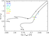 |
Fig. 1 Position of TOI-375 in the HR diagram (black star), using the stellar parameters derived here (see Table 3). For comparison, the position of known giant stars hosting transiting giant planets are overplotted. Two different PARSEC models (Bressan et al. 2012) for 1.0 and 1.45 M⊙, are overplotted. The solid and dotted lines correspond to Z* =0.017 and 0.020, respectively. |
3.2 Nearby companions
Since the planetary radius is determined from the relative stellar flux decrease during transit, accounting for contamination from nearby stars is crucial. Without this correction, the planetary radius can be underestimated due to overestimating the host star’s contribution to the out-of-transit baseline flux. This contamination effect, known as dilution, can be accounted for by incorporating a dilution factor in the light curve model, which represents the fraction of the out-of-transit flux originating from the host star. To assess possible contamination, we examined target pixel file (TPF) images with tpfplotter (Aller et al. 2020), utilizing stellar positions and magnitudes from the Gaia catalog (Fig. A.1). We also searched for closer stellar companions to TOI-375 using speckle imaging with the 4.1 m Southern Astrophysical Research (SOAR) telescope (Tokovinin 2018). The target was observed with HRCam on 2019 February 2. This observation was sensitive to companions up to 4.9 magnitudes at 1 arcsec (Ziegler et al. 2020, 2021). The 5σ detection limits and the speckle autocorrelation function from this observation are shown in Fig. 2. No nearby sources were detected within 3 arcsec of TOI-375.
Both analyses show no evidence of contamination within the photometric aperture in any TESS sector, allowing us to adopt a dilution factor of unity in subsequent analyses.
3.3 Light curve analysis
We analyzed photometric data from both space-based TESS observations and ground-based facilities. For TESS Sectors 1 and 2, we extracted light curves from the full frame images using tesseract, while for Sectors 13 through 68 we utilized the Pre-search Data Conditioning Simple Aperture Photometry (PDC-SAP) flux retrieved from the MAST portal. The photometric data from LCOGT was automatically reduced using the BANZAI pipeline (McCully et al. 2018), which outputs the light curve for different aperture sizes. Since no contamination from nearby sources was present, we selected the largest available aperture of 6 arcsecond. The MEarth-South observations were processed following the reduction techniques described in Irwin et al. (2007) and Irwin & Lewis (2001). The dataset includes simultaneous aperture photometry from telescopes 11 through 17, which we combined into a single light curve for our analysis.
To search for periodic transit signals, we first detrended the TESS light curves using a linear model and performed a Transit Least Squares (TLS) analysis (Hippke & Heller 2019) using exostriker (Trifonov 2019). This analysis revealed a strong signal with a signal detection efficiency (SDE) of approximately 73, corresponding to the 9.45-day period planet previously reported in the TESS data validation reports. While additional peaks were detected in the periodogram, we identified them as harmonics of the primary signal.
After obtaining a preliminary transit model for the 9.45-day planet candidate, we conducted a subsequent TLS analysis on the residuals using exostriker to search for additional periodic signals. This analysis revealed no additional signals that could indicate the presence of other transiting planets. However, we identified a potential single transit event in Sector 2 at around BJD 2458365.82 (Fig. 4). This region of the light curve exhibits particularly high noise levels, and requires further observations to confirm whether this signal corresponds to a planetary transit. Therefore, we did not include it in our final analysis.
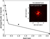 |
Fig. 2 Speckle autocorrelation function for TOI-375, obtained with the SOAR telescope. The black dots represent the 5σ contrast curve, and the solid line shows a linear fit to the data at separations smaller and larger than ~0.2 arcsec. |
3.4 Radial-velocity analysis
The generalized Lomb-Scargle (GLS) periodograms (Zechmeister & Kürster 2009) of the FEROS radial velocity data reveal strong periodic signals at 289, 118, and 47 days, all well below the 0.1% false-alarm probability (FAP; Fig. 3). An additional weak signal is detected at 9.43 days, corresponding to the transiting planet identified by TESS. In contrast, standard stellar activity indicators, including the bisector (BIS; Queloz et al. 2001; Santos et al. 2014), Hα (Robertson et al. 2013), and chromospheric indices such as the S-index (Noyes et al. 1984), show no significant power at these periods, suggesting that the radial velocity variations are unlikely to be driven by stellar activity. The full width at half maximum (FWHM) exhibits peaks between the 1-0.1% FAP range at around 104 and 342 days, but these signals are much weaker than those observed in the radial velocities at similar periods. The window function (WF) shows a peak at 83 days, which does not coincide with any of the radial velocity signals, indicating that the observed RV variations are unlikely to arise from the temporal sampling of the data.
To fit the radial velocities, we used the juliet library (Espinoza et al. 2019). To select the best-fitting model, we employed a Bayesian model comparison approach. We computed the Akaike information criterion (AIC) and the Bayesian information criterion (BIC) for 16 different models that combine circular and eccentric orbits for planet c (with orbital periods between 50 and 150 days) and planet d (between 200 and 450 days). We also tested for the presence of a linear trend in the data. The best-fitting model includes no linear trend and adopts circular orbits for the outer planets, suggesting that the available data are insufficient to constrain their eccentricities. Additionally, we tested the presence of a planet corresponding to the 47-day signal, but this peak in the GLS periodogram corresponds to a harmonic of the 9.45-day planet and does not indicate a real planetary signal.
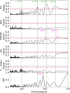 |
Fig. 3 Periodogram of the radial velocities (top) and activity indices (middle), along with the window function of the observations (bottom) for the FEROS data of TOI-375. False-alarm probabilities are indicated by horizontal lines: dashed red for 1% FAP and dotted blue for 0.1% FAP in each panel. The green vertical lines mark peaks in the radial-velocity periodogram with a FAP below 1% or corresponding to a confirmed a priori planetary signal, such as the 9.4-day signal. In contrast, the magenta vertical lines indicate signals that are unlikely to be of planetary origin. |
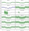 |
Fig. 4 Phase-folded light curves (in green) from each instrument (or sector in the case of TESS) with the best-fit transit model for TOI-375 b derived using juliet. Also shown is the potential single transit event (in blue) of one of the outer planets on TESS sector 2. Data points are shown in their original time sampling (small green or blue points) and binned in phase with 6 minute intervals (white markers). The solid black line represents the best-fit transit model. We do not include the transit of TOI-375 c in the final model as there is not enough evidence to support that it has a true planetary origin. |
3.5 Global modeling
We used (Espinoza et al. 2019) to jointly model the radial velocities and light curves of TOI-375. We adopted non-informative priors for all parameters except for the stellar density, for which we used a normal prior centered on the value derived with Species, with a standard deviation corresponding to its reported uncertainty. The full list of priors is presented in Table A.2. In order to remove systematic effects from the light curves, we implemented different de-trending techniques for each instrument simultaneously during the global modeling of the system. For TESS Sectors 1 and 2, we implemented Gaussian processes using a Celerite Matérn kernel (Foreman-Mackey 2018) to account for correlated noise in the data. For the remaining TESS sectors (13-68), we utilized the PDC-SAP flux. These light curves have already undergone systematic correction through the PDC pipeline and we only normalized it by the median of the baseline flux. The LCOGT observations from SAAO were detrended using a two-dimensional linear model with time and airmass as regressors, accounting for both temporal trends and atmospheric effects. For MEarth data, we implemented a two-dimensional linear model using time and FWHM as regressors, supplemented by Gaussian processes with a Matérn kernel using time as the regressor to capture additional correlated noise patterns.
To select the limb darkening law, we adopted the logarithmic limb darkening law based on the recommendations listed in Espinoza & Jordán (2016), who studied the performance of different laws across a range of stellar and planetary parameters. For stars with effective temperatures around 5100 K, planet-to-star radius ratios near 0.035, and impact parameters between 0.35 and 0.55, the logarithmic law was found to perform optimally. Since limb darkening is wavelength dependent and can show different values depending on the photometric band used for the observations, we provide independent priors for LCOGT, MEarth, and TESS, but group all TESS sectors together as they should exhibit consistent limb darkening behavior.
The posteriors of the physical parameters and ephemeris for the TOI-375 b, c, and d are presented in Table 4. The best-fit lines for the transit and radial velocity parts of the model are shown in Figs. 4 and 5, respectively.
3.6 Transit timing variations
Transit timing variations (TTVs) are a powerful tool for detecting additional planets in a system and measuring planetary masses through gravitational interactions. For systems with multiple planets such as TOI-375, TTV detection in the inner transiting planet could provide independent mass measurements of the outer companions (Agol & Fabrycky 2018).
To search for transit timing variations, we used Juliet to model the light curve, including the TESS sectors utilized for the joint analysis of the system, and the sectors 89, 93, 94, 95, and 96, which were released during the course of this study. For the prior distributions, we used the posteriors of the joint model. We included the transit perturbations for each transit with a Gaussian prior with σ = 0.1 days to allow for potential timing deviations from the linear ephemeris in the joint model. In Fig. 6 we show the TTVs over the span of the observations, as well as the Lomb-Scargle periodogram. No significant TTV signal is detected for TOI-375 b.
4 Discussion
4.1 System dynamical history
Systems hosting three or more Jupiter-mass planets are uncommon, and cases where at least one of them transits are even rarer. To date, only one other such system, V1298 Tau (David et al. 2019; Feinstein et al. 2022), has been reported (Fig. 7). We note, however, that V1298 Tau is very young (~20-30 Myr), and the gas giants in this system are more likely super-Earths or mini-Neptunes still in the process of contraction, mass loss, or both (Thao et al. 2024; Barat et al. 2025). This makes TOI-375 especially valuable for testing theories of system evolution and migration.
The low eccentricity of TOI-375b is consistent with disk-driven migration, where the planet forms beyond the snow line and migrates inward through the protoplanetary disk while maintaining low eccentricity and inclination (Lin et al. 1996; Kley & Nelson 2012). If the outer planets also have low eccentricities, which is a reasonable assumption given the current data, the system architecture would further support this formation pathway. High-eccentricity migration mechanisms, such as planet-planet scattering or Kozai-Lidov cycles, are expected to produce systems with higher eccentricities, misaligned orbits, and fewer nearby companions (Chatterjee et al. 2008; Naoz 2016).
The lack of evidence of strong radial velocity trends or orbital instability suggests that the system is dynamically stable. However, without precise measurements of eccentricity and mutual inclinations, it is not possible to rule out past dynamical interactions such as mild scattering or secular perturbations.
Overall, the data are consistent with a formation scenario involving disk-driven migration for TOI-375b, accompanied by two outer giant planets on wider orbits. Additional observations, especially those that can constrain orbital inclinations and spin-orbit alignment, would help clarify the system’s dynamical history.
Physical parameters and ephemeris for TOI-375 b, c, and d. BJD* = BJD - 2458000.
4.2 TOI-375 b interior modeling
We computed interior models of TOI-375 b using the Modules for Experiments in Stellar Astrophysics (MESA; Paxton et al. 2011), closely following the methodology described in Jones et al. (2024) and Tala Pinto et al. (2025). The interior of the planet is modeled with a rocky-core surrounded by a gas rich H-He envelope. For this, we assumed an inert homogeneous core composed of a 1:1 mixture of rock and ice, whose density is computed using the Hubbard & Marley (1989) ρ - P tables (in this case ρc = 9 g cm−3). The metallicity of the envelope is assumed to be the same as the host star (Zenv = 0.015). Finally, the instant irradiation level received by the planet is also updated in steps of 250 Myr, using the PARSEC model that better matches the host star parameters. Figure 10 shows the resulting changes in the equilibrium temperature of the planet over time. Figure 9 shows the position of TOI-375 b in the age-radius diagram. Different models with core masses between 28-49 M⊙ that reproduce its position within 1 σ are overplotted. This corresponds to a planet metallicity of Z = 0.18 , hence a planet heavy-elementenrichment of Zp/Z* = 10.0
 , in agreement with the coreaccretion model of planet formation (Fig. 8). In addition, despite the high irradiation level of fp ~ 8 × 10⁸ (erg s−1 cm−2 ) currently received by the planet, no evidence of (re-)inflation is observed (Demory & Seager 2011; Grunblatt et al. 2016).
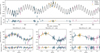 |
Fig. 5 Top : radial velocities along with the median model (black line) for TOI-375. Our model is composed of three different Keplerian components. Bottom : Keplerian components of the full model presented in the top panel. The 9.4-day variation is from TOI-375 b, the transiting exoplanet detected by TESS. The two additional 118.7 and 289.9-day signals observed in our radial-velocities have been identified as likely candidate exoplanets (c and d) given no obvious stellar activity origin. |
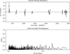 |
Fig. 6 Top : transit timing residuals (∆T) as a function of time for TOI-375 b. ∆T represents the observed transit times minus the calculated times from the linear ephemeris of the joint model. Bottom : Lomb-Scargle periodogram of the TTV signal. |
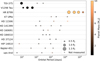 |
Fig. 7 Systems with three or more planets in the mass range 0.3 MJ < M < 30 MJ. Planets shown with a cross lack radius measurements, and the mass used corresponds to the minimum mass (Msin(i)). TOI-375 represents the second ever discovery of a multi-Jupiter-mass system where at least one planet’s transit has been detected. |
4.3 Prospects for atmospheric characterization
We assessed the feasibility of performing transmission spectroscopy of the inner planet by calculating the transmission spectroscopy metric (TSM) following Kempton et al. (2018). For planets of comparable size, a TSM above 90 is recommended; we obtained a TSM of ~12, which indicates TOI-375 b has very limited potential for transmission spectroscopy. Consequently, future observations of this system should focus on the detection of the two outer planets and understanding the dynamical history of the system.
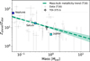 |
Fig. 8 Metal enrichment as a function of mass for gas giants. The mass-metallicity trend and sample data are provided by (T16 Thorngren et al. 2016). |
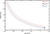 |
Fig. 9 Position of TOI-375 b in the age-radius diagram (black dot) and planet evolutionary models with core masses of 28, 49, and 49 M⊕. |
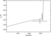 |
Fig. 10 Equilibrium temperature as a function of the system age (solid line), computed using the closest model in the PARSEC grid (M* = 1.45 M⊙; Z* = 0.20; see Fig. 1). The position of TOI-375 b is overplotted (black dot). |
5 Summary
In this work, we analyzed the radial velocity and transit photometry data of the post-main-sequence star TOI-375. Our best-fit model includes three Keplerian components corresponding to a hot, a warm, and a cold Jupiter.
TOI-375 b is a hot Jupiter (Teq ≈ 1373 K) in a close-in orbit (a ≈ 0.1 au, P ≈ 9.45 days) with low orbital eccentricity (e ≈ 0.09), and a well-constrained radius and mass from photometry and radial velocity measurements (Rp ≈ 0.96 and Mp ≈ 0.74). The two additional companions, TOI-375 c and TOI-375 d, orbit at larger separations (a ≈ 0.52 and 0.98 au) with minimum masses of approximately 2.04 and 1.35 MJ, respectively. No transits have been detected with a high degree of confidence for these outer planets, and their radii and orbital inclinations are unconstrained.
The system architecture is consistent with a formation scenario involving disk-driven migration. Additional data are required to rule out high-eccentricity migration pathways. Furthermore, our interior modeling of TOI-375 b supports formation via core accretion, in line with current planet formation theory.
TOI-375 is the first confirmed system with three or more fully evolved Jupiter-mass planets, where at least one of the planets is transiting, making it a valuable case study for future work.
Data availability
The data underlying this article and Tables rvs.csv and lc.csv are available at the CDS via https://cdsarc.cds.unistra.fr/viz-bin/cat/J/A+A/706/A20.
Acknowledgements
Y.R. would like to thank the Millennium Institute of Astrophysics (MAS) and FONDECYT for supporting this research. N.E. would like to thank the Gruber Foundation for its generous support to this research. R.B. acknowledges support from FONDECYT Project 1241963 and from ANID -Millennium Science Initiative - ICN12_009. A.J. acknowledges support from FONDECYT project 1171208 and by the Ministry for the Economy, Development, and Tourism’s Programa Iniciativa Científica Milenio through grant IC 120009, awarded to the Millennium Institute of Astrophysics (MAS). M.B. acknowledges CONICYT-GEMINI grant 32180014. T.D. acknowledges support from MIT’s Kavli Institute as a Kavli postdoctoral fellow. Resources supporting this work were provided by the NASA High-End Computing (HEC) Program through the NASA Advanced Supercomputing (NAS) Division at Ames Research Center for the production of the SPOC data products. This work makes use of observations from the LCOGT network. Part of the LCOGT telescope time was granted by NOIRLab through the Mid-Scale Innovations Program (MSIP). MSIP is funded by NSF. This research has made use of the Exoplanet Follow-up Observation Program (ExoFOP; DOI: 10.26134/Exo-FOP5) website, which is operated by the California Institute of Technology, under contract with the National Aeronautics and Space Administration under the Exoplanet Exploration Program. Funding for the TESS mission is provided by NASA’s Science Mission Directorate. K.A.C. acknowledges support from the TESS mission via subaward s3449 from MIT. This work has made use of data from the European Space Agency (ESA) mission Gaia (https://www.cosmos.esa.int/gaia), processed by the Gaia Data Processing and Analysis Consortium (DPAC, https://www.cosmos.esa.int/web/gaia/dpac/consortium). Funding for the DPAC has been provided by national ins titutions, in particular the institutions participating in the Gaia Multilateral Agreement. This research made use of exoplanet (Foreman-Mackey et al. 2019) and its dependencies (Astropy Collaboration 2013, 2018; Espinoza 2018; Foreman-Mackey et al. 2019; Kipping 2013; Luger et al. 2019; Salvatier et al. 2016; Theano Development Team 2016). We acknowledge the use of the following facilities: TESS, FEROS/MPG 2.2m, NRES/LCOGT 1m, CTIO 1.5m/CHIRON, SINISTRO/LCOGT 1 m, and MEarth-South. We also acknowledge the use of the following software: CERES (Brahm et al. 2017a; Jordán et al. 2014), ZASPE (Brahm et al. 2017b, 2015), SPECIES (Soto & Jenkins 2018), radvel (Fulton et al. 2018), batman (Kreidberg 2015), MultiNest (Feroz et al. 2009), exoplanet (Foreman-Mackey et al. 2019), juliet (Espinoza et al. 2019), AstroImageJ (Collins et al. 2017), TAPIR (Jensen 2013), and exostriker (Trifonov 2019).
References
- Agol, E., & Fabrycky, D. C. 2018, in Handbook of Exoplanets, eds. H. J. Deeg, & J. A. Belmonte, 7 [Google Scholar]
- Albrecht, S., Winn, J. N., Fabrycky, D. C., Torres, G., & Setiawan, J. 2012, in IAU Symposium, 282, From Interacting Binaries to Exoplanets: Essential Modeling Tools, eds. M. T. Richards, & I. Hubeny, 397 [Google Scholar]
- Aller, A., Lillo-Box, J., Jones, D., Miranda, L. F., & Barceló Forteza, S. 2020, A&A, 635, A128 [NASA ADS] [CrossRef] [EDP Sciences] [Google Scholar]
- Astropy Collaboration (Robitaille, T. P., et al.) 2013, A&A, 558, A33 [NASA ADS] [CrossRef] [EDP Sciences] [Google Scholar]
- Astropy Collaboration (Price-Whelan, A. M., et al.) 2018, AJ, 156, 123 [Google Scholar]
- Barat, S., Désert, J.-M., Mukherjee, S., et al. 2025, AJ, 170, 165 [Google Scholar]
- Brahm, R., Jordán, A., Hartman, J. D., et al. 2015, AJ, 150, 33 [Google Scholar]
- Brahm, R., Jordán, A., & Espinoza, N. 2017a, PASP, 129, 034002 [Google Scholar]
- Brahm, R., Jordán, A., Hartman, J., & Bakos, G. 2017b, MNRAS, 467, 971 [NASA ADS] [Google Scholar]
- Bressan, A., Marigo, P., Girardi, L., et al. 2012, MNRAS, 427, 127 [NASA ADS] [CrossRef] [Google Scholar]
- Brown, T. M., Baliber, N., Bianco, F. B., et al. 2013, PASP, 125, 1031 [Google Scholar]
- Bryan, M. L., Knutson, H. A., Howard, A. W., et al. 2016, ApJ, 821, 89 [NASA ADS] [CrossRef] [Google Scholar]
- Cameron, A. G. W. 1978, Moon Planets, 18, 5 [Google Scholar]
- Chatterjee, S., Ford, E. B., Matsumura, S., & Rasio, F. A. 2008, ApJ, 686, 580 [NASA ADS] [CrossRef] [Google Scholar]
- Collins, K. A., Kielkopf, J. F., Stassun, K. G., & Hessman, F. V. 2017, AJ, 153, 77 [Google Scholar]
- Cresswell, P., & Nelson, R. P. 2008, A&A, 482, 677 [NASA ADS] [CrossRef] [EDP Sciences] [Google Scholar]
- David, T. J., Cody, A. M., Hedges, C. L., et al. 2019, AJ, 158, 79 [NASA ADS] [CrossRef] [Google Scholar]
- Dawson, R. I., & Chiang, E. 2014, Science, 346, 212 [Google Scholar]
- Dawson, R. I., & Johnson, J. A. 2018, Annu. Rev. A&A, 56, 175 [Google Scholar]
- Demory, B.-O., & Seager, S. 2011, ApJS, 197, 12 [NASA ADS] [CrossRef] [Google Scholar]
- Dotter, A. 2016, ApJS, 222, 8 [Google Scholar]
- Espinoza, N. 2018, RNAAS, 2, 209 [Google Scholar]
- Espinoza, N., & Jordán, A. 2016, MNRAS, 457, 3573 [NASA ADS] [CrossRef] [Google Scholar]
- Espinoza, N., Kossakowski, D., & Brahm, R. 2019, MNRAS, 490, 2262 [Google Scholar]
- Feinstein, A. D., David, T. J., Montet, B. T., et al. 2022, ApJ, 925, L2 [NASA ADS] [CrossRef] [Google Scholar]
- Feroz, F., Hobson, M. P., & Bridges, M. 2009, MNRAS, 398, 1601 [NASA ADS] [CrossRef] [Google Scholar]
- Foreman-Mackey, D. 2018, RNAAS, 2, 31 [NASA ADS] [Google Scholar]
- Foreman-Mackey, D., Czekala, I., Agol, E., et al. 2019, https://doi.org/10.5281/zenodo.3359880 [Google Scholar]
- Fressin, F., Torres, G., Charbonneau, D., et al. 2013, ApJ, 766, 81 [NASA ADS] [CrossRef] [Google Scholar]
- Fulton, B. J., Petigura, E. A., Blunt, S., & Sinukoff, E. 2018, arXiv e-prints [arXiv:1801.01947] [Google Scholar]
- Goldreich, P., & Tremaine, S. 1980, ApJ, 241, 425 [Google Scholar]
- Grunblatt, S. K., Huber, D., Gaidos, E. J., et al. 2016, AJ, 152, 185 [NASA ADS] [CrossRef] [Google Scholar]
- Hippke, M., & Heller, R. 2019, A&A, 623, A39 [NASA ADS] [CrossRef] [EDP Sciences] [Google Scholar]
- Hubbard, W., & Marley, M. S. 1989, Icarus, 78, 102 [NASA ADS] [CrossRef] [Google Scholar]
- Irwin, M., & Lewis, J. 2001, New Astr. Rev., 45, 105 [Google Scholar]
- Irwin, J., Irwin, M., Aigrain, S., et al. 2007, MNRAS, 375, 1449 [Google Scholar]
- Jensen, E. 2013, Tapir: A web interface for transit/eclipse observability, Astrophysics Source Code Library [record ascl:1306.007] [Google Scholar]
- Jones, M. I., Brahm, R., Espinoza, N., et al. 2019, A&A, 625, A16 [NASA ADS] [CrossRef] [EDP Sciences] [Google Scholar]
- Jones, M. I., Reinarz, Y., Brahm, R., et al. 2024, A&A, 683, A192 [NASA ADS] [CrossRef] [EDP Sciences] [Google Scholar]
- Jordán, A., Brahm, R., Bakos, G. Á., et al. 2014, AJ, 148, 29 [CrossRef] [Google Scholar]
- Kaufer, A., Stahl, O., Tubbesing, S., et al. 1999, The Messenger, 95, 8 [Google Scholar]
- Kempton, E. M.-R., Bean, J. L., Louie, D. R., et al. 2018, PASP, 130, 114401 [CrossRef] [Google Scholar]
- Kipping, D. M. 2013, MNRAS, 435, 2152 [Google Scholar]
- Kley, W., & Nelson, R. P. 2012, ARA&A, 50, 211 [Google Scholar]
- Kreidberg, L. 2015, PASP, 127, 1161 [Google Scholar]
- Lai, D. 2012, MNRAS, 423, 486 [NASA ADS] [CrossRef] [Google Scholar]
- Libert, A.-S., & Tsiganis, K. 2011, MNRAS, 412, 2353 [Google Scholar]
- Lin, D. N. C., Bodenheimer, P., & Richardson, D. C. 1996, Nature, 380, 606 [Google Scholar]
- Luger, R., Agol, E., Foreman-Mackey, D., et al. 2019, AJ, 157, 64 [Google Scholar]
- Mayor, M., Marmier, M., Lovis, C., et al. 2011, arXiv e-prints [arXiv:1109.2497] [Google Scholar]
- McCully, C., Turner, M., Volgenau, N., et al. 2018, https://doi.org/10.5281/zenodo.1257560 [Google Scholar]
- McCully, C., Volgenau, N. H., Harbeck, D.-R., et al. 2018, SPIE Conf. Ser., 10707, 107070K [Google Scholar]
- Mordasini, C., Alibert, Y., Benz, W., & Naef, D. 2009, A&A, 501, 1161 [NASA ADS] [CrossRef] [EDP Sciences] [Google Scholar]
- Naoz, S. 2016, Annu. Rev. A&A, 54, 441 [Google Scholar]
- Noyes, R. W., Hartmann, L. W., Baliunas, S. L., Duncan, D. K., & Vaughan, A. H. 1984, ApJ, 279, 763 [Google Scholar]
- Paxton, B., Bildsten, L., Dotter, A., et al. 2011, ApJS, 192, 3 [Google Scholar]
- Pollack, J. B., Hubickyj, O., Bodenheimer, P., et al. 1996, Icarus, 124, 62 [NASA ADS] [CrossRef] [Google Scholar]
- Queloz, D., Henry, G. W., Sivan, J. P., et al. 2001, A&A, 379, 279 [NASA ADS] [CrossRef] [EDP Sciences] [Google Scholar]
- Rafikov, R. R. 2005, ApJ, 621, L69 [Google Scholar]
- Read, M. J., Wyatt, M. C., & Triaud, A. H. M. J. 2017, MNRAS, 469, 171 [NASA ADS] [CrossRef] [Google Scholar]
- Ricker, G. R., Winn, J. N., Vanderspek, R., et al. 2015, J. Astron. Telesc. Instrum. Syst., 1, 014003 [Google Scholar]
- Robertson, P., Endl, M., Cochran, W. D., & Dodson-Robinson, S. E. 2013, ApJ, 764, 3 [Google Scholar]
- Salvatier, J., Wiecki, T. V., & Fonnesbeck, C. 2016, PeerJ Comput. Sci., 2, e55 [Google Scholar]
- Santerne, A., Moutou, C., Tsantaki, M., et al. 2016, A&A, 587, A64 [NASA ADS] [CrossRef] [EDP Sciences] [Google Scholar]
- Santos, N., Mortier, A., Faria, J., et al. 2014, A&A, 566 [Google Scholar]
- Schlichting, H. E. 2014, ApJ, 795, L15 [Google Scholar]
- Soto, M. G., & Jenkins, J. S. 2018, A&A, 615, A76 [NASA ADS] [CrossRef] [EDP Sciences] [Google Scholar]
- Soto, M. G., Jones, M. I., & Jenkins, J. S. 2021, A&A, 647, A157 [NASA ADS] [CrossRef] [EDP Sciences] [Google Scholar]
- Stevenson, D. J. 1982, Planet. Space Sci., 30, 755 [NASA ADS] [CrossRef] [Google Scholar]
- Tala Pinto, M., Jordán, A., Acuña, L., et al. 2025, A&A, 694, A268 [NASA ADS] [CrossRef] [EDP Sciences] [Google Scholar]
- Thao, P. C., Mann, A. W., Feinstein, A. D., et al. 2024, AJ, 168, 297 [Google Scholar]
- Theano Development Team 2016, arXiv e-prints [arXiv:1605.02688] [Google Scholar]
- Thorngren, D. P., Fortney, J. J., Murray-Clay, R. A., & Lopez, E. D. 2016, ApJ, 831, 64 [NASA ADS] [CrossRef] [Google Scholar]
- Tokovinin, A. 2018, PASP, 130, 035002 [Google Scholar]
- Tokovinin, A., Fischer, D. A., Bonati, M., et al. 2013, PASP, 125, 1336 [NASA ADS] [CrossRef] [Google Scholar]
- Trifonov, T. 2019, The Exo-Striker: Transit and radial velocity interactive fitting tool for orbital analysis and N-body simulations, Astrophysics Source Code Library [record ascl:1906.004] [Google Scholar]
- Wang, S., Jones, M., Shporer, A., et al. 2019, AJ, 157, 51 [Google Scholar]
- Winn, J. N., Fabrycky, D., Albrecht, S., & Johnson, J. A. 2010, ApJ, 718, L145 [Google Scholar]
- Wu, Y., & Lithwick, Y. 2011, ApJ, 735, 109 [Google Scholar]
- Wu, Y., & Murray, N. 2003, ApJ, 589, 605 [Google Scholar]
- Zechmeister, M., & Kürster, M. 2009, A&A, 496, 577 [CrossRef] [EDP Sciences] [Google Scholar]
- Ziegler, C., Tokovinin, A., Briceno, C., et al. 2020, AJ, 159, 19 [Google Scholar]
- Ziegler, C., Tokovinin, A., Latiolais, M., et al. 2021, AJ, 162, 192 [NASA ADS] [CrossRef] [Google Scholar]
Appendix A Additional material
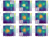 |
Fig. A.1 Target pixel file (TPF) for TOI-375 sectors; the target stars are marked as a white cross on top of a red point, and are indicated by the number 1. The smaller red points are the closest stars to the target (drawn from Gaia) with Gaia magnitude differences with the target of |∆G| < 6. There are no nearby sources of contamination for TOI-375. The plot was made using tpfplotter (Aller et al. 2020). |
Comparison of different radial velocity models.
Complete set of priors used in the juliet runs and their corresponding posterior distributions.
All Tables
Complete set of priors used in the juliet runs and their corresponding posterior distributions.
All Figures
|
Fig. 1 Position of TOI-375 in the HR diagram (black star), using the stellar parameters derived here (see Table 3). For comparison, the position of known giant stars hosting transiting giant planets are overplotted. Two different PARSEC models (Bressan et al. 2012) for 1.0 and 1.45 M⊙, are overplotted. The solid and dotted lines correspond to Z* =0.017 and 0.020, respectively. |
| In the text | |
|
Fig. 2 Speckle autocorrelation function for TOI-375, obtained with the SOAR telescope. The black dots represent the 5σ contrast curve, and the solid line shows a linear fit to the data at separations smaller and larger than ~0.2 arcsec. |
| In the text | |
|
Fig. 3 Periodogram of the radial velocities (top) and activity indices (middle), along with the window function of the observations (bottom) for the FEROS data of TOI-375. False-alarm probabilities are indicated by horizontal lines: dashed red for 1% FAP and dotted blue for 0.1% FAP in each panel. The green vertical lines mark peaks in the radial-velocity periodogram with a FAP below 1% or corresponding to a confirmed a priori planetary signal, such as the 9.4-day signal. In contrast, the magenta vertical lines indicate signals that are unlikely to be of planetary origin. |
| In the text | |
|
Fig. 4 Phase-folded light curves (in green) from each instrument (or sector in the case of TESS) with the best-fit transit model for TOI-375 b derived using juliet. Also shown is the potential single transit event (in blue) of one of the outer planets on TESS sector 2. Data points are shown in their original time sampling (small green or blue points) and binned in phase with 6 minute intervals (white markers). The solid black line represents the best-fit transit model. We do not include the transit of TOI-375 c in the final model as there is not enough evidence to support that it has a true planetary origin. |
| In the text | |
|
Fig. 5 Top : radial velocities along with the median model (black line) for TOI-375. Our model is composed of three different Keplerian components. Bottom : Keplerian components of the full model presented in the top panel. The 9.4-day variation is from TOI-375 b, the transiting exoplanet detected by TESS. The two additional 118.7 and 289.9-day signals observed in our radial-velocities have been identified as likely candidate exoplanets (c and d) given no obvious stellar activity origin. |
| In the text | |
|
Fig. 6 Top : transit timing residuals (∆T) as a function of time for TOI-375 b. ∆T represents the observed transit times minus the calculated times from the linear ephemeris of the joint model. Bottom : Lomb-Scargle periodogram of the TTV signal. |
| In the text | |
|
Fig. 7 Systems with three or more planets in the mass range 0.3 MJ < M < 30 MJ. Planets shown with a cross lack radius measurements, and the mass used corresponds to the minimum mass (Msin(i)). TOI-375 represents the second ever discovery of a multi-Jupiter-mass system where at least one planet’s transit has been detected. |
| In the text | |
|
Fig. 8 Metal enrichment as a function of mass for gas giants. The mass-metallicity trend and sample data are provided by (T16 Thorngren et al. 2016). |
| In the text | |
|
Fig. 9 Position of TOI-375 b in the age-radius diagram (black dot) and planet evolutionary models with core masses of 28, 49, and 49 M⊕. |
| In the text | |
|
Fig. 10 Equilibrium temperature as a function of the system age (solid line), computed using the closest model in the PARSEC grid (M* = 1.45 M⊙; Z* = 0.20; see Fig. 1). The position of TOI-375 b is overplotted (black dot). |
| In the text | |
|
Fig. A.1 Target pixel file (TPF) for TOI-375 sectors; the target stars are marked as a white cross on top of a red point, and are indicated by the number 1. The smaller red points are the closest stars to the target (drawn from Gaia) with Gaia magnitude differences with the target of |∆G| < 6. There are no nearby sources of contamination for TOI-375. The plot was made using tpfplotter (Aller et al. 2020). |
| In the text | |
Current usage metrics show cumulative count of Article Views (full-text article views including HTML views, PDF and ePub downloads, according to the available data) and Abstracts Views on Vision4Press platform.
Data correspond to usage on the plateform after 2015. The current usage metrics is available 48-96 hours after online publication and is updated daily on week days.
Initial download of the metrics may take a while.