| Issue |
A&A
Volume 706, February 2026
|
|
|---|---|---|
| Article Number | L11 | |
| Number of page(s) | 5 | |
| Section | Letters to the Editor | |
| DOI | https://doi.org/10.1051/0004-6361/202557598 | |
| Published online | 10 February 2026 | |
Letter to the Editor
Does the solar oxygen abundance change over the solar cycle?
An investigation into activity-induced variations in the O I infrared triplet
1
Leibniz-Institut für Astrophysik Potsdam (AIP) An der Sternwarte 16 14482 Potsdam, Germany
2
ESO – European Southern Observatory, Alonso de Cordova 3107 Vitacura Santiago, Chile
★ Corresponding author: This email address is being protected from spambots. You need JavaScript enabled to view it.
Received:
8
October
2025
Accepted:
22
January
2026
Abstract
The determination of the solar oxygen abundance remains a central problem in astrophysics because its accuracy is limited not only by models, but also by systematics. While many of these factors have been thoroughly characterized, the effect of the solar activity cycle has remained unexplored so far. Because of its relative strength and accessibility, the O I infrared triplet is typically the primary choice for abundance studies. Previous investigations have shown, however, that abundances inferred from this triplet tend to be higher than expected on active stars, but no such overabundance effect is observed for the much weaker forbidden O I 6300 Å line. This raises the question of whether a similar trend can be found for the Sun. To address this question, we analyzed synoptic disk-integrated Sun-as-a-star datasets of two decades from the FEROS, HARPS-N, PEPSI, and NEID spectrographs with a focus on the infrared triplet (7772, 7774, and 7775 Å) and the forbidden O I 6300 Å line. The excellent signal-to-noise ratio of the PEPSI observations allowed us to detect a weak but significant variation in the equivalent widths of the infrared triplet that corresponds to an abundance difference of about 0.01 dex between activity minimum and maximum. This value is significantly lower than the typical uncertainties on the solar oxygen abundance. No comparable trend is found in the other datasets because the scatter is higher. Based on these results, we conclude that within the typical uncertainties presented in other works, we can assume the inferred solar oxygen abundance to be stable throughout the solar cycle, but that this effect might be significant for other more active stars.
Key words: atomic data / radiative transfer / techniques: spectroscopic / Sun: abundances / Sun: photosphere
© The Authors 2026
 Open Access article, published by EDP Sciences, under the terms of the Creative Commons Attribution License (https://creativecommons.org/licenses/by/4.0), which permits unrestricted use, distribution, and reproduction in any medium, provided the original work is properly cited.
This article is published in open access under the Subscribe to Open model. This email address is being protected from spambots. You need JavaScript enabled to view it. to support open access publication.
1. Introduction
The solar oxygen abundance1, A(O), is a fundamental reference point in astrophysical processes, such as the galaxy metallicity (e.g. Zabel et al. 2021; Le Reste et al. 2022), stellar evolution (e.g., VandenBerg et al. 2012), and the formation properties of exoplanets (e.g., Line et al. 2021). Additionally, its abundance strongly affects the opacity of stellar interiors, and it is thus an important ingredient in stellar models and evolution codes (e.g., Basu & Antia 2008; Bergemann et al. 2021). It is thus crucial to accurately constrain the A(O).
This has been the focus of many studies over the past forty years (Lind & Amarsi 2024, Fig. 7). Differences are still found when the derived abundance for different datasets is compared, however. For example, several observations from different sources were studied by Bergemann et al. (2021) and later by Pietrow et al. (2023). All were processed in the same way, but the inferred values have a scatter of just below 0.1 dex. These discrepancies are generally attributed to instrumental effects such as fringing, continuum placement, and resolution, and to uncertainties in atomic data, including oscillator strengths, line blends, and collisional rates. An additional factor that has not yet been investigated is the possibility of activity-induced spectral line variations over the solar cycle. This is particularly relevant since most A(O) studies have been based on data taken during the solar maximum and the declining phase (see Fig. 1).
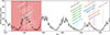 |
Fig. 1. Monthly mean sunspot number (black line) showing the last six solar cycles. The shaded bands indicate the windows used for observing in previous solar oxygen abundance studies. These windows are labeled according to their color. |
This potential correlation may not have been investigated for oxygen specifically because of the influential study by Livingston et al. (2007), who showed that weak photospheric lines forming in the lower photosphere, such as carbon C I 5380 Å, do not vary over the solar cycle (e.g., Al Moulla et al. 2022). In contrast, strong lines forming in the upper photosphere, such as the Na I D doublet, exhibited clear correlations with solar activity. While it is generally agreed that these differences reflect activity-related biases in the equivalent width (EW) of spectral lines and not true changes in elemental abundances (Yana Galarza et al. 2019; Baratella et al. 2020a; Spina et al. 2020), a definitive explanation is still lacking. It is especially important to resolve this issue because most stellar abundance measurement techniques do not explicitly account for activity effects (although some solutions are being investigated; e.g., Nordlander et al. 2024).
Nevertheless, the effect of the solar cycle on A(O) has not yet been investigated to our knowledge, although several indicators suggest it might be relevant. For example, Morel & Micela (2004) found that abundances obtained from the infrared oxygen triplet tended to be higher for more active stars, while no such correlation was found for the lower-forming forbidden O I 6300 Å line. This result was later confirmed by Schuler et al. (2006) and Shen et al. (2007). This effect was also noted in galactic abundance studies, although this difference was not attributed to activity, but atmospheric parameters (e.g. Fabbian et al. 2009).
A similar trend has been reported on young and active stars for other elements, including C I and chromium Cr II (Baratella et al. 2020b), and most notably, barium (Ba, Reddy & Lambert 2017; Baratella et al. 2021). Using solar data, Pietrow et al. (2024) attempted to detect changes in photospheric abundances by analyzing Sun-as-a-star spectra during a strong flare. No measurable variation was found, however. Hanassi-Savari et al. (2025) reported EW changes in various solar spectral lines between the solar minimum and maximum, however.
In this Letter, we use four independent long-term synoptic solar datasets to investigate whether the solar oxygen abundance inferred from the O I infrared triplet and the forbidden O I 6300 Å line exhibit measurable variations over the solar cycle.
2. Observations and data processing
This study makes use of four Sun-as-a-star datasets, each covering a significant part of a solar cycle. The details and location of each instrument are given below. All signal-to-noise ratios (S/Ns) are given per pixel and are measured around 5500 Å.
2.1. FEROS
The Fiber-fed Extended Range Optical Spectrograph (FEROS, Kaufer et al. 1997) is mounted on the ESO 2.2 m telescope in the La Silla observatory in Chile. It has a spectral resolution of ℛ ≈ 48000 and a bandpass between 3500 and 9200 Å. From November 2003 to May 2011, the instrument had a daily SolarSpectrum program in which the telescope took scattered-light solar calibration spectra by pointing 30 degrees from the Sun. This was done as a workaround for the halogen calibration lamps, which were too weak in the blue. Unfortunately, these observations ceased after the instrument was upgraded with new calibration lamps in 2011 (François 2016). The spectra have an S/N of 200 on average. The data are available in the ESO archive2 under the program id 60.A-9700.
2.2. HARPS-N
The High Accuracy Radial velocity Planet Searcher in the North (HARPS-N, Cosentino et al. 2012) is a fiber-fed spectrograph mounted on the Galileo National Telescope on La Palma, Spain. It observes the Sun since 2015 via a dedicated 6 mm solar telescope (Dumusque et al. 2015) at a 5-minute cadence. It has a spectral resolution of ℛ ≈ 120000 and simultaneously observes between 3900 and 6900 Å at an S/N of 400. All data from the past decade were recently released on the DACE platform3 (Dumusque et al. 2025).
2.3. PEPSI
The Potsdam Echelle Polarimetric and Spectroscopic Instrument (PEPSI, Strassmeier et al. 2015) is a fiber-fed spectrograph installed at the Large Binocular Telescope on Mt. Graham, Arizona, USA. It observes the Sun since September 2015 through a dedicated 13 mm solar telescope (Strassmeier et al. 2018). It covers the wavelength range from 3830 to 9070 Å with a spectral resolution of up to ℛ ≈ 250000 at an S/N of 1000. The solar feed underwent an upgrade in July 2023 to also observe full Stokes polarimetry, and it resumed operations in June 2024 (Strassmeier et al. 2024). The data are available upon request to the instrument PI.
2.4. NEID
The NN-Explore extreme precision Doppler spectrometer (NEID, Schwab et al. 2016) is a fiber-fed spectrograph mounted on the 3.5 m WIYN telescope at Kitt Peak National Observatory, Arizona, USA. It observes the Sun since December 2020 through a dedicated 75 mm solar telescope (Lin et al. 2022). It has a spectral resolution of ℛ ≈ 110000 over a bandpass from 3800 to 9300 Å, with an average S/N of 320. These data are publicly released through the NEID Solar Archive4.
2.5. Data processing
The data from each telescope were sorted by their S/N, and the highest-quality observations were selected for each month within a three-day window of the 15th, as close to local noon as possible. For FEROS and NEID, a selection was made around the O I infrared triplet. For HARPS-N, this wavelength was outside of the instrument wavelength range, and thus, the O I 6300 Å line was considered instead. All four lines were considered for PEPSI.
3. Methods, results, and discussion
We used the code called automatic routine for line EWs in stellar spectra (ARES v2, Sousa et al. 2015) to measure the EWs of the selected lines. The code automatically fits a Gaussian profile and normalizes the local continuum (Sousa et al. 2007)5. The amplitude of these values was then compared with the spot number6. Additionally, two statistical tests were applied to these data for each line separately. First, we calculated the Pearson correlation coefficient (PCC) for the EW as a function of spot number. Second, we split the data into two populations and took the median. This resulted in (1) an active population with a spot number ≥50, and (2) a quiet population with a spot number < 50.
In Fig. 2 the EWs are plotted over time together with the spot number, which illustrates the solar cycle. In Fig. 3 the EW is plotted against the spot number.
 |
Fig. 2. Measured EW of the O I 7772 Å line with FEROS (blue), PEPSI (orange), and NEID (green), including corresponding uncertainties. The gray curve shows the sunspot number as an activity reference, and the horizontal black line at 50 distinguishes active from quiet times. The corresponding plots for the three remaining lines are shown in Fig. B.1. |
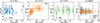 |
Fig. 3. EWs of the O I 7772 Å line for FEROS (blue), PEPSI (orange), and NEID (green) as a function of spot number. The corresponding plots for the three remaining lines are shown in Fig. B.2. |
The results of the PCC, together with the median EWs for both groups, are listed in Table 1 for each instrument and line. The difference between the inferred EW and abundance values is also given, marked with a delta (Δ), along with the standard uncertainties.
Correlation statistics of EWs with solar activity.
To give a rough indication of the significance of these EW differences between active and quiet, we then computed A(O) for the infrared triplet based on a curve-of-growth equation obtained from the 3D NLTE analysis by Steffen et al. (2015), which are given in Appendix A. The difference between the high- and low-abundance values is shown in the same table. No abundance estimate was made for O I 6300 Å line because this line is blended with a Ni I line and requires different modeling.
For the infrared lines, we found that the null hypothesis of the PCC cannot be rejected for either FEROS or NEID, whereas a weak but significant trend appears to be present in the infrared PEPSI EW data. The difference between the high and low median is about 1 mÅ for this instrument. When converted into abundances, this corresponds to a change of about 0.01 dex. This value is below the typical systematic uncertainties of the A(O) computation.
For the forbidden oxygen line, we found no trend in our measurements, which agrees with the findings of Morel & Micela (2004). With our prior abundance change of 0.01 dex, the expected change in EW would be 0.05 mÅ, which is beyond our precision for this weak line.
4. Conclusions
We investigated the EWs of four synoptic Sun-as-a-star datasets, each covering a significant part of a solar cycle. Of these datasets, only the S/N of the PEPSI data was high enough to allow the detection of a weak but statistically significant correlation between the solar cycle and the EW of the O I infrared triplet (see Table 1). The PEPSI and HARPS-N observations of the O I 6300 Å line did not show a trend, likely because the response of this line to activity is weaker by an order of magnitude and because the instrument precision is limited.
To illustrate the impact of these changes in EW, we converted them into A(O) values based on the 3D NLTE calculations of Steffen et al. (2015). We found a small but consistent change of about 0.01 dex in the PEPSI spectra. This value is well below the typical uncertainties of published A(O) values (see Fig. 7 in Lind & Amarsi 2024, and the discussions in Bergemann et al. 2025 and Lodders et al. 2025) and is therefore not relevant for the determination of the solar O(A), but larger activity imprints would amplify this effect, as was shown for younger (see the effects on A(O) in the 600 Myr Hyades dwarf stars; Schuler et al. 2006) and more active stars (e.g., for log R′HK > −4.3 Morel & Micela 2004).
This finding, together with the fact that other stars can exhibit much stronger activity levels, suggests that this might represent a significant source of bias in abundance determinations for younger stars. The high S/N of the PEPSI observations was crucial for detecting this subtle trend. Future work will investigate the amplitude of this effect in more active solar analogs and through synthetic Sun-as-a-star spectra with controlled activity-filling factors using the Numerical Empirical Sun-as-a-Star Integrator (NESSI, Pietrow & Pastor Yabar 2024).
Acknowledgments
AP was supported by grant PI 2102/1-1 from the Deutsche Forschungsgemeinschaft (DFG) and gratefully acknowledges the ESO Chile Scientific Visitor Programme.
References
- Al Moulla, K., Dumusque, X., Cretignier, M., Zhao, Y., & Valenti, J. A. 2022, A&A, 664, A34 [NASA ADS] [CrossRef] [EDP Sciences] [Google Scholar]
- Allende Prieto, C., Lambert, D. L., & Asplund, M. 2001, ApJ, 556, L63 [Google Scholar]
- Amarsi, A. M., Barklem, P. S., Asplund, M., Collet, R., & Zatsarinny, O. 2018, A&A, 616, A89 [NASA ADS] [CrossRef] [EDP Sciences] [Google Scholar]
- Amarsi, A. M., Grevesse, N., Asplund, M., & Collet, R. 2021, A&A, 656, A113 [NASA ADS] [CrossRef] [EDP Sciences] [Google Scholar]
- Anders, E., & Grevesse, N. 1989, Geochim. Cosmochim. Acta, 53, 197 [Google Scholar]
- Asplund, M., Grevesse, N., Sauval, A. J., Allende Prieto, C., & Kiselman, D. 2004, A&A, 417, 751 [NASA ADS] [CrossRef] [EDP Sciences] [Google Scholar]
- Asplund, M., Grevesse, N., Sauval, A. J., & Scott, P. 2009, ARA&A, 47, 481 [NASA ADS] [CrossRef] [Google Scholar]
- Asplund, M., Amarsi, A. M., & Grevesse, N. 2021, A&A, 653, A141 [NASA ADS] [CrossRef] [EDP Sciences] [Google Scholar]
- Baratella, M., D’Orazi, V., Carraro, G., et al. 2020a, A&A, 634, A34 [NASA ADS] [CrossRef] [EDP Sciences] [Google Scholar]
- Baratella, M., D’Orazi, V., Biazzo, K., et al. 2020b, A&A, 640, A123 [NASA ADS] [CrossRef] [EDP Sciences] [Google Scholar]
- Baratella, M., D’Orazi, V., Sheminova, V., et al. 2021, A&A, 653, A67 [NASA ADS] [CrossRef] [EDP Sciences] [Google Scholar]
- Basu, S., & Antia, H. M. 2008, Phys. Rep., 457, 217 [Google Scholar]
- Bergemann, M., Hoppe, R., Semenova, E., et al. 2021, MNRAS, 508, 2236 [NASA ADS] [CrossRef] [Google Scholar]
- Bergemann, M., Lodders, K., & Palme, H. 2025, ArXiv e-prints [arXiv:2503.05402] [Google Scholar]
- Bertello, L., Pevtsov, A., Tlatov, A., & Singh, J. 2016, Sol. Phys., 291, 2967 [NASA ADS] [CrossRef] [Google Scholar]
- Caffau, E., Steffen, M., & Ludwig, H. G. 2008, Eur. Sol. Phys. Meet., 12, 3.7 [NASA ADS] [Google Scholar]
- Caffau, E., Ludwig, H. G., Steffen, M., et al. 2015, A&A, 579, A88 [NASA ADS] [CrossRef] [EDP Sciences] [Google Scholar]
- Clette, F., Berghmans, D., Vanlommel, P., et al. 2007, Adv. Space Res., 40, 919 [NASA ADS] [CrossRef] [Google Scholar]
- Clette, F., Svalgaard, L., Vaquero, J. M., & Cliver, E. W. 2015, in The Solar Activity Cycle, eds. A. Balogh, H. Hudson, K. Petrovay, & R. von Steiger, 53, 35 [Google Scholar]
- Cosentino, R., Lovis, C., Pepe, F., et al. 2012, SPIE Conf. Ser., 8446, 84461V [Google Scholar]
- Cretignier, M., Pietrow, A. G. M., & Aigrain, S. 2024, MNRAS, 527, 2940 [Google Scholar]
- Cubas Armas, M., Asensio Ramos, A., & Socas-Navarro, H. 2020, A&A, 643, A142 [NASA ADS] [CrossRef] [EDP Sciences] [Google Scholar]
- Dumusque, X., Glenday, A., Phillips, D. F., et al. 2015, ApJ, 814, L21 [Google Scholar]
- Dumusque, X., Al Moulla, K., Cretignier, M., et al. 2025, The HARPS-N Solar Telescope Legacy: A decade of Solar High-Fidelity Spectroscopy and Precise Radial Velocities [Google Scholar]
- Fabbian, D., Asplund, M., Barklem, P. S., Carlsson, M., & Kiselman, D. 2009, A&A, 500, 1221 [NASA ADS] [CrossRef] [EDP Sciences] [Google Scholar]
- François, P. 2016, FEROS-II User Manual, Version 78.0, https://www.eso.org/sci/facilities/lasilla/instruments/feros/doc/manual/P78/FEROSII-UserManual-78.0.pdf, European Southern Observatory, La Silla 2.2m Telescope [Google Scholar]
- Grevesse, N., & Sauval, A. J. 1998, Space Sci. Rev., 85, 161 [Google Scholar]
- Grevesse, N., Asplund, M., & Sauval, A. J. 2007, Space Sci. Rev., 130, 105 [Google Scholar]
- Hanassi-Savari, F., Pietrow, A. G. M., Druett, M. K., Cretignier, M., & Ellwarth, M. 2025, A&A, 702, A97 [NASA ADS] [CrossRef] [EDP Sciences] [Google Scholar]
- Kaufer, A., Wolf, B., Andersen, J., & Pasquini, L. 1997, Messenger, 89, 1 [NASA ADS] [Google Scholar]
- Le Reste, A., Hayes, M., Cannon, J. M., et al. 2022, ApJ, 934, 69 [NASA ADS] [CrossRef] [Google Scholar]
- Lin, A. S. J., Monson, A., Mahadevan, S., et al. 2022, AJ, 163, 184 [NASA ADS] [CrossRef] [Google Scholar]
- Lind, K., & Amarsi, A. M. 2024, ARA&A, 62, 475 [NASA ADS] [CrossRef] [Google Scholar]
- Line, M. R., Brogi, M., Bean, J. L., et al. 2021, Nature, 598, 580 [NASA ADS] [CrossRef] [Google Scholar]
- Livingston, W., Wallace, L., White, O. R., & Giampapa, M. S. 2007, ApJ, 657, 1137 [CrossRef] [Google Scholar]
- Lodders, K., Bergemann, M., & Palme, H. 2025, Space Sci. Rev., 221, 23 [Google Scholar]
- Magg, E., Bergemann, M., Serenelli, A., et al. 2022, A&A, 661, A140 [NASA ADS] [CrossRef] [EDP Sciences] [Google Scholar]
- Morel, T., & Micela, G. 2004, A&A, 423, 677 [NASA ADS] [CrossRef] [EDP Sciences] [Google Scholar]
- Nordlander, T., Baratella, M., Spina, L., & D’Orazi, V. 2024, MNRAS, 535, 2863 [Google Scholar]
- Pietrow, A. G. M., & Pastor Yabar, A. 2024, IAU Symp., 365, 389 [NASA ADS] [Google Scholar]
- Pietrow, A. G. M., Hoppe, R., Bergemann, M., & Calvo, F. 2023, A&A, 672, L6 [NASA ADS] [CrossRef] [EDP Sciences] [Google Scholar]
- Pietrow, A. G. M., Cretignier, M., Druett, M. K., et al. 2024, A&A, 682, A46 [NASA ADS] [CrossRef] [EDP Sciences] [Google Scholar]
- Reddy, A. B. S., & Lambert, D. L. 2017, ApJ, 845, 151 [Google Scholar]
- Sauval, A. J., Grevesse, N., Zander, R., Brault, J. W., & Stokes, G. M. 1984, ApJ, 282, 330 [Google Scholar]
- Schuler, S. C., King, J. R., Terndrup, D. M., et al. 2006, ApJ, 636, 432 [Google Scholar]
- Schwab, C., Rakich, A., Gong, Q., et al. 2016, SPIE Conf. Ser., 9908, 99087H [NASA ADS] [Google Scholar]
- Shen, Z. X., Liu, X. W., Zhang, H. W., Jones, B., & Lin, D. N. C. 2007, ApJ, 660, 712 [Google Scholar]
- Socas-Navarro, H. 2015, A&A, 577, A25 [NASA ADS] [CrossRef] [EDP Sciences] [Google Scholar]
- Sousa, S. G., Santos, N. C., Israelian, G., Mayor, M., & Monteiro, M. J. P. F. G. 2007, A&A, 469, 783 [NASA ADS] [CrossRef] [EDP Sciences] [Google Scholar]
- Sousa, S. G., Santos, N. C., Adibekyan, V., Delgado-Mena, E., & Israelian, G. 2015, A&A, 577, A67 [NASA ADS] [CrossRef] [EDP Sciences] [Google Scholar]
- Spina, L., Nordlander, T., Casey, A. R., et al. 2020, ApJ, 895, 52 [Google Scholar]
- Steffen, M., Prakapavičius, D., Caffau, E., et al. 2015, A&A, 583, A57 [NASA ADS] [CrossRef] [EDP Sciences] [Google Scholar]
- Strassmeier, K. G., Ilyin, I., Järvinen, A., et al. 2015, Astron. Nachr., 336, 324 [NASA ADS] [CrossRef] [Google Scholar]
- Strassmeier, K. G., Ilyin, I., & Steffen, M. 2018, A&A, 612, A44 [NASA ADS] [CrossRef] [EDP Sciences] [Google Scholar]
- Strassmeier, K. G., Ilyin, I., Woche, M., et al. 2024, Astron. Nachr., 345, e20240033 [NASA ADS] [CrossRef] [Google Scholar]
- VandenBerg, D. A., Bergbusch, P. A., Dotter, A., et al. 2012, ApJ, 755, 15 [Google Scholar]
- Yana Galarza, J., Meléndez, J., Lorenzo-Oliveira, D., et al. 2019, MNRAS, 490, L86 [Google Scholar]
- Zabel, N., Davis, T. A., Smith, M. W. L., et al. 2021, MNRAS, 502, 4723 [NASA ADS] [CrossRef] [Google Scholar]
We adopted the traditional astronomical logarithmic abundance scale A(O) = 12 + log10(nO/nH), which expresses the abundance of oxygen on a logarithmic scale relative to nH = 1012 hydrogen atoms.
The EWs reported here are slightly underestimated, as the lines deviate from a purely Gaussian profile and their extended wings are not fully included in the integration (See also footnote 7).
The spot number (Clette et al. 2007, 2015) is defined as R = k(10g + s), with g the number of groups, s the number of spots, and k a scaling factor depending on the observatory. This metric has been shown to track the Ca II H&K based S-index (e.g. Bertello et al. 2016), even though the Sun is dominated by plages (e.g. Cretignier et al. 2024).
The EW of the oxygen triplet lines given in Steffen et al. (2015) are somewhat larger than found in the present work because they were derived from synthetic spectra and include the far wings.
Appendix A: Curve of growth
The following 3D NLTE curves-of-growth are based on the work of Steffen et al. (2015). This study employed a 22-level oxygen model atom, including electron and hydrogen collisions scaled via the SH parameter, which is observationally constrained by the center-to-limb variation of the oxygen triplet. This atom was then used for full 3D non-LTE line formation based on a CO5BOLD hydrodynamical solar model, NLTE3D for the computation of departure coefficients, and Linfor3D for the generation of synthetic spectra.
These curves were used to convert the measured differences in EW7 into corresponding differences of the (logarithmic) oxygen abundance A(O) (with A0 = 8.76):
 (A.1)
(A.1)
 (A.2)
(A.2)
 (A.3)
(A.3)
Appendix B: Further figures
All Tables
All Figures
|
Fig. 1. Monthly mean sunspot number (black line) showing the last six solar cycles. The shaded bands indicate the windows used for observing in previous solar oxygen abundance studies. These windows are labeled according to their color. |
| In the text | |
|
Fig. 2. Measured EW of the O I 7772 Å line with FEROS (blue), PEPSI (orange), and NEID (green), including corresponding uncertainties. The gray curve shows the sunspot number as an activity reference, and the horizontal black line at 50 distinguishes active from quiet times. The corresponding plots for the three remaining lines are shown in Fig. B.1. |
| In the text | |
|
Fig. 3. EWs of the O I 7772 Å line for FEROS (blue), PEPSI (orange), and NEID (green) as a function of spot number. The corresponding plots for the three remaining lines are shown in Fig. B.2. |
| In the text | |
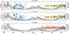 |
Fig. B.1. Same as Fig. 2 but for the remaining IR triplet lines and the forbidden line. |
| In the text | |
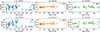 |
Fig. B.2. Same as Fig. 3 but for the remaining lines. |
| In the text | |
Current usage metrics show cumulative count of Article Views (full-text article views including HTML views, PDF and ePub downloads, according to the available data) and Abstracts Views on Vision4Press platform.
Data correspond to usage on the plateform after 2015. The current usage metrics is available 48-96 hours after online publication and is updated daily on week days.
Initial download of the metrics may take a while.