| Issue |
A&A
Volume 706, February 2026
|
|
|---|---|---|
| Article Number | A28 | |
| Number of page(s) | 13 | |
| Section | Stellar structure and evolution | |
| DOI | https://doi.org/10.1051/0004-6361/202557603 | |
| Published online | 27 January 2026 | |
A magnetar outburst with atypical evolution: The case of Swift J1555.2–5402
1
European Space Science (ESA), European Space Astronomy Center (ESAC) Camino Bajo del Castillo s/n E-28692 Villanueva de la Cañada Madrid, Spain
2
Institute of Space Sciences (ICE, CSIC), Campus UAB Carrer de Can Magrans s/n E-08193 Barcelona, Spain
3
Institut d’Estudis Espacials de Catalunya (IEEC) E-08860 Castelldefels (Barcelona), Spain
4
INAF–Osservatorio Astronomico di Brera Via Bianchi 46 Merate (LC) I-23807, Italy
5
INAF–Osservatorio Astronomico di Roma via Frascati 33 I-00078 Monteporzio Catone, Italy
6
INAF–Istituto di Astrofisica Spaziale e Fisica Cosmica di Milano via A. Corti 12 I-20133 Milano, Italy
7
Università degli Studi di Milano Bicocca, Dipartimento di Fisica G. Occhialini Piazza della Scienza 3 I-20126 Milano, Italy
8
INAF–Osservatorio Astronomico di Cagliari Via della Scienza 5 I-09047 Selargius, Italy
9
Scuola Universitaria Superiore IUSS Pavia Piazza della Vittoria 15 I-27100 Pavia, Italy
10
Dipartimento di Fisica e Astronomia, Università degli Studi di Padova via F. Marzolo 8 I-35131 Padova, Italy
11
Mullard Space Science Laboratory, University College London Holmbury St. Mary Dorking Surrey RH5 6NT, UK
12
Institut für Astronomie und Astrophysik, Universität Tübingen Sand 1 D-72076 Tübingen, Germany
★ Corresponding author: This email address is being protected from spambots. You need JavaScript enabled to view it.
Received:
8
October
2025
Accepted:
8
December
2025
Abstract
The magnetar Swift J1555.2–5402 was discovered in outburst on 2021 June 3 by the Burst Alert Telescope on board the Swift satellite. Early X-ray follow-up revealed a spin period P ≃ 3.86 s, a period derivative Ṗ ≃ 3 × 10⁻¹¹ s s−1, dozens of short bursts, and an unusual flux decline. We report here on the X-ray monitoring of Swift J1555.2–5402 over the first ≃29 months of its outburst with Swift, NICER, NuSTAR, INTEGRAL, and Insight-HXMT, as well as radio observations with Parkes soon after the outburst onset. The observed 0.3–10 keV flux remained at levels ≳10−11 erg cm−2 s−1 for nearly 500 days before dropping by a factor of ≃10 from its 2021 June peak towards the end of the monitoring campaign. During this time span, the spectrum was dominated by a single blackbody, whose temperature attained an approximately constant value (∼1.2 keV), while the inferred radius shrank from ≈1.7 km to ≈0.3 km (assuming a source distance of 10 kpc). The long-term spin-down rate (Ṗ ≃ 3.6 × 10⁻¹¹ s s−1) is only ∼15% higher than that measured in the first 30 days. No periodic or burst-like radio emission was detected, in line with what had been previously reported using different radio facilities. The persistently high temperature, shrinking hotspot, and prolonged bright flux plateau followed by a fast dimming observed during the outburst evolution pose a challenge for the outburst mechanisms proposed so far.
Key words: stars: magnetars / stars: magnetic field / stars: neutron / pulsars: general / X-rays: bursts
ESA Research Fellow.
© The Authors 2026
 Open Access article, published by EDP Sciences, under the terms of the Creative Commons Attribution License (https://creativecommons.org/licenses/by/4.0), which permits unrestricted use, distribution, and reproduction in any medium, provided the original work is properly cited.
This article is published in open access under the Subscribe to Open model. This email address is being protected from spambots. You need JavaScript enabled to view it. to support open access publication.
1. Introduction
Magnetars are isolated X-ray pulsars with luminosity LX ∼ 1031–1036 erg s−1 whose emission is believed to be powered by the dissipation of their magnetic energy (for reviews, see Turolla et al. 2015; Kaspi & Beloborodov 2017; Esposito et al. 2021; Rea & De Grandis 2025). Their most spectacular observational manifestations are bursts of X-rays and/or gamma-rays and X-ray outbursts. The former are observed on timescales from milliseconds to minutes, reaching peak luminosities LX ∼ 1038–1046 erg s−1 (e.g. Collazzi et al. 2015). The latter are longer-lived episodes where the persistent luminosity increases by a factors of few to thousands up to LX ∼ 1034–1036 erg s−1 and then usually decreases back to quiescence on timescales of months to years (see e.g. the Magnetar Outburst Online Catalog1; Coti Zelati et al. 2018). The onset of an outburst is typically accompanied by and discovered through the emission of short bursts. The decay pattern differs from outburst to outburst, but it is often characterised by a rapid initial decay within hours to a few days, followed by a slower fading that can be modelled by a power law or exponential functions. Despite the great diversity in decay profiles, all outbursts share some common trends. For instance, a higher luminosity at the outburst onset typically corresponds to a larger amount of energy released during the entire event (generally in the range ∼1041 − 1043 erg), and outbursts with a longer overall duration tend to be the most energetic ones (Coti Zelati et al. 2018). Outbursts are most likely caused by a sudden release of heat in a restricted area within or just above the magnetar crust, leading to the formation of a hot spot that progressively cools down. However, the exact triggering mechanism is still an open question: it may involve localised internal magnetic stresses that deform part of the crust (see e.g. Dehman et al. 2020; De Grandis et al. 2022) or a twisted bundle in the magnetosphere (see e.g. Beloborodov 2009; Carrasco et al. 2019).
Swift J1555.2–5402 (hereafter Sw J1555) was discovered on 2021 June 3 at 09:45:46 UT, when the Burst Alert Telescope (BAT) on board the Neil Gehrels Swift Observatory (Swift) triggered and localised a short burst of X-rays similar to those emitted by magnetars (Palmer et al. 2021). Over the following hours, an X-ray counterpart was discovered using the Swift X-ray Telescope (XRT) and a periodic modulation of its X-ray emission with P∼3.86 s was measured using the Neutron star Interior Composition Explorer (NICER). This confirmed the magnetar nature of the source (Coti Zelati et al. 2021b). NICER observed Sw J1555 with a daily cadence over the first month of its outburst, revealing a thermal spectrum at a nearly constant flux of ∼4 × 10⁻¹¹ erg cm−2 s−1 in the soft X-ray band throughout this time span. Emission up to energies of ∼40 keV with a spectral shape well described by a power law was also detected using the Nuclear Spectroscopic Telescope Array (NuSTAR). The NICER observations allowed a measurement of the spin period derivative, Ṗ ≃ 3 × 10⁻¹¹ s s−1, and also revealed a number of bursts from the source (Enoto et al. 2021; see also Bernardini et al. 2021; Klingler et al. 2021; Zhang et al. 2021).
This paper presents X-ray observations of Sw J1555 using NICER, Swift/XRT, Insight-HXMT, NuSTAR, and INTEGRAL over the first 29 months of the outburst, as well as radio observations performed using Parkes soon after the outburst onset (Sect. 2). We report on (i) the X-ray spectral and timing properties of Sw J1555 (Sects. 3.1, 3.2 and 3.3) and on the results of our searches for short X-ray bursts (Sect. 3.4), and (ii) searches for periodic and/or bursting radio emission in observations with Parkes/Murriyang close to the peak of the outburst (Sect. 3.5). A discussion of the results and conclusions is presented in Sect. 4.
2. Observations and data analysis
2.1. X-ray observations
Table A.1 reports the log of the X-ray observations used in this work. Additional NICER and NuSTAR observations were carried out during the first month of the outburst, and were analysed by Enoto et al. (2021).
The data reduction was performed with tools provided in HEASOFT (v.6.33) and HXMTDAS (v.2.06). Photon arrival times were barycentred using the Swift/XRT enhanced position, RA = 15h55m08 66, Dec = –54°03′41
 1 (J2000.0; uncertainty of 2.2″ at 90% c.l.; Evans 2021) and the JPL planetary ephemeris DE430. The spectral analysis was performed using XSPEC (Arnaud 1996), applying the TBABS model with cross-sections of Verner et al. (1996) and elemental abundances of Wilms et al. (2000) to describe the effects of interstellar absorption and the convolution model CFLUX to estimate the source flux. In the following, we quote all uncertainties at a 1σ confidence level (c.l.) and assume a distance to the source of 10 kpc.
2.1.1. Swift
The Swift/XRT (Burrows et al. 2005) monitored Sw J1555 with 85 pointings between 2021 June 3 and 2023 October 21. Most observations were performed with the XRT in the windowed timing mode (WT; time resolution of 1.8 ms) to study the time evolution of the spin signal. Five sparse observations between 2021 June 3 and 2022 January 5 and all observations since 2022 mid-August2 were performed instead in photon counting mode (PC; 2.5 s). We collected source photons within a circle with a radius of 20 pixels (1 pixel = 2 36) and background counts from an annulus with radii of 80 and 120 pixels for data in the WT mode and 40 and 80 pixels for data in PC mode. For the spectral analysis, we selected events with grades 0–12 and 0 for PC and WT data, respectively, while we extended the timing analysis to events with grade 0–2 for WT datasets.
The Swift/XRT background-subtracted spectra were grouped to have at least ten counts in each spectral channel up to observation ID 00014971022. Due to the low photon counting statistics, in the following observations we opted to bin the remaining Swift spectra according to a variable minimum number of counts between five and three counts per spectral bin. The W-statistic was employed for model parameter estimation and error calculation for all Swift/XRT spectra.
2.1.2. NICER
NICER (Gendreau et al. 2012) observed the field of Sw J1555 for ∼2.5 ks starting on 2021 June 3 at 11:20 UT, just ∼1.6 h after the first Swift/BAT trigger. The source was subsequently monitored over a time interval of ∼4.5 months until 2021 October 22, just before entering a solar constraint period. A dozen additional observations were performed between 2022 July 21 and 2022 August 17. For this work, we only included the data we obtained through our own Target of Opportunity requests (see Table A.1 for a log of the observations). We processed and screened the data using the NICERL2 tool. Then, we extracted background-subtracted spectra and light curves using the NICERL3-SPECT and NICERL3-LC tools, respectively, with the SCORPEON background model3. The spectra were binned to guarantee at least 100 background-subtracted counts per energy bin so as to apply the χ2 statistics.
2.1.3. NuSTAR
Sw J1555 was observed by NuSTAR (Harrison et al. 2013) at four epochs. We report here on the last observation performed on 2021 October 7 (see Enoto et al. 2021, for details on the first three pointings). We applied standard analysis threads to reprocess the raw data for the two focal plane detectors, referred to as focal plane module A and B (FPMA and FPMB). We used the tool OPTIMIZE_RADIUS_SNR of the NuSTAR-gen-utils package (Grefenstette et al. 2025) to estimate the source extraction radius that maximises the S/N. This resulted in circular source extraction regions with radii of 79 arcsec for FPMA and 74 arcsec for FPMB. Background counts were accumulated from a nearby source-free circular region with 70 arcsec radius. We then generated light curves, background-subtracted spectra and response files for both FPMs with the script NUPRODUCTS. We rebinned the data with FTGROUPPHA following the Kaastra & Bleeker optimal binning algorithm (Kaastra & Bleeker 2016) in order to have at least 25 counts per bin. The source was detected up to ∼20 keV at a net count rate of ∼1.34 counts s−1 (summing the two FPMs).
2.1.4. Insight-HXMT
The Hard X-ray Modulation Telescope (Insight-HXMT; Zhang et al. 2020) observed Sw J1555 for ∼100 ks starting on 2021 June 10 at 17:38:32 UT, using the low energy telescope (LE), the medium energy telescope (ME), and the high energy telescope (HE). We used the HPIPELINE to process and screen the data, to create response files, and to extract background-subtracted spectra and light curves. Sw J1555 was detected at a very low signal-to-noise ratio in these data. The LE data alone were used for the analysis, only to refine our timing solution (see Table A.1 for the corresponding on-source exposure time and net count rate after data screening).
2.1.5. INTEGRAL
The position of Sw J1555 was extensively covered by observations with the Imager on board the INTEGRAL Satellite (IBIS; Ubertini et al. 2003). We selected all the science windows4 (ScWs) in the public archive where the source was located within 14.5° from the centre of the IBIS field of view. The selected ScWs were screened for high or variable background. The filtering resulted in a total of 11120 ScWs, corresponding to an observation time of 24.65 Ms before the outburst (from 2003 March to 2021 June 3) and 1.96 Ms divided into 806 ScWs since the outburst onset up to 2023 August 27.
During the first 150 days after the Swift/BAT trigger, INTEGRAL observed the source in the central field of view for 58.8 ks. Using OSA (v.11.2; Goldwurm et al. 2003), we created an image in the 30–80 keV energy interval using all available observations during this period. The source was not detected; we estimate a 3σ upper limit on its flux of 9.7 × 10⁻¹¹ erg cm−2 s−1.
2.2. Radio observations
Three visits were performed using the Ultra Wideband Low-frequency receiver (UWL; Hobbs et al. 2020) of the 64 m Parkes Murriyang Radio telescope (Table A.2). The data were collected with two backends in parallel. The Medusa backend (Hobbs et al. 2020) was always operated over a 3.3 GHz bandwidth centred at 2.4 GHz, with a frequency resolution of 1 MHz, a sampling time of 128 μs, and a 2 bit digitisation. On 2021 June 4 and 7, the PDFB4 backend acquired 256 MHz of data centred at a frequency of 1369 MHz, with a frequency resolution of 0.5 MHz. On 2021 June 5, data were recorded over a 1024 MHz bandwidth, centred at 3100 MHz, with a frequency resolution of 2 MHz. In all cases, the PDFB4 time series were 2 bit sampled every 256 μs.
3. Results
3.1. X-ray monitoring
We fitted an absorbed blackbody to the available NICER and Swift/XRT spectra jointly, tying the hydrogen column density NH among the different datasets and allowing the other parameters to vary. The fit gave an overall satisfactory description of the data with NH = (8.4 ± 0.2) × 1022 cm−2 (null hypothesis probability5 = 0.5). Figure 1 shows the temporal evolution of the temperature and radius of the emitting region, and of the observed and unabsorbed flux in the 0.3–10 keV energy interval. The blackbody temperature kTBB did not display any significant variability during the duration of our monitoring campaign, attaining an average value of ∼1.2 keV. The corresponding radius RBB slowly decreased from ∼1.7 km to ∼0.3 km over ∼895 days, and its temporal evolution can be approximated as an exponential function with an e-folding time of τ = 538 ± 21 days; (chi-square χ2 = 189 for 79 degrees of freedom, d.o.f.). The observed 0.3–10 keV flux gradually decreased from ∼5 × 10⁻¹¹ erg cm−2 s−1 to ∼1 × 10⁻¹¹ erg cm−2 s−1 during the first ∼500 days of our monitoring campaign. Then, a sharper decline followed, with the flux dropping to ∼9 × 10⁻¹³ erg cm−2 s−1 on 2023 October 21 (the epoch of the last observation included in this campaign). The temporal evolution of the observed flux can be described by an exponential function with an e-folding time of τ = 262 ± 3 days. Although the fit does not yield a statistically acceptable result (χ2 = 402 for 79 d.o.f.), this model adequately captures the general trend of the decay. We attribute the high χ2 obtained to the scatter in the data points and/or small-amplitude variability superimposed on the exponential decay. It is worth noting that the decay time of the flux is in agreement with the characteristic time for the radius shrinking assuming blackbody emission at constant temperature.
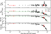 |
Fig. 1. Temporal evolution of the blackbody temperature and radius, and of the observed and unabsorbed flux (0.3–10 keV) of Swift J1555.2–5402 over a time span of about 900 days since the epoch of the first Swift/BAT trigger (on 2021 June 3 at 09:45:46 UT; 59368.40678 MJD). The green dashed lines indicate the fit with an exponential function for the radius and observed flux. |
The sky position of Sw J1555 was serendipitously observed with Swift/XRT a few times before 2021 June. The source was not detected in any observations with a 3σ upper limit on the averaged count rate of 0.007 counts s−1, derived from the stacking of the available archival pointings (see Table A.1). Using the WEBPIMMS tool6 and assuming an absorbed blackbody with NH = 8.4 × 1022 cm−2 and kT = 0.3 keV, the upper limit translates to a 0.3–10 keV observed flux of < 2.7 × 10⁻¹³ erg cm−2 s−1, which corresponds to a luminosity of < 1035 erg s−1 at 10 kpc.
We inspected the observations performed after a burst trigger for the presence of diffuse emission around the source, which may be associated with a rapidly evolving component causally connected with the burst emission, such as a dust scattering halo (see e.g. Tiengo et al. 2010; Mereghetti et al. 2020). Our searches did not yield significant detection.
3.2. Broad-band spectrum
We analysed the broad-band spectrum of the source using the latest NuSTAR observation, jointly fitted with the Swift/XRT spectrum obtained simultaneously (OsbID: 00014352040). The spectral fitting was limited to energies below 20 keV, where the source count rate exceeds the background level. For the spectral analysis, we included a renormalisation factor to account for cross-calibration uncertainties, which was fixed at 1 for NuSTAR/FPMA and allowed to vary for NuSTAR/FPMB and Swift/XRT. A model composed of only an absorbed blackbody did not provide a good fit, and revealed structured residuals above ∼10 keV. The addition of a power law to the model significantly improved the fit to a chi-square χ2 = 210 for 213 d.o.f. The absorption column density was frozen at NH = 8.4 × 1022 cm−2 (see Sect. 3.1). The fit yielded the following values for the constant: 1.00 ± 0.01 for NuSTAR/FPMB and 0.92 ± 0.04 for Swift/XRT. The best-fitting parameters were kTBB = 1.16 ± 0.01 keV,  km, and photon index
  . The parameters for the blackbody component are consistent with those derived from the fitting of the soft X-rays spectra extracted from adjacent observations. The 10 − 60 keV flux was
  erg cm−2 s−1, indicating a ∼20% decrease compared to the previous NuSTAR observation performed three months earlier, which measured a flux of (8.72 ± 0.85)×10−12 erg cm−2 s−1 (Enoto et al. 2021).
3.3. Timing analysis and phase-resolved spectroscopy
A phase-connected timing solution covering the first month of the outburst has already been reported by Enoto et al. (2021). Given the sparse cadence of our subsequent Swift observations up to 2021 October 22 (i.e. before the occurrence of a 2.5-month observation gap due to solar constraints), we did not attempt to extrapolate that timing solution. Instead, we used it as a basis for determining an initial trial period at each epoch of our observations. We then employed a phase-fitting technique to calculate a more precise value of the period for each observation in which pulsations were detected with high significance. We selected events in the 0.3–10 keV energy band for Swift, 1.5–8 keV for NICER, 2.5–6.5 keV for Insight-HXMT/LE, and 3–10 keV for NuSTAR. For the last of these, we combined the FPMA and FPMB event files. The period evolution obtained between 2021 June 3 and October 22 using this procedure is shown in the top panel of Figure 2. To constrain the average spin-down rate over this time span, we fitted the period evolution with a Taylor series truncated to the third order. At a reference epoch 59438.9464 MJD (2021 August 12), which is the mid-point of the time span considered, we found P = 3.861094(4) s, Ṗ = 3.57(3) × 10−11 s s−1, and  = 9.1(3) × 10−18 s s−2. The high reduced chi-square value obtained from this modelling, χr2 = 22 for 23 d.o.f., is most likely indicative of the presence of strong timing noise, as was also observed in the high-cadence NICER campaign during the first month of the outburst (Enoto et al. 2021).
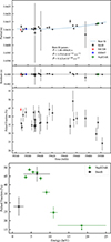 |
Fig. 2. Top: Values of the spin period measured in the single NICER, Swift, Insight-HXMT/LE, and NuSTAR observations in 2021 as a function of time. The blue dashed line indicates the best-fitting model (for more details see Sect. 3.3). The post-fit residuals are shown at the bottom. Middle: Evolution of the background-subtracted pulsed fraction of Sw J1555 as a function of time. Bottom: Background-subtracted pulsed fraction as a function of energy for the simultaneous Swift (black circle) and NuSTAR (green diamond) observations. The upper limit is reported at 3σ c.l. |
From the beginning of 2022 until the end of our campaign, the spin signal was only barely detected in the single Swift pointings. Therefore, we proceeded to analyse only the NICER data collected in 2022 July–August in an attempt to extract a phase-connected timing solution. Through epoch-folding techniques (Leahy et al. 1983), we first estimated a spin period P = 3.858(2) s in observation IDs 5202190101-5202190102 (which were merged for the timing analysis). Starting from this value and using a phase-fitting technique, we derived a phase-connected timing solution covering observations from Obs.ID 5202190101 (59781 MJD, 2022 July 21) to Obs.ID 5202190111 (59806 MJD, 2022 August 15). We did not include Obs.ID 5202190112 as the spin signal is barely detected in this dataset. For Obs. IDs 5202190106, 5202190110 and 5202190111, we only considered events in the energy range 2–7 keV, 2–6 keV and 1.8–7 keV, respectively, due to the high background level. We derived the following timing solution: P = 3.862065(1) s, Ṗ = 2.1(1) × 10−11 s s−1 at a reference epoch T0 = 59781.0 MJD (2022 July 21).
In all the observations where pulsations had been found, the pulse profile appeared single-peaked and quasi-sinusoidal. The middle panel of Figure 2 shows the variability of the pulsed fraction (here defined as the semi-amplitude of the best-fitting sinusoidal function to the profile divided by the source average net count rate) as a function of time, as derived using the NICER and Swift/XRT datasets in 2021. The pulsed fraction did not display significant variation over time, remaining consistently within the range ∼30–45% during our observations until October 15 (last observation where pulsations were significantly detected during 2021), when it dropped to ∼24%. No significant variability was also observed in the pulsed fraction of the NICER pulse profiles acquired in 2022. For the only epoch with a simultaneous NuSTAR observation, we detected pulsed emission up to ∼12 keV and derived a 3σ upper limit of ∼17% for the pulsed fraction in the 12–25 keV energy band. The pulsed fraction increased from ∼27% in the softer band (0.3–3 keV) to a maximum of ∼46% around 5–6 keV and then decreased with energy to ∼24%, as shown in the bottom panel of Figure 2. The same trend was already observed by Enoto et al. (2021) during the very early stage of the outburst.
We performed a phase-resolved spectral analysis using the NICER dataset acquired at the outburst onset. We divided the rotational phase cycle into ten intervals, each of width 0.1 in phase, and fitted an absorbed blackbody model to each phase-resolved spectrum. In the fits, NH was held fixed to the phase-averaged value, while all other parameters were allowed to vary. The overall fit quality was good, with χr2 = 0.98 for 177 dof. The results are shown in Figure 3. The modulation of the X-ray emission along the phase can be ascribed mainly to variations in the blackbody temperature, while the size of the emitting region seems to remain steady (fitting a constant term to the evolution of the blackbody radius as a function of phase gives RBB = 2.07 ± 0.05 km and χr2 = 0.66 for 9 d.o.f.). Tying up the blackbody radius across the phases resulted in an equally satisfactory fit, with χr2 = 1.02 for 186 d.o.f. On the other hand, linking the blackbody temperature across the phases led to a slightly worse fit, with χr2 = 1.20 for 186 d.o.f. We also performed phase-resolved spectral analysis on the 2022 NICER dataset. Due to the significantly lower count rate, we divided the rotational cycle into three equal phase bins to extract statistically meaningful spectra. In each bin, we fitted an absorbed blackbody model, keeping NH fixed to the phase-averaged value and allowing the blackbody temperature and radius to vary. All blackbody parameters in the three phase intervals were consistent with one another at the 2σ confidence level. This indicates no statistically significant phase-dependent variation in either temperature or emitting area in the 2022 data.
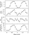 |
Fig. 3. From top to bottom: Background-subtracted pulse profile extracted from NICER data at the outburst peak in the 1.5–8 keV energy range, blackbody temperature, blackbody radius (assuming a distance of 10 kpc), 0.3–10 keV unabsorbed flux. All uncertainties are at 1σ c.l. For display purposes, the pulse profile has been shifted arbitrarily in phase, and two cycles are shown. |
3.4. Search for short X-ray bursts
We used the INTEGRAL archival data to look for short bursts from Sw J1555. However, during most pointings, Sw J1555 was at large off-axis angles in the partially coded field of view of IBIS, which reduced the sensitivity for burst detection. The burst search was performed by selecting events from the pixels that were illuminated by Sw J1555 for at least 50% of their area. We screened the light curves in the nominal 15–150 keV energy range binned at eight logarithmically spaced time resolutions between 0.01 to 1.28 s. Potential triggers were selected based on threshold levels corresponding to a chance occurrence of 10−3 in each ScW. After grouping together triggers at different timescales that belonged to the same event, we carried out an imaging analysis of each candidate. None of them could be confirmed as a point source event coming from the direction of Sw J1555. Therefore, we can conclude that no bursts from Sw J1555 were detected, with a typical upper limit of ∼2 × 10⁻⁸ erg cm−2 on the fluence in the 30–150 keV energy range (the exact value depends on the off-axis angle and background level in each ScW).
We also conducted a search for short bursts on the NICER, Swift, and NuSTAR light curves adopting different timing resolutions (2−4, 2−5, 2−6, 2−7, and 2−8 s), except for the Swift/XRT PC-mode event files that were binned at the available timing resolution (2.5073 s). We tagged as part of a burst every bin with a probability lower than 10−4(NNtrials)−1 of being a random fluctuation compared to the average count rate of the full observation, considering the total number of bins N and the timing resolutions Ntrials used in the search. We identified a total of 56 bursts, whose times of arrival are listed in Table B.1. Due to the low photon counting statistics, it was not possible to perform a meaningful spectral analysis of such events. During our monitoring campaign, Sw J1555 emitted a few short bursts that triggered the X-ray all-sky monitors (e.g. Swift/BAT, Enoto et al. 2021; GECAM, Zhang et al. 2022). We did not find any bursts in the Swift/XRT and NICER/XTI datasets that were simultaneous with the reported events.
3.5. Radio searches
The Parkes data were folded using the best X-ray ephemeris (Sect. 3.3) and searched over a period range spanning ±300 μs around the spin period at the epoch of the radio observations, and over a dispersion measure range from 0 to 1500 pc cm−3. The UWL data were also split into three sub-bands, 0.7–1 GHz, 1–2 GHz and 2–4 GHz, and folded independently. No periodic pulsations at the X-ray period were found in either dataset. The derived flux density upper limits for the three sub-bands are reported in Table A.2. We do not report values for the PDFB4 data since they were acquired over smaller bandwidths and thus all the resulting upper limits are significantly worse than those from the simultaneous data taken with the Medusa backend.
The single-pulse search for both backends was carried out via the SPANDAK7 (Gajjar et al. 2018) pipeline. The initial RFI purging is performed by SPANDAK through RFIFIND from the PRESTO8 package. The pipeline automates the search for bursts and single pulses using HEIMDALL (Barsdell et al. 2012), which performs a single pulse search by exploiting the matched filtering technique along a range of trial DMs. The search in DM of candidates run in the range from 0 to 2000 pc cm−3 and only candidates generated by HEIMDALL with S/N ≥ 8 and pulse width in the range 0.128–65.536 ms were selected. The search was carried out over both the full bandwidth (3328 MHz) by dividing that into sub-bands (1664 MHz, 832 MHz, and 416 MHz wide) and processing them individually (see e.g. Kumar et al. 2021). This was done to increase the sensitivity for single pulses with a spectral width smaller than the whole UWL bandwidth. We also considered additional sub-bands, shifted in frequency by a half sub-band for each of the mentioned explored cases. For data taken with the PDFB4 backend, it was not necessary to perform a sub-band search for candidates, given the smaller bandwidth. All candidates were also visually scrutinised to cross-check potential candidates found in each backend. No robust candidate possessing the characteristics of a fast radio burst was found with upper limits listed in Table A.2.
All the X-ray bursts on June 7 fell within the radio observation windows, and the same held true for all but the first burst on June 4 and for all but the last three bursts on June 5. Hence, the dedispersed radio time series were closely inspected (after a detailed manual cleaning) in a range of 30 s around the times of the occurrence of the X-ray bursts. No feature resembling a burst was observed down to S/N = 6, implying improved upper limits with respect to single pulse searches performed over the whole dataset (see Table A.2).
4. Discussion
We presented a comprehensive study of the first recorded outburst of the magnetar Swift J1555.2–5402, based on an extensive campaign of X-ray observations spanning nearly 29 months, and accompanied by deep radio searches. This source displays a suite of remarkable observational characteristics: a very slow flux decay in the first phases, followed by a fast dimming, a persistently high blackbody temperature with no variation over hundreds of days, and a spin-down evolution characterised by substantial variability. In the following, we place these findings in the broader context of magnetar phenomenology and theoretical modelling.
4.1. A prolonged bright plateau.
The persistent X-ray emission from Sw J1555 showed a remarkable evolution throughout our campaign. Over the first three weeks, the observed flux remained almost constant at ∼3.5 × 10⁻¹¹ erg cm−2 s−1; it exhibited a more rapid drop only in the final months, declining to ∼9 × 10⁻¹³ erg cm−2 s−1 by 2023 October. The overall light curve is well described by an exponential with e-folding timescale of ∼260 days. This prolonged plateau phase is unusual, but not unprecedented among magnetars. For example, SGR 1833−0832 and 1E 1048.1−5937 also displayed delayed flux decays following their 2010 and 2016 outbursts, respectively (Coti Zelati et al. 2018, and reference therein). However, the case of Sw J1555 appears even more extreme, as the flux remained above 10−11 erg cm−2 s−1 for more than 500 days, which is among the longest such intervals ever observed.
This evolution raises the question of whether the true outburst onset may have preceded the first detected burst on 2021 June 3. Although we cannot exclude this possibility, the high flux level observed after the activation, corresponding to a luminosity of (2–8)×1035 erg s−1 for a distance of 5–10 kpc, is comparable to the typical outburst peaks seen in magnetars. Moreover, this luminosity is close to the theoretical saturation limit imposed by neutrino cooling in the crust (as explored in early works Pons & Rea 2012 and recently reassessed in the cooling simulations by De Grandis et al. 2025) and to the maximum value predicted by twisted magnetosphere models (Beloborodov 2009). These findings suggest that the observed plateau likely reflects the actual early evolution of the outburst.
4.2. A constant temperature and an evolving emitting area.
A striking feature of the outburst from Sw J1555 is the constancy of its thermal spectral properties over a prolonged interval. The blackbody temperature remained approximately constant at kTBB ∼ 1.2 keV for over two years, while the emitting radius declined from ∼1.7 km to ∼0.3 km. This behaviour is consistent with the gradual contraction of a hot spot on the neutron star surface as the outburst decay and is similar to that seen in the outbursts of other high-temperature magnetars. In particular, both SGR J1830–0645 and Swift J1818.0−1607 exhibited similarly hot thermal components, with kT ≳ 1 keV, which remained stable for extended periods, during their latest outburst. In the case of SGR J1830–0645, Younes et al. (2022) reported a double blackbody spectrum (with components at ≃0.5 and 1.2 keV) that persisted for more than 220 days without significant evolution. For Swift J1818.0−1607, Hu et al. (2020) found that the thermal flux decayed by ≃60% over ≃100 days, with only a modest decrease in emitting radius, and the temperature remaining at around 1.1 keV as of late 2021 (Ibrahim et al. 2024). Another notable example is the 2017 outburst of CXOU J1647−4552, during which the inferred blackbody temperature attained a high constant value of ∼0.7 keV over ∼350 days (Borghese et al. 2019). Therefore, Sw J1555 appears to belong to a growing subset of magnetars that are able to maintain a small hot emitting region over long periods during outburst. This phenomenology points to sustained heating mechanisms, potentially linked to magnetospheric currents continuously depositing energy on localised regions of the neutron star surface. The nearly constant temperature, coupled with a shrinking area, is consistent with the gradual contraction of a heated spot rather than bulk cooling of the entire crust (see below).
Near the outburst peak, the flux modulation at the spin period is primarily driven by temperature variations, with little to no variation in the emitting area. This suggests that the hot region has a complex, non-uniform temperature distribution. Such temperature gradients could arise from localised heating by returning currents along twisted magnetic field bundles, possibly elongated or fan-shaped, and are expected in twisted magnetosphere models (Beloborodov 2009). An asymmetric thermal configuration can also appear in response to impulsive energy deposition within the star crust as the result of highly anisotropic heat transport to the surface in the presence of a complex magnetic field, as shown using 3D simulations (De Grandis et al. 2022). A similar behaviour has been observed in SGR J1830–0645 (Coti Zelati et al. 2021a; Younes et al. 2022), and XTE J1810−197 (Borghese et al. 2021), among others. In contrast, the 2022 NICER observations revealed no statistically significant phase-dependent variation in either temperature or radius. This likely reflects the lower photon statistics as well as a more compact and stable emitting region at later stages of the outburst.
4.3. Timing evolution and spin-down behaviour.
Our timing analysis provides a view of the rotational evolution of Sw J1555 over the first five months and a snapshot from the 2022 NICER observations. The period derivative Ṗ ∼ 3.6 × 10⁻¹¹ s s−1 measured during the first five months is slightly higher (∼15%) than that obtained during the first month by Enoto et al. (2021), suggesting a relatively stable spin-down torque during this phase. However, the data show evidence of timing noise, as testified by the presence of residuals in the fits with a polynomial.
Using the standard vacuum dipole formula, we estimate a surface dipolar magnetic field strength of Bdip ≃ 7.5 × 10¹⁴ G, a characteristic age τc ≃ 1.7 kyr, and a spin-down luminosity Ėrot ≃ 2.5 × 1034 erg s−1. These parameters place Sw J1555 among the strongly magnetised and relatively young members of the magnetar population.
The NICER timing campaign in mid-2022, almost a year after the outburst onset, yielded a lower spin-down rate, Ṗ ≃ 2.1 × 10⁻¹¹ s s−1. This likely indicates that the magnetosphere was relaxing back towards its pre-outburst configuration. Large changes in torque are commonly observed in magnetars during outbursts (e.g. Dib et al. 2012; Scholz et al. 2017; Archibald et al. 2020; Rajwade et al. 2022) and are generally attributed to the evolution of currents in twisted magnetospheres (see below for a discussion of such a scenario).
4.4. X-ray bursts and radio silence.
We identified 56 short X-ray bursts in our observations of Sw J1555, primarily during the early months of the outburst. This bursting activity is consistent with the behaviour of many magnetars during active phases.
No radio pulsations or bursts were detected in our three Parkes/Murriyang observations, either as periodic signals or as bursts coincident with X-ray bursts. This confirms the findings of Enoto et al. (2021), who also reported no radio emission from Sw J1555 using multiple telescopes. While a few active magnetars, including SGR 1935+2154 and Swift J1818.0−1607, have shown transient radio pulsations during or shortly after outbursts, not all magnetars are radio-loud. The absence of detectable radio emission from Sw J1555 may result from unfavourable viewing geometry, intrinsic emission properties, or absorption in the magnetosphere or local environment.
4.5. Implications for outburst mechanisms.
The outburst of Sw J1555 challenges the accepted paradigms in several respects. In the initial phases, the emission kept a high luminosity for an unusually long time span, with a nearly constant blackbody temperature. Subsequently, the temperature maintained a nearly constant value, with the flux and equivalent emission radii decaying following exponential profiles. The corresponding decay times are compatible with one being the double of the other, corresponding to a simple scenario in which the flux varies only due to the shrinking of the emission area. Figure 4 shows a comparison between the event at hand and the known outburst sample as described by Coti Zelati et al. (2018). Since the distance to this source is unknown, we normalised all the curves to the flux level at the outburst onset. Moreover, we highlight four other cases that display a similar morphology, namely, a rather stable initial phase followed by a substantial, rapid flux decay. Not only does Sw J1555 exhibit a very extended initial plateau, but the subsequent drop phase is much steeper than in other sources.
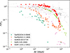 |
Fig. 4. Comparison between the long-term temporal evolution of the normalised flux for the major magnetar outbursts that occurred up to the end of 2016 with the outburst of Sw J1555 in red. The data are from the Magnetar Outburst Online Catalog (Coti Zelati et al. 2018). For SGR J1745−2900, we included the latest observations presented by Rea et al. 2020. The outbursts highlighted in colour are those showing a substantial and fast decay of the flux in the final phase, as observed for Sw J1555. |
Figure 5 shows a comparison between the data and a model of cooling of a crustal hotspot obtained with the methodology presented by De Grandis et al. (2025), which describes the evolution of the luminosity after an arbitrary amount of heat has been located in a small portion of the crust for a certain time. In order to reproduce the behaviour of the data (although performing a formal fit over the several model parameters is beyond the scope of this work), and in particular the long plateau phase, the time during which the heat is injected must be rather long, of the same order of the plateau itself (specifically, 400 days in the shown example). This implies either that the heat dissipation mechanism is long-lived, or that a sequence of multiple shorter heating episodes is active for an extended duration (see also Pons & Rea 2012). We note that, even though the model successfully describes the plateau phase, it cannot reproduce the features of the decay apart from the overall timescale, suggesting that several physical ingredients are still missing. Moreover, neutrino emission in the crust (Yakovlev et al. 2001) limits the maximum temperature that can be reached in the outermost layers (called the envelope). This was realised by Potekhin et al. (2015) and more recently reassessed by De Grandis et al. (2025), Kovlakas et al. (2025), who showed that considering a thin envelope (the appropriate assumption when treating short-term phenomena), this maximum temperature is higher than that sustainable in a thick envelope, reaching values of about 1 − 2 × 10⁷ K. This would match the observed value of 1.2 keV, corresponding to a surface temperature ∼1.7 × 10⁷ K accounting for the gravitational redshift on the surface of a standard neutron star with MNS = 1.4 M⊙ and RNS = 12 km.
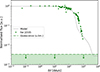 |
Fig. 5. Comparison between the flux evolution of Sw J1555 and a model of hotspot cooling modelled with the methodology by De Grandis et al. (2025), showing the evolution of a ∼1044 erg injection in a 3 km radius hotspot over a time of ∼400 days. |
An alternative (or complementary) explanation might involve prolonged magnetospheric currents in the spirit of twisted bundle models (Beloborodov 2009), whereby a slowly dissipating bundle of currents maintains surface heating over an extended period. If this twist is sustained or replenished, it could naturally account for the observed prolonged brightness along with the temperature gradients inferred from phase-resolved spectra, which point to a complex and possibly evolving magnetospheric configuration. In this framework, the initially twisted magnetic bundle inflates field lines and enhances the open-field region, thereby increasing the spin-down torque. As the twist dissipates, the radius of the hot region should shrink, and the torque should decrease monotonically. However, the variability seen in Sw J1555, and in other cases such as 1E 1048.1−5937 and Swift J1818.0−1607, suggests a more complex scenario, possibly involving the formation and dissipation of multiple rapidly evolving twisted regions. These could generate spatially and temporally variable currents, leading to torque fluctuations that are not strictly monotonic. Future modelling efforts should therefore explore whether scenarios involving multiple, evolving twists can simultaneously reproduce both the flux and torque evolution observed in Sw J1555.
Furthermore, outbursts have been modelled within the fallback disk paradigm (e.g. Ertan & Alpar 2003) by Çalışkan & Ertan (2012). They found that the luminosity of such events decays over the first ∼100 days as ∝t−n, with 0.5 ≲ n ≲ 1. This behaviour contrasts with both the remarkably flat evolution observed during the early phases of the event considered here and the subsequent steep decline (that would correspond to n ≳ 2). Therefore, the observed flux evolution of the outburst Sw J1555 is difficult to reconcile with this scenario.
5. Conclusions
We studied the long-term evolution of the X-ray properties of the magnetar Swift J1555.2–5402 during the first ∼29 months of its first (recorded) outburst, and analysed three radio observations carried out soon after the event onset without any successful detections.
The peculiarity of this outburst is its temporal evolution characterised by a long bright plateau of about 500 days followed by a sharp fast decline (see Fig. 4). Deep observations at late time are required to understand whether the source flux continued to decay below the quiescence upper limit or if it had already reached its (unknown) quiescent level. An additional puzzling trait is the blackbody temperature of ∼1.2 keV that remained constant during the entire duration of the monitoring campaign (∼29 months). These features represent a challenge for the outburst mechanisms proposed to date. While crustal cooling models are able to reproduce the plateau phase, they fail to model the fast decay in the final phase. On the other hand, detailed models concerning the un-twisting of magnetic field bundles in the magnetosphere are still missing.
Acknowledgments
We thank K. Gendreau for approving our NICER Target of Opportunity (ToO) requests and B. Cenko and the Swift duty scientists and science planners for making the Swift ToO observations possible. We thank the Insight-HXMT Science Operations Centre for promptly scheduling our ToO program. We thank the director of the Parkes/Murriyang Observatory for the prompt scheduling of our NAPA proposal. This research is based on observations with Swift (NASA/ASI/UKSA), NICER (NASA), NuSTAR (CalTech/NASA/JPL), Insight-HXMT (CNSA, CAS), INTEGRAL (ESA) and on data retrieved through the NASA/GSFC’s HEASARC archives. We used data collected at the Parkes/Murriyang radio telescope (proposal No. P1083), part of the Australia Telescope National Facility which is funded by the Australian Government for operation as a National Facility managed by CSIRO. We acknowledge the Wiradjuri people as the traditional owners of the Observatory site. A.B. acknowledges support through the European Space Agency (ESA) research fellowship programme. F.C.Z. is supported by a Ramón y Cajal fellowship (grant agreement RYC2021-030888-I). D.D.G. is supported by a Juan de la Cierva fellowship (grant agreement JDC2023-052264-I). F.C.Z., M.I., D.D.G. and N.R. are supported by the ERC Consolidator Grant “MAGNESIA” (No. 817661) and acknowledge funding from the Catalan grant SGR2021-01269 (PI: Graber/Rea), the Spanish grant ID2023-153099NA-I00 (PI: Coti Zelati), and by the program Unidad de Excelencia Maria de Maeztu CEX2020-001058-M. M.I. is also supported by the ERC Proof of Concept “DeepSpacePulse” (No. 101189496). G.L.I. and P.E. acknowledge financial support from the Italian MIUR through PRIN grant 2017LJ39LM. G.L.I. also acknowledges funding from ASI-INAF agreements I/037/12/0 and 2017-14-H.O. S.M. and D.P.P. acknowledge financial support through the INAF grants “Magnetars” and “Toward Neutron Stars Unification”. L.D. acknowledges funding from German Research Foundation (DFG), Projektnummer 549824807. M.B, S.M., M.P., and A.P. acknowledge resources from the research grant “iPeska” (PI: Possenti), funded under the INAF national call Prin-SKA/CTA approved with the Presidential Decree 70/2016. This work has been partially supported by the ASI-INAF program I/004/11/5.
References
- Archibald, R. F., Scholz, P., Kaspi, V. M., Tendulkar, S. P., & Beardmore, A. P. 2020, ApJ, 889, 160 [Google Scholar]
- Arnaud, K. A. 1996, in Astronomical Data Analysis Software and Systems V, eds. G. H. Jacoby, & J. Barnes (San Francisco: ASP), XSPEC: The First Ten Years, 101, 17 [NASA ADS] [Google Scholar]
- Barsdell, B. R., Bailes, M., Barnes, D. G., & Fluke, C. J. 2012, MNRAS, 422, 379 [CrossRef] [Google Scholar]
- Beloborodov, A. M. 2009, ApJ, 703, 1044 [NASA ADS] [CrossRef] [Google Scholar]
- Bernardini, M. G., Gropp, J. D., Kennea, J. A., et al. 2021, GCN, 30296, 1 [Google Scholar]
- Borghese, A., Rea, N., Turolla, R., et al. 2019, MNRAS, 484, 2931 [NASA ADS] [CrossRef] [Google Scholar]
- Borghese, A., Rea, N., Turolla, R., et al. 2021, MNRAS, 504, 5244 [NASA ADS] [CrossRef] [Google Scholar]
- Burrows, D. N., Hill, J. E., Nousek, J. A., et al. 2005, Space Sci. Rev., 120, 165 [Google Scholar]
- Çalışkan, Ş., & Ertan, Ü. 2012, ApJ, 758, 98 [CrossRef] [Google Scholar]
- Carrasco, F., Viganò, D., Palenzuela, C., & Pons, J. A. 2019, MNRAS, 484, L124 [Google Scholar]
- Collazzi, A. C., Kouveliotou, C., van der Horst, A. J., et al. 2015, ApJS, 218, 11 [Google Scholar]
- Cordes, J. M., & Lazio, T. J. W. 2002, arXiv e-prints [arXiv:astro-ph/0207156] [Google Scholar]
- Coti Zelati, F., Rea, N., Pons, J. A., Campana, S., & Esposito, P. 2018, MNRAS, 474, 961 [NASA ADS] [CrossRef] [Google Scholar]
- Coti Zelati, F., Borghese, A., Israel, G. L., et al. 2021a, ApJ, 907, L34 [NASA ADS] [CrossRef] [Google Scholar]
- Coti Zelati, F., Borghese, A., Rea, N., et al. 2021b, ATel, 14674, 1 [NASA ADS] [Google Scholar]
- De Grandis, D., Turolla, R., Taverna, R., et al. 2022, ApJ, 936, 99 [Google Scholar]
- De Grandis, D., Rea, N., Kovlakas, K., et al. 2025, A&A, 701, A229 [NASA ADS] [CrossRef] [EDP Sciences] [Google Scholar]
- Dehman, C., Viganò, D., Rea, N., et al. 2020, ApJ, 902, L32 [NASA ADS] [CrossRef] [Google Scholar]
- Dib, R., Kaspi, V. M., Scholz, P., & Gavriil, F. P. 2012, ApJ, 748, 3 [Google Scholar]
- Enoto, T., Ng, M., Hu, C.-P., et al. 2021, ApJ, 920, L4 [Google Scholar]
- Ertan, Ü., & Alpar, M. A. 2003, ApJ, 593, L93 [Google Scholar]
- Esposito, P., Rea, N., & Israel, G. L. 2021, in Magnetars: A Short Review and Some Sparse Considerations, eds. T. M. Belloni, M. Méndez, & C. Zhang (Berlin, Heidelberg: Springer), 97 [Google Scholar]
- Evans, P. A. 2021, ATel, 14675, 1 [Google Scholar]
- Gajjar, V., Siemion, A. P. V., Price, D. C., et al. 2018, ApJ, 863, 2 [NASA ADS] [CrossRef] [Google Scholar]
- Gendreau, K. C., Arzoumanian, Z., & Okajima, T. 2012, SPIE Conf. Ser., 8443, 844313 [Google Scholar]
- Goldwurm, A., David, P., Foschini, L., et al. 2003, A&A, 411, L223 [NASA ADS] [CrossRef] [EDP Sciences] [Google Scholar]
- Grefenstette, B., Bhargava, Y., Fuerst, F., et al. 2025, https://doi.org/10.5281/zenodo.14969199 [Google Scholar]
- Harrison, F. A., Craig, W. W., Christensen, F. E., et al. 2013, ApJ, 770, 103 [Google Scholar]
- Haslam, C. G. T., Salter, C. J., Stoffel, H., & Wilson, W. E. 1982, A&AS, 47, 1 [NASA ADS] [Google Scholar]
- Hobbs, G., Manchester, R. N., Dunning, A., et al. 2020, PASA, 37, e012 [NASA ADS] [CrossRef] [Google Scholar]
- Hu, C.-P., Begiçarslan, B., Güver, T., et al. 2020, ApJ, 902, 1 [NASA ADS] [CrossRef] [Google Scholar]
- Ibrahim, A. Y., Borghese, A., Coti Zelati, F., et al. 2024, ApJ, 965, 87 [Google Scholar]
- Kaastra, J. S., & Bleeker, J. A. M. 2016, A&A, 587, A151 [NASA ADS] [CrossRef] [EDP Sciences] [Google Scholar]
- Kaspi, V. M., & Beloborodov, A. M. 2017, ARA&A, 55, 261 [Google Scholar]
- Klingler, N. J., Page, K. L., Palmer, D. M., & Neil Gehrels Swift Observatory Team 2021, GCN, 30796, 1 [Google Scholar]
- Kovlakas, K., De Grandis, D., & Rea, N. 2025, A&A, 701, A267 [NASA ADS] [CrossRef] [EDP Sciences] [Google Scholar]
- Kumar, P., Shannon, R. M., Flynn, C., et al. 2021, MNRAS, 500, 2525 [Google Scholar]
- Leahy, D. A., Darbro, W., Elsner, R. F., et al. 1983, ApJ, 266, 160 [NASA ADS] [CrossRef] [Google Scholar]
- Mereghetti, S., Savchenko, V., Ferrigno, C., et al. 2020, ApJ, 898, L29 [Google Scholar]
- Ocker, S. K., & Cordes, J. M. 2024, Res. Notes AAS, 8, 17 [Google Scholar]
- Palmer, D. M., Evans, P. A., Kuin, N. P. M., Page, K. L., & Swift Team 2021, GCN, 30120, 1 [Google Scholar]
- Pons, J. A., & Rea, N. 2012, ApJ, 750, L6 [NASA ADS] [CrossRef] [Google Scholar]
- Potekhin, A. Y., Pons, J. A., & Page, D. 2015, Space Sci. Rev., 191, 239 [Google Scholar]
- Rajwade, K. M., Stappers, B. W., Lyne, A. G., et al. 2022, MNRAS, 512, 1687 [NASA ADS] [CrossRef] [Google Scholar]
- Rea, N., & De Grandis, D. 2025, arXiv e-prints [arXiv:2503.04442] [Google Scholar]
- Rea, N., Coti Zelati, F., Viganò, D., et al. 2020, ApJ, 894, 159 [CrossRef] [Google Scholar]
- Scholz, P., Camilo, F., Sarkissian, J., et al. 2017, ApJ, 841, 126 [Google Scholar]
- Tiengo, A., Vianello, G., Esposito, P., et al. 2010, ApJ, 710, 227 [Google Scholar]
- Turolla, R., Zane, S., & Watts, A. L. 2015, Rep. Progr. Phys., 78, 116901 [Google Scholar]
- Ubertini, P., Lebrun, F., Di Cocco, G., et al. 2003, A&A, 411, L131 [CrossRef] [EDP Sciences] [Google Scholar]
- Verner, D. A., Ferland, G. J., Korista, K. T., & Yakovlev, D. G. 1996, ApJ, 465, 487 [Google Scholar]
- Wilms, J., Allen, A., & McCray, R. 2000, ApJ, 542, 914 [Google Scholar]
- Yakovlev, D. G., Kaminker, A. D., Gnedin, O. Y., & Haensel, P. 2001, Phys. Rep., 354, 1 [NASA ADS] [CrossRef] [Google Scholar]
- Younes, G., Lander, S. K., Baring, M. G., et al. 2022, ApJ, 924, L27 [Google Scholar]
- Zhang, S.-N., Li, T., Lu, F., et al. 2020, Sci. China: Phys. Mech. Astron., 63, 249502 [Google Scholar]
- Zhang, Y. Q., Xiong, S. L., Xiao, S., et al. 2021, GCN, 30922, 1 [Google Scholar]
- Zhang, Y. Q., Xiao, S., Xiong, S. L., et al. 2022, GCN, 31397, 1 [Google Scholar]
The source had become too faint for the WT mode at these epochs for a meaningful spectral analysis.
INTEGRAL observations are divided into science windows, i.e. pointings with typical durations of ∼2–3 ks.
The null hypothesis probability (nhp) represents the probability that the deviations between the data and the model are due to chance alone. In general, a model can be rejected when the nhp is smaller than 0.05.
Upper limits (ULs) for the UWL are computed for the following sub-bands: 0.7-1.0 GHz, 1.0-2.0 GHz, 2.0-4.0 GHz. Both periodic emission and single pulse emission ULs are computed by exploiting the radiometer equation, assuming a S/N of 7 for pulsations and 6 for single pulses (see Sec. 3.5). We assumed a duty cycle of 10% for the pulsar emission and 1 ms for single pulses. System and Sky temperature, for each band, are evaluated from Hobbs et al. (2020) and Haslam et al. (1982), respectively. To compensate for eventual pulse smearing, due to propagation effects, we estimated the dispersion and scattering by using the NE2001 model (Cordes & Lazio 2002; Ocker & Cordes 2024).
Appendix A: Log of X-ray and radio observations
X-ray observation log with observed and unabsorbed fluxes.
Radio observation log with limits on periodic and single-pulse radio emission
Appendix B: Journal of the X-ray bursts
Table B.1 reports the times of arrival (in Barycentric Dynamical Time) and the fluence (in units of net counts) for all the X-ray bursts detected in the data presented in this work. The fluence values refer to the energy range 0.3–10 keV. For the bursts detected by Swift/XRT, the fluence values may not reflect the true intrinsic fluence, due to uncertainties related to the detector saturation limits.
The duration of each burst was estimated either by summing the time bins at the finer resolution showing enhanced emission or by setting it equal to the coarser time resolution at which the burst is detected. Therefore, it has to be considered as an approximate value. Except for burst #9 on 2021 June 5 (31.25 ms), burst #2 on June 21 (31.25 ms), and burst #1 on July 2 (125 ms), burst #1 on July 20 (39.06 ms), bursts #1 and #3 on 2022 June 19 (125 ms), all bursts have a duration of 62.5 ms according to our definition.
Log of X-ray Bursts.
All Tables
All Figures
|
Fig. 1. Temporal evolution of the blackbody temperature and radius, and of the observed and unabsorbed flux (0.3–10 keV) of Swift J1555.2–5402 over a time span of about 900 days since the epoch of the first Swift/BAT trigger (on 2021 June 3 at 09:45:46 UT; 59368.40678 MJD). The green dashed lines indicate the fit with an exponential function for the radius and observed flux. |
| In the text | |
|
Fig. 2. Top: Values of the spin period measured in the single NICER, Swift, Insight-HXMT/LE, and NuSTAR observations in 2021 as a function of time. The blue dashed line indicates the best-fitting model (for more details see Sect. 3.3). The post-fit residuals are shown at the bottom. Middle: Evolution of the background-subtracted pulsed fraction of Sw J1555 as a function of time. Bottom: Background-subtracted pulsed fraction as a function of energy for the simultaneous Swift (black circle) and NuSTAR (green diamond) observations. The upper limit is reported at 3σ c.l. |
| In the text | |
|
Fig. 3. From top to bottom: Background-subtracted pulse profile extracted from NICER data at the outburst peak in the 1.5–8 keV energy range, blackbody temperature, blackbody radius (assuming a distance of 10 kpc), 0.3–10 keV unabsorbed flux. All uncertainties are at 1σ c.l. For display purposes, the pulse profile has been shifted arbitrarily in phase, and two cycles are shown. |
| In the text | |
|
Fig. 4. Comparison between the long-term temporal evolution of the normalised flux for the major magnetar outbursts that occurred up to the end of 2016 with the outburst of Sw J1555 in red. The data are from the Magnetar Outburst Online Catalog (Coti Zelati et al. 2018). For SGR J1745−2900, we included the latest observations presented by Rea et al. 2020. The outbursts highlighted in colour are those showing a substantial and fast decay of the flux in the final phase, as observed for Sw J1555. |
| In the text | |
|
Fig. 5. Comparison between the flux evolution of Sw J1555 and a model of hotspot cooling modelled with the methodology by De Grandis et al. (2025), showing the evolution of a ∼1044 erg injection in a 3 km radius hotspot over a time of ∼400 days. |
| In the text | |
Current usage metrics show cumulative count of Article Views (full-text article views including HTML views, PDF and ePub downloads, according to the available data) and Abstracts Views on Vision4Press platform.
Data correspond to usage on the plateform after 2015. The current usage metrics is available 48-96 hours after online publication and is updated daily on week days.
Initial download of the metrics may take a while.